Chapter 3. Temporal-Difference Learning, Q-Learning, and n-Step Algorithms

Chapter 2 introduced two key concepts for solving Markov decision processes (MDPs). Monte Carlo (MC) techniques attempt to sample their way to an estimation of a value function. They can do this without explicit knowledge of the transition probabilities and can efficiently sample large state spaces. But they need to run for an entire episode before the agent can update the policy.

Conversely, dynamic programming (DP) methods bootstrap by updating the policy after a single time step. But DP algorithms must have complete knowledge of the transition probabilities and visit every possible state and action before they can find an optimal policy.

Note

A wide range of disciplines use the term bootstrapping to mean the entity can “lift itself up.” Businesses bootstrap by raising cash without any loans. Electronic transistor circuits use bootstrapping to raise the input impedance or raise the operating voltage. In statistics and RL, bootstrapping is a sampling method that uses individual observations to estimate the statistics of the population.

Temporal-difference (TD) learning is a combination of these two approaches. It learns directly from experience by sampling, but also bootstraps. This represents a breakthrough in capability that allows agents to learn optimal strategies in any environment. Prior to this point learning was so slow it made problems intractable or you needed a full model of the environment. Do not underestimate these methods; with the tools presented in this chapter you can design sophisticated automated systems. This chapter derives TD learning and uses it to define a variety of implementations.

Formulation of Temporal-Difference Learning

Recall that policies are dependent on predicting the state-value (or action-value) function. Once the agent has a prediction of the expected return, it then needs to pick the action that maximizes the reward.

Tip

Remember than an “expected” value is the arithmetic mean (the average) of a large number of observations of that value. For now, you can compute an average of all of the returns observed when you have visited that state in the past. And an online version of an average is an exponentially decaying moving average. But later in the book we will be using models to predict the expected return.

Equation 2-8 defined the state-value function as the expected return starting from a given state and you saw how to convert to an online algorithm in Equation 2-2. Equation 3-1 is an online realization of of the MC estimate of the state-value function. The key part is the exponentially weighted moving average estimate of the return, $G$. Over time, you update the state-value estimate to get closer to the true expected return and $\alpha$ controls the rate at which you update.

Equation 3-1. Online Monte Carlo state-value function

$$\begin{array}{cc}\hfill V_{\pi }\left(s\right)& \doteq {𝔼}_{\pi }\left[G\right|s]\hfill \\ & \leftarrow {𝔼}_{\pi }\left[V_{\pi }\left(s\right)+\alpha \left(G-V_{\pi }\left(s\right)\right)|s\right]\hfill \end{array}$$

Recall that $G$ is the total return from the entire trajectory. So the problem with Equation 3-1 is that you need to wait until the end of an episode before you have a value for $G$. So yes, it’s online in the sense that it updates one step at a time, but you still have to wait until the end of the episode.

The value estimate from “Value Iteration with Dynamic Programming” presented a slightly different interpretation of the state-value function. Instead of waiting until the end of an episode to observe the return, you can iteratively update the current state-value estimate using the discounted estimate from the next step. Equation 3-2 shows an online version of DP. It is online, by definition, because it looks one step ahead all the time. Note that this equation starts from the same definition of the state-value function as the MC version.

Equation 3-2. Online dynamic programming state-value function

$$\begin{array}{cc}\hfill V_{\pi }\left(s\right)& \doteq {𝔼}_{\pi }\left[G\right|s]\hfill \\ & \leftarrow \underset{a}{max}\sum _{s^{\text{'}},r}p(s^{\text{'}},r\mid s,a)\left[r+\gamma V\left(s^{\text{'}}\right)\right]\hfill \end{array}$$

You already know that the issue here is that you don’t know the transition probabilities. But notice in the final line of Equation 3-2 that the DP version is using an interesting definition for $G$, $r+\gamma V\left(s^{\text{'}}\right)$. This is saying the return is equal to the current reward plus the discounted prediction of the next state. In other words, the return is the current reward, plus the estimate of all future rewards. Is it possible to use this definition of $G$ in the Monte Carlo algorithm so you don’t have to wait until the end of an episode? Yes! Look at Equation 3-3.

Equation 3-3. Temporal-difference state-value function

$$V_{\pi }\left(s\right)\doteq {𝔼}_{\pi }\left[V_{\pi }\left(s\right)+\alpha \left(r+\gamma V_{\pi }\left(s^{\text{'}}\right)-V_{\pi }\left(s\right)\right)|s\right]$$

Equation 3-3 is the TD estimate of the expected return. It combines the benefits of bootstrapping with the sampling efficiency of the MC rolling average. Note that you could reformulate this equation to estimate the action-value function as well.

Finally, I can convert this to an online algorithm, which assumes that an exponentially weighted average is a suitable estimate for the expectation operator, and results in the online TD state-value estimate in Equation 3-4.

Equation 3-4. Online temporal-difference state-value function

$$V_{\pi }\left(s\right)\leftarrow V_{\pi }\left(s\right)+\alpha \left(r+\gamma V_{\pi }\left(s^{\text{'}}\right)-V_{\pi }\left(s\right)\right)$$

Take a moment to let these equations sink in; try to interpret the equations in your own words. They say that you can learn an optimal policy, according to an arbitrary definition of reward, by dancing around an environment and iteratively updating the state-value function according to Equation 3-3. The updates to the state-value function, and therefore the policy, are immediate, which means your next action should be better than the previous.

Q-Learning

In 1989, an implementation of TD learning called Q-learning made it easier for mathematicians to prove convergence. This algorithm is credited with kick-starting the excitement in RL. You can reformulate Equation 3-3 to provide the action-value function (Equation 2-9). In addition, Equation 3-5 implements a simple policy by intentionally choosing the best action for a given state (in the same way as in Equation 2-10).

Equation 3-5. Q-learning online update rule to estimate the expected return

$$Q(s,a)\leftarrow Q(s,a)+\alpha \left(r+\gamma \underset{a_s\in 𝒜\left(s\right)}{argmax}Q(s^{\text{'}},a_s)-Q(s,a)\right)]$$

Recall that $Q(s,a)$ is the action-value function, the one from Equation 2-9 that tells you the expected return of each action. Equation 3-5 is implemented as an online update rule, which means you should iterate to refine the estimate of $Q(s,a)$ by overwriting the previous estimate. Think of everything to the right of the $\alpha$ as a delta, a measure of how wrong the estimate is compared to what actually happened. And the TD one-step look-ahead implemented in the delta allows the algorithm to project one step forward. This allows the agent to ask, “Which is the best action?”

This is the most important improvement. Previous attempts estimated the expected return for each state using only knowledge of that state. Equation 3-5 allows the agent to look ahead to see which future trajectories are optimal. This is called a rollout. The agent rolls out the states and actions in the trajectory (up to a maximum of the end of an episode, like for MC methods). The agent can create policies that are not only locally optimal, but optimal in the future as well. The agent can create policies that can predict the future.

This implementation of the action-value function is particularly special, though, for one simple addition. The argmax from Equation 3-5 is telling the algorithm to scan over all possible actions for that state, and pick the one with the best expected return.

This active direction of the agent is called Q-learning and is implemented in Algorithm 3-1.

Algorithm 3-1. Q-learning (off-policy TD)

$$\begin{array}{cc}\hfill \text{1:}& 𝐢𝐧𝐩𝐮𝐭\text{:}\text{a}\text{policy}\text{that}\text{uses}\text{the}\text{action-value}\text{function,}\pi \left(a\mid s,Q(s,a)\right)\hfill \\ \hfill \text{2:}& \text{Initialize}Q(s,a)\leftarrow 0,\text{for}\text{all}s\in 𝒮,a\in 𝒜\left(s\right)\hfill \\ \hfill \text{3:}& 𝐥𝐨𝐨𝐩\text{:}\text{for}\text{each}\text{episode}\hfill \\ \hfill \text{4:}& \text{Initialize}\text{environment}\text{to}\text{provide}s\hfill \\ \hfill \text{5:}& 𝐝𝐨\text{:}\hfill \\ \hfill \text{6:}& \text{Choose}a\text{from}s\text{using}\pi \text{,}\text{breaking}\text{ties}\text{randomly}\hfill \\ \hfill \text{7:}& \text{Take}\text{action,}a\text{,}\text{and}\text{observe}r,s\text{'}\hfill \\ \hfill \text{8:}& Q(s,a)\leftarrow Q(s,a)+\alpha \left[r+\gamma \underset{a_s\in 𝒜\left(s\right)}{argmax}Q(s^{\text{'}},a_s)-Q(s,a)\right]\hfill \\ \hfill \text{9:}& s\leftarrow s\text{'}\hfill \\ \hfill \text{10:}& 𝐰𝐡𝐢𝐥𝐞s\text{is}\text{not}\text{terminal}\hfill \end{array}$$

Algorithm 3-1 shows an implementation of Q-learning. You should recognize most of this algorithm as it is closely related to Algorithm 2-3 and Algorithm 2-4. As before, step (1) begins by passing in a policy that is used to decide the probability of which action to take (which might implement $ϵ$-greedy exploration from Algorithm 2-1, for example). Step (2) initializes an array to store all the action-value estimates. This can be efficiently implemented with a map that automatically defaults to a set value.

Step (3) iterates over all episodes and step (5) iterates over each step in an episode. Step (4) initializes the starting state. Environments typically provide a function to “reset” the agent to a default state.

Step (6) uses the external policy function to decide which action to take. The chosen action is that with the highest probability. I have made this more explicit than it is typically presented in the literature because I want to make it clear that there is never a single optimal action. Instead, a range of actions have some probability of being optimal. Q-learning picks the action with the highest probability, which is often derived from the largest value of $Q(s,a)$. And you can implement $ϵ$-greedy by setting all actions to the same probability, for some proportion of the time, for example.

Step (7) uses the chosen action in the environment and observes the reward and next state. Step (8) updates the current action-value estimate for the given state and action based upon the new behavior observed in the environment. Remember that the expected return is calculated as the sum of the current reward and the expected value of the next state. So the delta is this minus the expected value of the current state. Step (8) also exponentially decays the delta using the $\alpha$ parameter, which helps to average over noisy updates.

Step (9) sets the next state and finally step (10) repeats this process until the environment signals that the state is terminal. With enough episodes [step (3)], the action-value estimate approaches the correct expected return.

Look at the end of Algorithm 3-1, in step (8). Notice the TD error term on the right. $\underset{a_s\in 𝒜\left(s\right)}{argmax}Q(s^{\text{'}},a_s)$ looks over all possible actions for that next state and chooses the one with the highest expected return. This has nothing to do with the action chosen in step (6). Instead, the agent is planning a route using future actions.

This is the first practical example of an off-policy agent. The algorithm is off-policy because the update only affects the current policy. It does not use the update to direct the agent. The agent still has to derive the action from the current policy. This is a subtle, but crucial improvement that has only recently been exploited. You can find more examples of off-policy algorithms later in the book.

Another thing to note is the use of the array in step (2). It stores the expected value estimate for each state-action pair in a table, so this is often called a tabular method. This distinction is important because it means you cannot use Algorithm 3-1 when you have continuous states or actions, which would lead to an array of infinite length. You will see methods that can natively handle continuous states in Chapter 4 or actions in Chapter 5. You can learn how to map continuous to discrete values in Chapter 9.

SARSA

SARSA was developed shortly after Q-learning to provide a more general solution to TD learning. The main difference from Q-learning is the lack of $argmax$ in the delta. Instead it calculates the expected return by averaging over all runs (in an online manner).

You can observe from Equation 3-6 that the name of this particular implementation of TD learning comes from the state, action, and reward requirements to calculate the action-value function. The algorithm for SARSA is shown in Algorithm 3-2.

Equation 3-6. SARSA online estimate of the action-value function

$$Q(s,a)\leftarrow Q(s,a)+\alpha \left(r+\gamma Q(s^{\text{'}},a^{\text{'}})-Q(s,a)\right)$$

Both Algorithm 3-2 and Algorithm 3-1 have hyperparameters. The first is $\gamma$, the factor that discounts the expected return, introduced in Equation 2-7. The second is the action-value learning rate, $\alpha$, which should be between 0 and 1. High values learn faster but perform less averaging.

Algorithm 3-2. SARSA (on-policy TD)

$$\begin{array}{cc}\hfill \text{1:}& 𝐢𝐧𝐩𝐮𝐭\text{:}\text{a}\text{policy}\text{that}\text{uses}\text{the}\text{action-value}\text{function,}\pi \left(a\mid s,Q(s,a)\right)\hfill \\ \hfill \text{2:}& \text{Initialize}Q(s,a)\leftarrow 0,\text{for}\text{all}s\in 𝒮,a\in 𝒜\left(s\right)\hfill \\ \hfill \text{3:}& 𝐥𝐨𝐨𝐩\text{:}\text{for}\text{each}\text{episode}\hfill \\ \hfill \text{4:}& \text{Initialize}\text{environment}\text{to}\text{provide}s\hfill \\ \hfill \text{5:}& 𝐝𝐨\text{:}\hfill \\ \hfill \text{6:}& \text{Choose}a\text{from}s\text{using}\pi \text{,}\text{breaking}\text{ties}\text{randomly}\hfill \\ \hfill \text{7:}& \text{Take}\text{action,}a\text{,}\text{and}\text{observe}r,s\text{'}\hfill \\ \hfill \text{8:}& \text{Choose}a\text{'}\text{from}s\text{'}\text{using}\pi \text{,}\text{breaking}\text{ties}\text{randomly}\hfill \\ \hfill \text{9:}& Q(s,a)\leftarrow Q(s,a)+\alpha \left[r+\gamma Q(s^{\text{'}},a\text{'})-Q(s,a)\right]\hfill \\ \hfill \text{10:}& s\leftarrow s\text{'},a\leftarrow a\text{'}\hfill \\ \hfill \text{11:}& 𝐰𝐡𝐢𝐥𝐞s\text{is}\text{not}\text{terminal}\hfill \end{array}$$

Algorithm 3-2 is almost the same as Algorithm 3-1, so I won’t repeat the explanation in full. One difference is that the algorithm chooses the next action, $a\text{'}$, in step (8), before it updates the action-value function in step (9). $a\text{'}$ updates the policy and directs the agent on the next step, which makes this an on-policy algorithm.

The differences between on-policy and off-policy algorithms magnify when applying function approximation, which I use in Chapter 4. But do these subtleties actually make any difference? Let me test these algorithms to show you what happens.

Q-Learning Versus SARSA

One classic environment in the RL literature is the Gridworld, a two-dimensional grid of squares. You can place various obstacles in a square. In the first example I place a deep hole along one edge of the grid. This is simulating a cliff. The goal is to train an agent to navigate around the cliff from the starting point to the goal state.

I design the rewards to promote a shortest path to the goal. Each step has a reward of −1, falling off the cliff has a reward of −100, and the goal state has a reward of 0. The cliff and the goal state are terminal states (this is where the episode ends). You can see a visualization of this environment in Figure 3-1.

To demonstrate the differences I have implemented Q-learning and SARSA on the accompanying website. There you will also find an up-to-date list of current RL frameworks. And I talk more about the practicalities of implementing RL in Chapter 9.

Figure 3-1. A depiction of the grid environment with a cliff along one side.¹

If I train these agents on the environment described in Figure 3-1, I can record the episode rewards for each time step. Because of the random exploration of the agent, I need to repeat the experiment many times to average out the noise. You can see the results in Figure 3-2, in which the plots show the average sum of rewards over 100 parallel experiments.

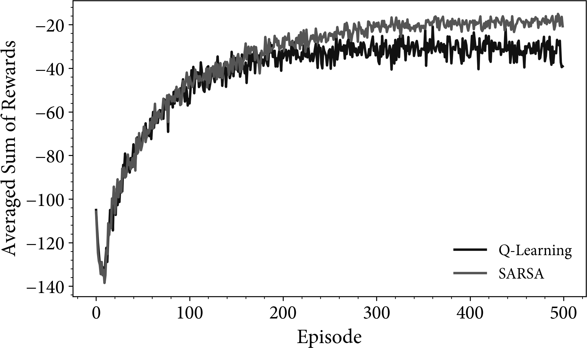
Figure 3-2. A comparison of Q-learning against SARSA for a simple grid problem. The agents were trained upon the environment in Figure 3-1. I used $\gamma \doteq 1.0$, $ϵ\doteq 0.1$, and $\alpha \doteq 0.5$. The rewards for each episode were captured and averaged over 100 trials.

Tip

Recall that an episode is one full experiment, from the starting point to a terminal node, which in this case is falling off the cliff or reaching the end. The x-axis in Figure 3-2 is the episode number. 500 episodes mean 500 terminal events.

Figure 3-2 has two interesting regions. The first is the dip at the start of the learning. The performance of the first episode was better than the fifth. In other words, a random agent has better performance than one trained for five episodes. The reason for this is the reward structure. I specified a reward of −100 for falling off the cliff. Using a completely random agent, with the start so close to the cliff, you should expect the agent to fall off pretty much immediately. This accounts for the near −100 reward at the start. However, after a few trials, the agent has learned that falling off the cliff is not particularly enjoyable, so it attempts to steer away. Moving away results in a −1 reward per step, and because the cliff is quite long and the agent does not have much experience of reaching the goal state yet, it wastes steps then falls off the cliff anyway—a tough life. The sum of the negative reward due to the wasted steps and the eventual cliff dive results in a lower reward than when the agent started (approximately −125).

This is an interesting result. Sometimes you need to accept a lower reward in the short term to find a better reward in the long run. This is an extension of the exploitation versus exploration problem.

The second interesting result is that the SARSA result tends to have a greater reward and be less noisy than Q-learning. The reason for this can be best described by the resulting policies.

Figure 3-3 shows example policies for Q-learning and SARSA. Note that the specific policy may change between trials due to the random exploration. The SARSA agent tends to prefer the “safe” path, far away from the cliff. This is because occasionally, the $ϵ$-greedy action will randomly kick the agent over the cliff. Recall that SARSA is calculating the average expected return. Hence, on average, the expected return is better far away from the cliff because the chances of receiving three random kicks toward the cliff are slim.

However, the Q-learning algorithm does not predict the expected return. It predicts the best possible return from that state. And the best one, when there is no random kick, is straight along the cliff edge. A risky but, according to the definition of the reward, optimal policy.

This also explains the difference in variance. Because Q-learning is metaphorically on a knife edge, it sometimes falls off. This causes a massive but sporadic loss. The SARSA policy is far away from the cliff edge and rarely falls, so the rewards are more stable.

Figure 3-3. The policies derived by Q-learning and SARSA agents. Q-learning tends to prefer the optimal route. SARSA prefers the safe route.

Case Study: Automatically Scaling Application Containers to Reduce Cost

Software containers are changing the way that distributed applications are deployed and orchestrated in the cloud. Their primary benefit is the encapsulation of all run-time dependencies and the atomicity of the deployable unit. This means that applications can be dynamically scaled both horizontally, through duplication, and vertically, by increasing the allocated resources. Traditional scaling strategies rely on fixed, threshold-based heuristics like utilized CPU or memory usage and are likely to be suboptimal. Using RL to provide a scaling policy can reduce cost and improve performance.

Rossi, Nardelli, and Cardellini proposed an experiment to use both Q-learning and a model-based approach to provide optimal policies for scaling both vertically and horizontally.2 They then implemented these algorithms in a live Docker Swarm environment.

Rossi et al. begin by using a generic black-box container that performs an arbitrary task. The agent interacts with the application through the confines of a Markov decision process.

The state is defined as the number of containers, the CPU utilization, and the CPU allocation to each container. They quantize the continuous variables into a fixed number of bins.

The action is defined as a change to the horizontal or vertical scale of the application. They can add or remove a replica, add or remove allocated CPUs, or both. They perform two experiments: the first simplifies the action space to only allow a single vertical or horizontal change, while the second allows both.

The reward is quite a complex function to balance the number of deployment changes, the latency, and utilization. These metrics have arbitrary weightings to allow the user to specify what is important to their application.

Although Rossi et al. initially used a simulator to develop their approach, they thankfully tested their algorithm in real life using Docker Swarm. They implemented a controller to monitor, analyze, plan, and execute changes to the application. Then they simulated user requests using a varying demand pattern to stress the application and train the algorithms to maximize the reward.

There are several interesting results from this experiment. First, they found that the algorithms were quicker to learn when they used a smaller action space in the experiment where the agent had to choose to scale vertically or horizontally, not both. This is a common result; smaller state and action spaces mean that the agent has to explore less and can find an optimal policy faster. During the simple experiment both the Q-learning and model-based approaches performed similarly. With the more complex action space, the model-based approach learned quicker and the results were much better.

The second interesting result is that using a model, bespoke to this challenge, improves learning and final performance. Their model-based approach incorporates transition probabilities into the value approximation, much like you did in “Inventory Control”, so the algorithm has prior knowledge of the effect of an action. However, their model implicitly biases the results toward that model. This is shown in the results when the model-based approach prefers to scale vertically more than horizontally. In most modern orchestrators it is much easier to scale horizontally, so this would be a detriment. The moral of this is that yes, model-based approaches introduce prior knowledge and significantly speed up learning, but you have to be sure that the model represents the true dynamics of the system and there is no implicit bias toward a certain policy.

The net result in either case is a significant improvement over static, threshold-based policies. Both algorithms improved utilization by an order of magnitude (which should translate into costs savings of an order of magnitude) while maintaining similar levels of latency.

You could improve this work in a number of ways. I would love to see this example implemented on Kubernetes and I would also like to see rewards using the real cost of the resources being used, rather than some measure of utilization. I would improve the state and action representations, too: using function approximation would remove the need to discretize the state, and a continuous action could choose better vertical scaling parameters. I would also be tempted to split the problem as well, because scaling vertically and horizontally has very different costs; in Kubernetes at least, it is much easier to scale horizontally.

Industrial Example: Real-Time Bidding in Advertising

Contrary to sponsored advertising, where advertisers set fixed bids, in real-time bidding (RTB) you can set a bid for every individual impression. When a user visits a website that supports ads, this triggers an auction where advertisers bid for an impression. Advertisers must submit bids within a period of time, where 100 ms is a common limit.

The advertising platform provides contextual and behavioral information to the advertiser for evaluation. The advertiser uses an automated algorithm to decide how much to bid based upon the context. In the long term, the platform’s products must deliver a satisfying experience to maintain the advertising revenue stream. But advertisers want to maximize some key performance indicator (KPI)—for example, the number of impressions or click-through rate (CTR)—for the least cost.

RTB presents a clear action (the bid), state (the information provided by the platform), and agent (the bidding algorithm). Both platforms and advertisers can use RL to optimize for their definition of reward. As you can imagine, the raw bid-level impression data is valuable. But in 2013 a Chinese marketing company called iPinYou released a dataset hoping that researchers could improve the state of the art in bidding algorithms.3

Defining the MDP

I will show how simple RL algorithms, like Q-learning and SARSA, are able to provide a solution to the RTB problem. The major limitation of these algorithms is that they need a simple state space. Large or continuous states are not well suited because agents need many samples to form a reasonable estimate of the expected value (according to the law of large numbers). Continuous states cause further problems because of the discrete sampling. For tabular algorithms, you have to simplify and constrain the state to make it tractable.

I propose to create an RTB algorithm that maximizes the number of impressions for a given budget. I split the data into batches and each batch has a budget. The state consists of the average bid that the agent can make given the number of auctions remaining. For example, if the budget is 100 and the batch size is 10, then at the first auction the state is $100/10=10$. The purpose of this feature is to inform the agent that I want to spread the bids throughout the batch. I don’t want the agent to spend the budget all at once. The agent will receive a reward of one if they win the auction and zero otherwise. To further reduce the number of states I round and truncate the real number to an integer. Later you will see examples of agents that are able to fit a function to the state to allow it to capture far more complex data.

This highlights an important lesson. The formulation of the MDP is arbitrary. You can imagine many different pieces of information to include in the state or create another reward. You have to design the MDP according to the problem you are trying to solve, within the constraints of the algorithm. Industrial data scientists rarely alter the implementation details of a machine learning algorithm; they are off-the-shelf. RL practitioners spend most of the time improving the representation of the state (typically called feature engineering) and refining the definition of reward. Industrial ML is similar, where a data scientist spends the majority of their time improving data or reformulating problems.

Results of the Real-Time Bidding Environments

I created two new environments. The first is a static RTB environment I built for testing. Each episode is a batch of 100 auctions and I fix the budget at 10,000. If the agent bids a value of greater than or equal to 100, it will win the auction. Hence, the optimal policy for this environment is to bid 100 at each auction to receive a reward of 100. The agent can increase or decrease the current bid by 50%, 10% or 0%. You can see the results in Figure 3-4.

This isn’t very realistic but demonstrates that the algorithm implementations are working as expected. Despite learning the optimal policy, this plot does not reach a reward of 100 because of the high $ϵ$. That is, while obtaining these rewards the agent is still taking random (often incorrect) actions. There is also a subtle difference between SARSA and Q-learning, because SARSA prefers the safer path of slightly overbidding, which means it runs out of budget quicker than Q-learning; this is the same as what you saw in “Q-Learning Versus SARSA”.

The second environment uses real bidding data. If you follow the instructions from the make-ipinyou-data repository, you will have directories that represent advertisers. Inside, these files contain the predicted CTR, whether a user actually clicked the ad, and the price of the winning bid. The batch size and the agent’s actions are the same as before. The main difference is that the cost of winning the auction is now variable. The goal, as before, is to train an agent to win the most impressions for the given budget. I also make the situation more difficult by setting the agent’s initial bid too low. The agent will have to learn to increase its bid. You can see the results in Figure 3-5.

Figure 3-4. The average reward obtained by SARSA, Q-learning, and random agents in a simple, static, real-time bidding environment.

Figure 3-5. The average reward obtained by SARSA, Q-learning, and random agents in an environment based upon real data. The agent obtains a greater reward as episodes pass. The reason is that the agent has learned, through random exploration, that increasing the bid leads to greater rewards. Allowing the agent to continue learning is likely to increase the reward further.

Further Improvements

The previous example constrained the RTB problem because I needed to simplify the state space. Tabular methods, such as Q-learning and SARSA, struggle when the state space is large; an agent would have to sample a huge, possibly infinite, number of states. Later in the book you will see methods that build a model of the state space, rather than a lookup table.

Another concern is the choice of reward. I chose to use the impression count because this led to learning on each time step and therefore speeds up learning. It might be beneficial to instead use user clicks as a reward signal, since advertisers are often only interested if a user actually clicks their ad.

I also limited the amount of data used in training to allow the learning to complete in a matter of seconds; otherwise it takes hours to run. In an industrial setting you should use as much data as you can to help the agent generalize to new examples.

The initial bid setting is inappropriate because I am forcing the agent to learn from an extreme. I did this to show that the agent can learn to cope with new situations, like when a new, well-funded advertiser attempts to capture the market by outbidding you. A more realistic scenario might be to not reset the initial bid and carry it through from the previous episode.

To improve the resiliency and stability of the agent you should always apply constraints. For example, you could use error clipping to prevent outliers from shifting the expected return estimates too far in one go (see “PPO’s clipped objective” for an example of an algorithm that does this).

One paper takes batching one step further by merging a set of auctions into a single aggregate auction. The agent sets the bid level at the start and keeps it the same throughout the batch. The benefit is that this reduces the underlying volatility in the data through averaging.

The data exhibits temporal differences, too. At 3 A.M. fewer auctions take place and fewer advertisers are available compared to at 3 P.M. These two time periods require fundamentally different agents. Including the user’s time in the agent state allows the agent to learn time-dependent policies.

The actions used within this environment were discrete alterations to the bid. This reduces the size of the state-action lookup table. Allowing the agent to set the value of the alteration is preferable. It is even possible to allow the agent to set the bid directly using algorithms that can output a continuously variable action.

That was a long list of improvements and I’m sure you can think of a lot more. But let me be clear that choosing the RL algorithm is often one of the easiest steps. This example demonstrates that in industry you will spend most of your time formulating an appropriate MDP or improving the features represented in the state.

Extensions to Q-Learning

Researchers can improve upon TD algorithms in a wide variety of ways. This section investigates some of the most important improvements specifically related to SARSA and Q-learning. Some improvements are better left until later chapters.

Double Q-Learning

Equation 3-5 updates $Q(s,a)$ using a notion of the best action, which in this case is the action that produces the highest expected reward. The problem with this is that the current maximum may be a statistical anomaly. Consider the case where the agent has just started learning. The first time the agent receives a positive reward, it will update the action-value estimate. Subsequent episodes will repeatedly choose the same set of actions. This could create a loop where the agent keeps making sub-optimal decisions, because of that initial bad update.

One way to solve this problem is by using two action-value functions, in other words, two lookup tables.4 The agent then uses one to update the other and vice versa. This produces an unbiased estimate of $Q(s,a)$, because it is not feeding back into itself. Typically the choice of which combination to update, for example updating $Q_1$ with the action-value estimate of $Q_2$, is random.

Delayed Q-Learning

In probably the best named computational theory of all time, probably approximately correct (PAC) learning states that for a given hypothesis, you need a specific number of samples to solve the problem within an acceptable error bound. In 2006 mathematicians developed a Q-learning-based algorithm based on this principle called delayed Q-learning.5

Rather than update the action-value function every time the agent visits that state-action pair, it buffers the rewards. Once the agent has visited a certain number of times, it then updates the main action-value function in one big hurrah.

The idea, due to the law of large numbers again, is that one estimate of the expected return could be noisy. Therefore, you should not update the main action-value table with potentially erroneous values, because the agent uses this to direct future agents. You should wait for a while and update only when there is a representative sample.

The downside of this approach is that it leads to a certain amount of delay before you begin to get good results. But once you do, learning is very quick, because the agent is not blighted by noise.

In a sense, this is just a way to prolong the exploration period. You get a similar effect if you anneal the $ϵ$ in $ϵ$-greedy or use UCB (see “Improving the $ϵ$-greedy Algorithm”). A similar implementation called directed delayed Q-learning also integrates an exploration bonus for action-state pairs that have not been well sampled.⁶

Comparing Standard, Double, and Delayed Q-learning

Figure 3-6 compares the performance of standard, double, and delayed Q-learning on the grid environment. The double Q-learning implementation results in a better policy than standard Q-learning as shown in the higher average result (it will keep on improving if you give it more time; compare with Figure 3-2). For the delayed Q-learning implementation, the apparent discontinuities are worrying with respect to robustness, but the end result is very impressive. This is because the aggregation of many updates provides a more robust estimate of the action-value function. The flat region at the top is because delayed Q-learning intentionally stops learning after a certain number of updates.

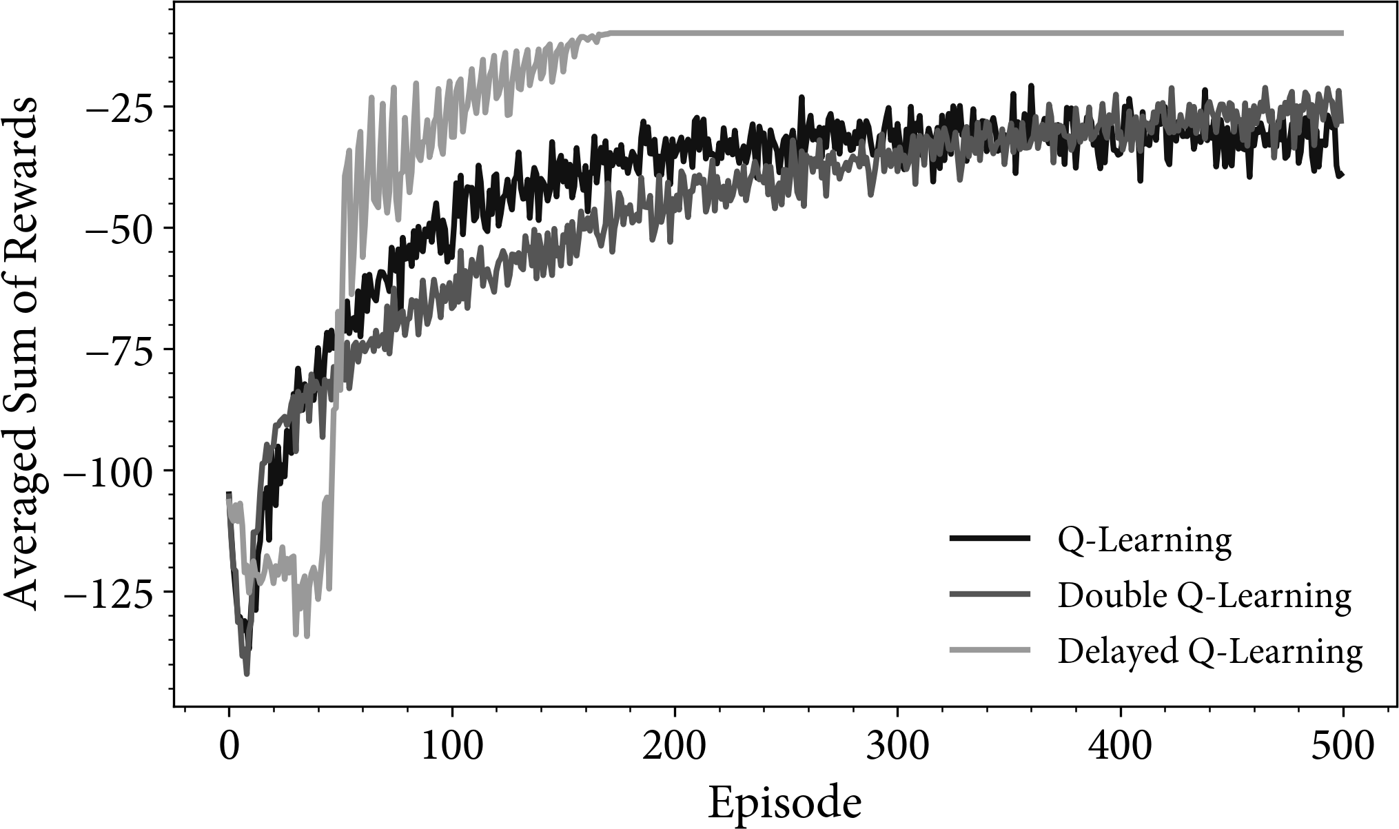
Figure 3-6. A comparison between the averaged rewards of standard, double, and delayed Q-learning on the grid environment.

Opposition Learning

In an interesting addition, Tizhoosh attempted to improve learning performance by intentionally sampling the opposite of whatever the policy chooses.7 Known as Opposition-Based RL, the Q-learning inspired implementation intentionally samples and updates the opposite action as well as the action chosen by the current policy. The gist of this idea is that an opposite action can reveal a revolutionary or counter-factual move, an action that the policy would never have recommended.

If a natural opposite exists then this is likely to yield faster learning in the early stages, because it prevents the worst-case scenario. However, if none exists then you might as well sample randomly, which amounts to a normal update and a random one. If that is acceptable, I could cheat and sample all actions.

The main issue with this is that in many environments you can’t test multiple actions at the same time. For example, imagine you tried to use this algorithm on a robot. It would have to take the opposite (or random) action, move back, then take the policy action. The act of moving back may be imprecise and introduce errors. This also doesn’t map well to continuous domains. A better approach is to prefer using multiple agents or separate critical policies to generate counteractions.

n-Step Algorithms

This chapter has considered a one-step lookahead. But why stop there? Why not have a two-step lookahead? Or more? That is precisely what $n$-step algorithms are all about. They provide a generalization of unrolling the expected value estimate to any number of steps. This is beneficial because it bridges the gap between dynamic programming and Monte Carlo.

For some applications it makes sense to look several steps ahead before making a choice. In the grid example, if the agent can see that the current trajectory is leading the agent to fall off the cliff, the agent can take avoiding action now, before it becomes too late. In a sense, the agent is looking further into the future.

The essence of the idea is to extend one of the TD implementations, Equation 3-3 for example, to iterate over any number of future states. Recall that the lookahead functionality came from DP (Equation 3-3), which combined the current reward with the prediction of the next state. I can extend this to look at the next two rewards and the expected return of the state after, as shown in Equation 3-7.

Equation 3-7. 2-step expected return

$$G_{t:t+2}\doteq r+\gamma r\text{'}+{\gamma }^{2}Q(s^{\text{'}\text{'}},a^{\text{'}\text{'}})$$

I have added extra notation, $t+2$, to denote that Equation 3-7 is looking two steps ahead. Equation 3-3 is equivalent to $G_{t:t+1}$. The key is that Equation 3-7 is using not just the next reward, but the reward after that. Similarly, it is not using the next action-value estimate, but the one after. You can generalize this into Equation 3-8.

Equation 3-8. $n$-step expected return

$$G_{t:t+n}\doteq r+\gamma r\text{'}+\cdots +{\gamma }^{n-1}{r}_{n-1}+{\gamma }^{n}Q(s_n,a_n)$$

You can augment the various TD update rules (Equation 3-6, for example) to use this new DP update. Equation 3-9 shows the equation for the action-value update function.

Equation 3-9. $n$-step TD update rule to estimate the expected return using the action-value function

$$Q(s,a)\leftarrow Q(s,a)+\alpha \left(G_{t:t+n}-Q(s,a)\right)$$

Equation 3-9 shows the $n$-step update for the action-value function. You can rewrite this to present the state-value function or make it Q-learning by adding ${argmax}_{a_s\in 𝒜\left(s\right)}$ inside $G_{t:t+n}$. In some references you will see further mathematical notation to denote that the new value of the action-value estimate, $Q$, is dependent on the previous estimate. For example, you should update $Q$ before you use $Q\text{'}$. I have left these out to simplify the equation.

But this idea does cause a problem. The rewards are available after the agent has transitioned into the state. So the agent has to follow the trajectory, buffer the rewards, and then go back and update the original state $t$ steps ago.

When my daughters are asleep and dreaming, you can hear them reliving the past day. They are retrieving their experience, reprocessing it with the benefit of hindsight, and learning from it. RL agents can do the same. Some algorithms use an experience replay buffer, to allow the agent to cogitate over its previous actions and learn from them. This is a store of the trajectory of the current episode. The agent can look back to calculate Equation 3-8.

The $n$-step algorithm in Algorithm 3-3 is functionally the same as Algorithm 3-2, but looks more complicated because it needs to iterate backward over the replay buffer and can only do so once you have enough samples. For example, in 2-step SARSA, you need to wait until the third step before you can go back and update the first, because you need to observe the second reward.

Algorithm 3-3. $n$-step SARSA

$$\begin{array}{cc}\hfill \text{1:}& 𝐢𝐧𝐩𝐮𝐭\text{:}\text{a}\text{policy}\text{that}\text{uses}\text{the}\text{action-value}\text{function,}\pi \left(a\mid s,Q(s,a)\right)\text{,}\hfill \\ & \text{step}\text{size}0<\alpha <1\text{,}\text{a}\text{positive}\text{integer}n\hfill \\ \hfill \text{2:}& \text{Initialize}Q(s,a)\leftarrow 0,\text{for}\text{all}s\in 𝒮,a\in 𝒜\left(s\right)\hfill \\ \hfill \text{3:}& 𝐥𝐨𝐨𝐩\text{for}\text{each}\text{episode:}\hfill \\ \hfill \text{4:}& \text{Initialize}T\leftarrow \infty \text{,}t\leftarrow 0\text{,}\text{replay}\text{buffers}\text{for}S\text{and}A\text{,}\text{and}\text{initial}\text{state}s\hfill \\ \hfill \text{5:}& \text{Choose}a\text{from}s\text{using}\pi \text{,}\text{breaking}\text{ties}\text{randomly}\hfill \\ \hfill \text{6:}& 𝐝𝐨\text{:}\hfill \\ \hfill \text{7:}& 𝐢𝐟t<T\text{:}\hfill \\ \hfill \text{8:}& \text{Take}\text{action,}a\text{,}\text{and}\text{observe}r,s\text{'}\hfill \\ \hfill \text{9:}& 𝐢𝐟s\text{'}\text{is}\text{terminal:}\hfill \\ \hfill \text{10:}& T\leftarrow t+1\hfill \\ \hfill \text{11:}& 𝐞𝐥𝐬𝐞\text{:}\hfill \\ \hfill \text{12:}& \text{Choose}a\text{'}\text{from}s\text{'}\text{using}\pi \text{,}\text{breaking}\text{ties}\text{randomly}\hfill \\ \hfill \text{13:}& \tau \leftarrow t-n+1\hfill \\ \hfill \text{14:}& 𝐢𝐟\tau \ge 0\text{:}\hfill \\ \hfill \text{15:}& G\leftarrow \sum _{i\leftarrow \tau +1}^{min(\tau +n,T)}{\gamma }^{i-\tau -1}{r}_i\hfill \\ \hfill \text{16:}& 𝐢𝐟\tau +n<T\text{:}\hfill \\ \hfill \text{17:}& G\leftarrow G+{\gamma }^{n}Q(s_{\tau +n},a_{\tau +n})\hfill \\ \hfill \text{18:}& Q(s_{\tau },a_{\tau })\leftarrow Q(s_{\tau },a_{\tau })+\alpha \left[G-Q(s_{\tau },a_{\tau })\right]\hfill \\ \hfill \text{19:}& t\leftarrow t+1,s\leftarrow s\text{'},a\leftarrow a\text{'}\hfill \\ \hfill \text{20:}& 𝐰𝐡𝐢𝐥𝐞\tau \ne T-1\hfill \end{array}$$

Algorithm 3-3 looks scary, but I promise that the extra pseudocode is to iterate over the replay buffers. The idea is exactly the same as SARSA, except it is looking forward over multiple time steps, which means you have to buffer the experience. The apostrophe notation breaks down a little too, because you have to index over previous actions, states, and rewards. I think this algorithm highlights how much implementation complexity goes into some of these algorithms—and this is a simple algorithm.

Step (1) begins as usual, where you must pass in a policy and settings that control the number of steps in the $n$-step and the action-value step size. Step (2) initializes the action-value table. Step (3) iterates over each loop and step (4) initializes the $T$ variable that represents the step number at the end of the episode, $t$, which represents the current step number, the replay buffers, and $s$, the default episode state. Step (5) selects the first action based upon the default state and the current policy and step (6) is the beginning of the main loop.

Most of that is the same as before. Step (7) differs by checking to see if the episode has already ended. If it has, you don’t want to take any more actions. Until then, step (8) performs the action in the environment. Steps (9) and (10) check to see if that action led to the end of the episode. If yes, then set the variable $T$ to denote the step at which the episode came to an end. Otherwise step (12) chooses the next action.

Step (13) updates a variable that points to the state-action pair that was $n$ steps ago. Initially, this will be before $t=0$, so it checks to prevent index-out-of-bound errors in step (14). If $\tau >=0$ then Algorithm 3-3 begins to update the action-value functions with the expected return.

Step (15) calculates the reward part of the $n$-step expected return defined in Equation 3-7. Step (16) checks to see if the algorithm is past the end of the episode, plus $n$. If not, add the prediction of the next state to the expected return, as defined on the righthand side of Equation 3-7.

Step (18) is the same as before; it updates the action-value function using the $n$-step expected value estimate. Finally, step (19) increments the step counter. The algorithm returns to the main loop in step (20) after updating all steps up to termination.

n-Step Algorithms on Grid Environments

I implemented an $n$-step SARSA agent on the grid environment and set the number of steps to 2 and 4. All other settings are the same as the standard SARSA implementation. You can see the difference between standard and $n$-step SARSA in Figure 3-7.

The one thing that is obvious from Figure 3-7 is that the $n$-step algorithms are capable of learning optimal policies faster than their 1-step counterparts. This intuitively makes sense. If you are able to observe into the “future” (in quotes because the reality is that you are delaying updates) then you can learn optimal trajectories earlier. The optimal value for $n$ depends on the problem and should be treated as a hyper-parameter that requires tuning. The main drawback of these methods is the extra computational and memory burden.

This section focused upon on-policy SARSA. Of course, you can implement off-policy and non-SARSA implementations of $n$-step TD learning, too. You can read more about this in the books listed in “Further Reading”.

Figure 3-7. A comparison between the averaged rewards of standard and $n$-step SARSA agents on the grid environment. Note how the agents that use multiple steps learn optimal trajectories faster.

Eligibility Traces

“n-Step Algorithms” developed a method to provide the benefits of both bootstrapping and forward planning. An extension to this idea is to average over different values of $n$, an average of 2-step and 4-step SARSA, for example. You can take this idea to the extreme and average over all values of $n$.

Of course, iterating over different $n$-step updates (Equation 3-9) adds a significant amount of computational complexity. Also, as you increase $n$ the agent will have to wait for longer and longer before it can start updating the first time step. In the extreme this will be as bad as waiting until the end of the episode before the agent can make any updates (like MC methods).

The problem with the algorithms seen so far is that they attempt to look forward in time, which is impossible, so instead they delay updates and pretend like they are looking forward. One solution is to look backward in time, rather than forward. If you attempt to hike up a mountain in the fastest time possible, you can try several routes, then contemplate your actions to find the best trajectory.

In other words, the agent requires a new mechanism to mark a state-action pair as tainted so that it can come back and update that state with future updates. You can use tracers to mark the location of something of interest. Radioactive tracers help to diagnose illnesses and direct medicine. Geophysicists inject them into rock during hydraulic fracturing to provide evidence of the size and location of cracks. You can use a virtual tracer to remind the agent of which state-action estimates need updating in the future.

Next, you need to update state-action function with an average of all the $n$-step returns. A one-step update is the TD error update (Equation 3-6). You can approximate an average using an exponentially weighted moving average, which is the online equivalent of an average (as shown in “Policy Evaluation: The Value Function”). Interested readers can find a proof that this is equivalent to averaging many $n$-step returns and that it converges in “Further Reading”.

Combining the one-step update with the moving average, coupled with the idea of a tracer, provides an online SARSA that has zero delay (no direct $n$-step lookahead) but all the benefits of forward planning and bootstrapping. Since you have seen the mathematics before, let me dive into the algorithm in Algorithm 3-4.

Algorithm 3-4. SARSA($\lambda$)

$$\begin{array}{cc}\hfill \text{1:}& 𝐢𝐧𝐩𝐮𝐭\text{:}\text{a}\text{policy}\text{that}\text{uses}\text{the}\text{action-value}\text{function,}\pi \left(a\mid s,Q(s,a)\right)\text{,}\hfill \\ & \text{step}\text{size}0<\alpha <1\text{,}\text{a}\text{tracer}\text{decay}\text{rate}0\le \lambda \le 1\hfill \\ \hfill \text{2:}& \text{Initialize}Q(s,a)\leftarrow 0,\text{for}\text{all}s\in 𝒮,a\in 𝒜\left(s\right)\hfill \\ \hfill \text{3:}& 𝐥𝐨𝐨𝐩\text{for}\text{each}\text{episode:}\hfill \\ \hfill \text{4:}& \text{Initialize}z(s,a)\leftarrow 0,\text{for}\text{all}s\in 𝒮,a\in 𝒜\left(s\right)\text{,}\text{and}\text{default}\text{state}s\hfill \\ \hfill \text{5:}& \text{Choose}a\text{from}s\text{using}\pi \text{,}\text{breaking}\text{ties}\text{randomly}\hfill \\ \hfill \text{6:}& 𝐝𝐨\text{:}\hfill \\ \hfill \text{7:}& \text{Take}\text{action,}a\text{,}\text{and}\text{observe}r,s\text{'}\hfill \\ \hfill \text{8:}& \text{Choose}a\text{'}\text{from}s\text{'}\text{using}\pi \text{,}\text{breaking}\text{ties}\text{randomly}\hfill \\ \hfill \text{10:}& \delta \leftarrow r+\gamma Q(s\text{'},a\text{'})-Q(s,a)\hfill \\ \hfill \text{11:}& z(s,a)\leftarrow z(s,a)+1\hfill \\ \hfill \text{12:}& 𝐟𝐨𝐫\text{each}s\in 𝒮\text{:}\hfill \\ \hfill \text{13:}& 𝐟𝐨𝐫\text{each}a\in 𝒜\left(s\right)\text{:}\hfill \\ \hfill \text{14:}& Q(s,a)\leftarrow Q(s,a)+\alpha \delta z(s,a)\hfill \\ \hfill \text{15:}& z(s,a)\leftarrow \gamma \lambda z(s,a)\hfill \\ \hfill \text{16:}& s\leftarrow s\text{'},a\leftarrow a\text{'}\hfill \\ \hfill \text{17:}& 𝐰𝐡𝐢𝐥𝐞s\text{is}\text{not}\text{terminal}\hfill \end{array}$$

Most of the code in Algorithm 3-4 is repeating Algorithm 3-2 so I won’t repeat myself. The differences begin in step (10), where it temporarily calculates the one-step TD error for use later. Step (11) implements a tracer by incrementing a cell in a table that represents the current state-action pair. This is how the algorithm “remembers” which states and actions it touched during the trajectory.

Steps (12) and (13) loop over all states and actions to update the action-value function in step (14). Here, the addition is that it weights the TD error by the current tracer value, which exponentially decays in step (15). In other words, if the agent touched the state-action pair a long time ago there is a negligible update. If it touched it in the last time step, there is a large update.

Think about this. If you went to university a long time ago, how much does that contribute to what you are doing at work today? It probably influenced you a little, but not a lot. You can control the amount of influence with the $\lambda$ parameter.

Figure 3-8 shows the results of this implementation in comparison to standard SARSA. Note how the $\lambda$ parameter has a similar effect to altering the $n$ in $n$-step SARSA. Higher values tend toward an MC regime, where the number of steps averaged over increases. Lower values tend toward pure TD, which is equivalent to the original SARSA implementation.

Figure 3-8. A comparison between the averaged rewards of SARSA and SARSA($\lambda$) agents on the grid environment. All settings are the same as in Figure 3-7.

In case you were wondering, the term eligibility comes from the idea that the tracer decides whether a specific state-action pair in the action-value function is eligible for an update. If the tracer for a pair has a nonzero value, then it will receive some proportion of the reward.

Eligibility traces provide a computationally efficient, controllable hyperparameter that smoothly varies the learning regime between TD and MC. But it does raise the problem of where to place this parameter. Researchers have not found a theoretical basis for the choice of $\lambda$ but experience provides empirical rules of thumb. In tasks with many steps per episode it makes sense to update not only the current step, but all the steps that led to that point. Like bowling lane bumpers that guide the ball toward the pins, updating the action-value estimates based upon the previous trajectory helps guide the movement of future agents. In general then, for nontrivial tasks, it pays to use $\lambda >0$.

However, high values of $\lambda$ mean that early state-action pairs receive updates even though it is unlikely they contributed to the current result. Consider the grid example with $\lambda \doteq 1$, which makes it equivalent to an MC agent. The first step will always receive an update, because that is the single direction in which it can move. This means that no matter where the agent ends up, all of the actions in the first state will converge to roughly the same value, because they are all affected by any future movement. This prevents it from learning any viable policy. In nontrivial problems you should keep $\lambda <1$.

The one downside is the extra computational complexity. The traces require another buffer. You also need to iterate over all states and actions on each step to see if there is an eligible update for them. You can mitigate this issue by using a much smaller eligibility list, since the majority of state-action pairs will have a near-zero value. In general, the benefits outweigh the minor computational burden.

Extensions to Eligibility Traces

At risk of laboring the point, researchers have developed many tweaks to the basic algorithm. Some have gained more notoriety than others and of course, deciding which improvements are important is open to interpretation. You could take any of the previous tweaks and apply them here. For instance, you can generate a Q-learning equivalent and apply all the tweaks in “Extensions to Q-Learning”. But let me present a selection of the more publicized extensions that specifically relate to eligibility traces.

Watkins’s Q($\lambda$)

Note

Much of the literature implements Q($\lambda$) as an off-policy algorithm with importance sampling. So far in this book I have only considered standard, noncorrected off-policy versions. This is discussed later in “Importance Sampling”.

One simple empirical improvement to the standard Q($\lambda$), which implements an $argmax$ on the TD update, is to reset the eligibility trace when the agent encounters the first nongreedy action. This makes sense, because you do not want to penalize previous steps for a wrong turn when that turn was part of the exploration of new states. Note that this doesn’t make sense in a SARSA setting because SARSA’s whole goal is to explore all states and average over them. If you implemented this it would perform slightly worse than standard SARSA($\lambda$) because you are limiting the opportunities to update.

Fuzzy Wipes in Watkins’s Q($\lambda$)

Consider what would happen if you wiped all your memories right before you tried something new. Do you think that this would result in optimal learning? Probably not. Wiping the memory of all traces whenever the agent performs an exploratory move, like in Watkins’s Q($\lambda$), is extreme.

Fuzzy learning instead tries to decide whether wiping is a good idea.8 This recent work proposes the use of decision rules to ascertain whether the eligibility trace for that state-action pair should be wiped. This feels a little arbitrary, so I expect researchers to discover new, simpler alternatives soon. Despite the heavy handed approach, it does appear to speed up learning.

Speedy Q-Learning

Speedy Q-learning is like eligibility traces, but is implemented in a slightly different way.9 It updates the action-value function by exponentially decaying a sum of the previous and current TD update. The result is an averaging over one-step TD updates. But it does not update previously visited states with future rewards. In other words, it provides improvements over standard Q-learning, but will not learn as quickly as methods that can adaptively bootstrap all previous state-action pairs.

Accumulating Versus Replacing Eligibility Traces

Research suggests that the method of accumulating eligibility traces, rather than replacing, can have some impact on learning performance.¹⁰ An accumulating tracer is like that implemented in Algorithm 3-4. The tracer for a state-action pair is incremented by some value. If an agent were to repeatedly visit the state, like if this state-action pair was on the optimal trajectory, then the tracer becomes very large. This represents a feedback loop that biases future learning toward the same state. This is good in some sense, since it will learn very quickly, but bad in another because it will suppress exploration.

But consider the situation where the environment is not an MDP, for example, a partially observable MDP, where the state is not fully observable like when your agent can’t see around corners, or a semi-MDP, where transitions are stochastic. I will come back to these in Chapter 8. In these situations, it might not be optimal to blindly follow the same path, because the trajectory could have been noisy. Instead, it makes sense to trust the exploration and therefore replace the trace, rather than accumulate it. With that said, the experimental results show that the difference in performance is small and is likely to be inconsequential for most applications. In practice, hyperparameter tuning has a much greater influence.

Summary

This chapter summarized the most important research that happened throughout the 1990s and 2000s. Q-learning, in particular, is an algorithm that is used extensively within industry today. It has proven itself to be robust, easy to implement, and fast to learn.

Eligibility traces perform well, better than Q-learning in most cases, and will see extensive use in the future. Recent research suggests that humans also use eligibility traces as a way of solving the credit assignment problem.11

Remember that you can combine any number of these or the previous tweaks to create a new algorithm. For example, there is double delayed Q-learning, which as you can imagine, is a combination of double and delayed Q-learning.¹² You could add eligibility traces and fuzzy wipes to generate a better performing algorithm.

The downside of the algorithms in this chapter is that they use a table to store the action-value or state-value estimates. This means that they only work in discrete state spaces. You can work around this problem using feature engineering (see “Policy Engineering”), but the next chapter investigates how to handle continuous state spaces via function approximation.

Further Reading

• $n$-step TD-learning implementations and eligibility traces proof:

  • Sutton, Richard S., and Andrew G. Barto. 2018. Reinforcement Learning: An Introduction. MIT Press.

1 Example adapted from Sutton, Richard S., and Andrew G. Barto. 2018. Reinforcement Learning: An Introduction. MIT Press.

² Rossi, Fabiana, Matteo Nardelli, and Valeria Cardellini. 2019. “Horizontal and Vertical Scaling of Container-Based Applications Using Reinforcement Learning”. In 2019 IEEE 12th International Conference on Cloud Computing (CLOUD), 329–38.

³ Zhang, Weinan, et al. 2014. “Real-Time Bidding Benchmarking with IPinYou Dataset”. ArXiv:1407.7073, July.

⁴ Hasselt, Hado V. 2010. “Double Q-Learning”.

⁵ Strehl, et al. 2006. “PAC Model-Free Reinforcement Learning”. ICML ’06: Proceedings of the 23rd International Conference on Machine Learning, 881–88.

⁶ Oh, Min-hwan, and Garud Iyengar. 2018. “Directed Exploration in PAC Model-Free Reinforcement Learning”. ArXiv:1808.10552, August.

⁷ Tizhoosh, Hamid. 2006. “Opposition-Based Reinforcement Learning.” JACIII 10 (January): 578–85.

⁸ Shokri, Matin, et al. 2019. “Adaptive Fuzzy Watkins: A New Adaptive Approach for Eligibility Traces in Reinforcement Learning”. International Journal of Fuzzy Systems.

⁹ Ghavamzadeh, Mohammad, et al. 2011. “Speedy Q-Learning”. In Advances in Neural Information Processing Systems 24.

¹⁰ Leng, Jinsong, et al. 2008. “Experimental Analysis of Eligibility Traces Strategies in Temporal-Difference Learning”. IJKESDP 1: 26–39.

¹¹ Lehmann, Marco, He Xu, Vasiliki Liakoni, Michael Herzog, Wulfram Gerstner, and Kerstin Preuschoff. 2017. “One-Shot Learning and Behavioral Eligibility Traces in Sequential Decision Making”. ArXiv:1707.04192, July.

¹² Abed-alguni, Bilal H., and Mohammad Ashraf Ottom. 2018. “Double delayed Q-learning.” International Journal of Artificial Intelligence 16(2): 41–59.