Chapter 9. Practical Reinforcement Learning
Reinforcement learning (RL) is an old subject; it’s decades old. Only recently has it gained enough prominence to raise its head outside of academia. I think that this is partly because there isn’t enough disseminated industrial knowledge yet. The vast majority of the literature talks about algorithms and contrived simulations, until now.
Researchers and industrialists are beginning to realize the potential of RL. This brings a wealth of experience that wasn’t available in 2015. Frameworks and libraries are following suit, which is increasing awareness and lowering the barrier to entry.
In this chapter I want to talk less about the gory algorithmic details and more about the process. I want to answer the question, “What does a real RL project involve?” First I will go over what an RL project looks like and propose a new model for building industrial RL products. Along the way I will teach you how to spot an RL problem and how to map it to a learning paradigm. Finally, I’ll describe how to design, architect, and develop an RL project from simple beginnings, pointing out all of the areas that you need to watch out for.
The RL Project Life Cycle
Typical RL projects are designed to be solved by RL from the outset, typically because of prior work, but sometimes because designers appreciate the sequential nature of the problem. RL projects can also emerge from a machine learning (ML) project where engineers are looking for better ways to model the problem or improve performance. Either way, the life cycle of an RL project is quite different from ML and very different to software engineering. Software engineering is to RL what bricklaying is to bridge building.
RL development tends to follow a series of feelings that are probably familiar to you. This rollercoaster is what makes engineering such a fulfilling career. It goes something like this:
-
Optimism: “RL is incredible, it can control robots so surely it can solve this?”
-
Stress and depression: “Why doesn’t this work? It can control robots so why can’t it do this? Is it me?”
-
Realization: “Oh right. This problem is much harder than controlling robots. But I’m using deep learning so it will work eventually (?). I’m going to pay for more GPUs to speed it up.”
-
Fear: “Why is this still not working? This is impossible!”
-
Simplification: “What happens if I remove/replace/alter/augment the real data?”
-
Surprise: “Wow. It converged in only 5 minutes on my laptop. Note to self, don’t waste money on GPUs again…”
-
Happiness: “Great, now that’s working I’ll tell my project manager that I’m getting close, but I need another sprint…”
-
GOTO 1
In a more general form, this is true for any project that I’ve worked on. I’ve found one simple trick that helps to manage stress levels and improve project velocity. And if you only take one idea away from this book, then make it this:
- Start Simple
That’s it. Starting simple forces you to think about the most important aspects of the problem, the MDP. It helps you create really big abstractions; you can fill in the details later. Abstractions help because they free up mental resources that would otherwise be ruminating on the details; they allow you to communicate concepts to other people without the gory technicalities.
I know nothing about neuroscience or psychology, but I find that stress during development, which I think is different than normal stress, is proportional to the amount of mental effort expended on a problem and inversely proportional to the probability of success. If I had a long day of intense concentration, which was required because the darn thing wasn’t working properly, I’m much more stressed and grumpy when I see my family. Having an easier problem, which leads to more successes, seems to help reduce my stress levels.
Project velocity is the speed at which development is progressing. It is a fictional measure made up by process coaches. When comparing you or your team’s velocity over a period of time (not between teams or people) then it becomes easier for an outsider to spot temporary issues. On a personal level, velocity is important for the reasons in the previous paragraph. If you get stuck, you have to force yourself to work harder on the problem and without successes you get stuck in a spiral of despair.
One problem with the typical points-based velocity measures is that it doesn’t take task complexity or risk into consideration. One week you can be doing some boilerplate software and burn through a load of single-point tasks (5 × 1 points, for example), the next you can be working on a model and banging your head against the wall (1 × 5 points). They might have exactly the same number of estimated points, but the second week is far more stressful.
To alleviate this problem, here is my second tip:
- Keep Development Cycles as Small as Possible
I think of a development cycle as the time between my first keystrokes and the point at which things work as I intended. One representational metric is the time between git commits, if you use commits to represent working code. The longer these cycles get, the greater the chance of nonworking code and more stress. Furthermore, long cycles mean that you have to wait a long time for feedback. This is especially troublesome when training big models on lots of data. If you have to wait for two days to find out whether your code works, you’re doing it wrong. Your time is far too valuable to sit doing nothing for that length of time. And undoubtedly you will find a mistake and have to cancel it anyway. Reduce the amount of time between cycles or runs to improve your efficiency and if you have to, run those long training sessions overnight; new models fresh out of the oven in the morning is like a being a kid at Christmas.
Neither of these ideas is new, but I find they are incredibly important when doing RL—for my own sanity, at least. It is so easy to get sucked into solving a problem in one attempt, a whirlpool of intent. The likely result is failure due to a mismatch between problem and MDP or model and data, all of which are due to too much complexity and not enough understanding. Follow the two preceding tips and you have a fighting chance.
Life Cycle Definition
Other than the proceeds of the MDP paradigm, many of the tools and techniques used in machine learning are directly transferable to RL. Even the process is similar.
Data science life cycle
Figure 9-1 presents a diagram of the four main phases of a data science project that I see when working with my colleagues at Winder Research. It largely follows the classic cross-industry standard process for data mining from the ’90s, but I have simplified it and accentuated the iterative nature.

Figure 9-1. A diagram of the four main phases of a data science project, a simplified version of the CRISP-DM model.
All projects start with a problem definition and it is often wrong. When the definition changes it can massively impact engineering work, so you must make sure that it both solves a business challenge and is technically viable. This is one of the most common reasons for perceived failure—perceived because technically projects can work as intended, but they don’t solve real business challenges. Often it takes several iterations to refine the definition.
Next is data mining and analysis. Around two-thirds of the time of a data scientist is spent in this phase, where they attempt to discover and expose new information that might help solve the problem and then analyze and clean the data ready for modeling.
In the modeling and implementation phase, you build and train models that attempt to solve your problem.
Finally, you evaluate how well you are solving the problem using quantitative and qualitative measures of performance and deploy your solution to production.
At any one of these phases you may find it necessary to go back a step to reengineer. For example, you may develop a proof of concept in a Jupyter notebook to quickly prove that there is a viable technical solution, but then go back to build production-ready software. Or you might find that during initial evaluation you don’t have enough of the right data to solve the problem to a satisfactory standard. Even worse, you have a solution and report back to the stakeholders only to find that you solved the wrong problem.
Reinforcement learning life cycle
Figure 9-2 shows a depiction of a typical process for an RL project. The first thing you will notice is how similar the phases are. The goals are the same (to solve a business challenge using data) so it is reasonable to expect the process to be similar, too. But the similarities exist only on the surface. When you dig into each phase the tasks are quite different.
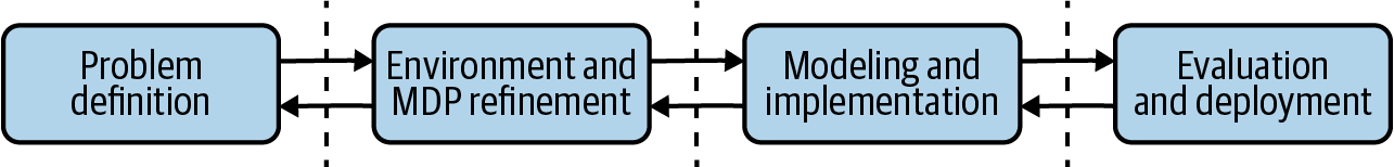
Figure 9-2. A diagram of the four main phases of an RL project.
In an ML project, it is unlikely that you have the ability to dramatically alter the problem definition. You can probably tinker with the performance specification, for example, but fundamentally the problem you are trying to solve is defined by the business. Then you would search for and locate any data that already exists within the business, get permission to use it, and put the technology in place to access it. If you don’t have any data, then you can try to gather new data or use an external source. Once you have the data at your disposal you would spend time analyzing, understanding, cleaning, and augmenting to help solve the problem. This represents the first two boxes of the data science process.
In RL the situation is quite different, even perverse at times. First you are given a business challenge. The problem is strategic, at a higher level of abstraction compared to “normal” data science problems, and it has a real-life definition of success like profit, number of subscribers, or clicks. Then you, yes you, take that definition of success and carefully engineer the problem to fit into an MDP and design the reward function. Until there is an inverse RL (see “Inverse RL”) algorithm that works in every situation, you will need to design the reward yourself. This is a big burden to place on your shoulders. You have the power to decide how to quantify performance, in real terms. In one sense this is great, because it directly exposes how the project affects the business in human-readable terms like lives saved (not accuracy or F1-score, for example). But this also places more burden on the engineer. Imagine a strategic-level agent that chooses the direction of the business and it leads to a bad result. Historically, this risk is carried by the executives in your company—hence the girth of the paycheck—but in the future it will be delegated to algorithms like RL, which are designed by engineers. I haven’t seen any evidence of how this is going to affect the hierarchical control structures present in so many companies but I anticipate that there will be a shakeup. Shareholders pay for productivity and when productivity is driven by the engineers that design the algorithms, does that also mean they run the company?
The next phase in the process is to decide how best to learn. In machine learning you only need to iterate on the data you have. But in RL, because it relies on interaction and sequential decisions, you will never have all the data you need to generate realistic rollouts. In the vast majority of cases it makes sense to build simulations to speed up the development feedback cycle, rather than use a live environment. Once you have a viable solution then you can roll out to real life.
Notice the difference here. Either you are generating artificial observations or you don’t have real data until you actively use your algorithm. If someone said to me that I had to deploy my fancy deep learning model into production before collecting any data, I’d probably cry a little inside.
But this is precisely the situation in RL and what makes state, action, and reward engineering so important. You can’t hope to build a robust solution unless you fully understand your state and actions and how they affect the reward. Trying to throw deep learning at a problem you don’t understand is like buying a $1,000 golf club and expecting to become a golf pro.
There’s more, too, which I discuss throughout this chapter. But I want to emphasize that although there are similarities and transferable skills, RL is a totally different beast. The first two boxes in Figure 9-2, problem definition and environment/MDP refinement, I discuss in this chapter. I will leave the final two boxes until the next chapter.
Problem Definition: What Is an RL Project?
I think by now you have a fairly good idea about the definition of RL, but I want to spend this section talking about applying RL to everyday challenges. To recap, you should base your model on a Markov decision process (MDP, see Chapter 2 and “Rethinking the MDP”). The problem should have unique states, which may be discrete or continuous—I find that it often helps to think of discrete states, even if it is continuous. In each state there should be some probability of transitioning to another state (or itself). And an action should alter the state of the environment.
Although this definition captures nearly everything, I find it intuitively difficult to think in terms of states and transition probabilities. So instead I will try to paint a different picture.
RL Problems Are Sequential
RL problems are sequential; an RL agent optimizes trajectories over several steps. This alone separates RL from ML; the paradigm of choice for single-step decision making. ML cannot optimize decisions for a long-term reward. This is crucial in many business challenges. I don’t think any CEO with an inkling of humanity would squeeze a prospect for every penny right now. Instead, they know that managing the relationship and managing how and when the sales that are made to optimize for the long-term support of the customer is the best route toward a sustainable business.
This philosophy maps directly to how you would solve industrial, customer-centric problems. You shouldn’t be using ML models to optimize your ad placement or recommend which product to buy because they optimize for the wrong thing. Like a voracious toddler, they can’t see the bigger picture. ML models are trained to make the best possible decision at the time, irrespective of the future consequences. For example, ML models are very capable of optimizing product recommendations, but they might include the product equivalent of click-bait: products which get lots of clicks but are ultimately disappointing. Over time, a myopic view will likely annoy users and could ultimately hurt profit, retention, or other important business metrics.
RL algorithms are perfectly suited to situations where you can see that there are multiple decisions to be made, or where the environment doesn’t reset once you’ve made a decision. This opens up a massive range of possibilities, some of which you saw in “RL Applications”. These may be new problems or problems that already have a partial solution with ML. In a sense, a problem that has already been partially solved is a better one than a new project, because it’s likely that engineers are already very familiar with the domain and the data. But be cognizant that initial RL results may produce worse results in the short term while algorithms are improved. Visit the accompanying website to get more application insipration.
RL Problems Are Strategic
I like to think of software engineering as a way of automating processes and machine learning can automate decisions. RL can automate strategies.
Figure 9-3 hammers this idea home. Modern businesses are made of three core functions. Businesses have a plethora of processes, from performance reviews to how to use the printer. Enacting of any one of these processes is rarely valuable, but they tend to occur often. Because of the frequency and the fact it takes time and therefore money for a human to perform this process, it makes sense to automate the process in software.
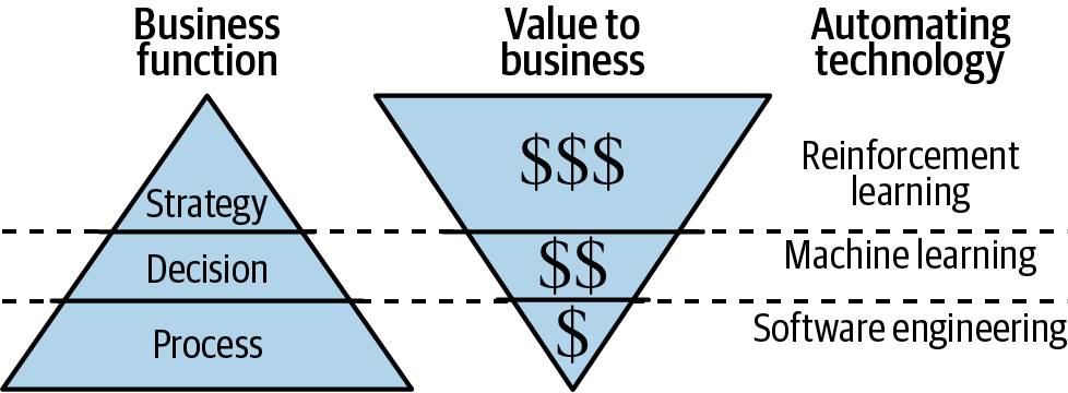
Figure 9-3. A depiction of the different functions of a modern business, the value of each action in that function, and the technology that maps to the function.
Business decisions are rarer than business processes, but they still happen fairly often. Making the decision to perform CPR, phone a warm prospect, or block a suspicious looking transaction can save lives/be profitable/prevent fraud. All of these challenges can be solved using machine learning. These actions are quantifiably valuable, but like I said previously, they have a limited life span. They intentionally focus on the single transitive event. Decisions need processes in place to make them possible.
Business strategies form the heart of the company. They happen rarely, primarily because there are limited numbers of people (or one) designing and implementing the strategy. They are closely held secrets and direct a multitude of future people, decisions, and processes. They have wide-reaching consequences, like the healthcare for a nation or the annual profits of the company. This is why optimal strategies are so valuable and why RL is so important.
Imagine being able to entrust the running of your company/healthcare/country to RL. How does that sound? What do you think?
You might suggest that this is a pipe dream, but I assure you it is not. Taxation is being tackled with MARL.1 Healthcare use cases are obvious and there are thousands of references.2 And companies must automate to become more competitive, which is nothing new—companies have been automating for over a century now.
The future, therefore, is in the hands of the engineers, the people who know how to build, adapt, and constrain algorithms to be robust, useful, and above all, safe.
Low-Level RL Indicators
The previous two suggestions, that RL problems are sequential and strategic, are high level. On a lower level you should be looking for individual components of the problem.
An entity
Look for entities, which are concrete things or people, that interact with the environment. Depending on the problem, the entity could sit on both sides of the environment interface. For example, a person viewing a recommendation is an entity but they are part of the environment. Other times people are simulated agents, like in the taxation example.
An environment
The environment should be, in the language of domain-driven design, a bounded context. It should be an interface that encapsulates all of the complexities of the situation. You should not care whether behind the interface there is a simulation or real life; the data at the interface should be the same. Beware of making an environment too big or too complex, because this impacts the solvability of the problem. Splitting or simplifying the environment makes it easer to work with.
A state
The easiest way to spot state is to observe or imagine what happens when the state changes. You might not think of it as a change, but look carefully. The price of a stock changes because the underlying state of all investors changes. The state of a robot changes because it has moved from position A to position B. After showing a recommendation your target’s state may have changed from “ignore recommendation” to “click on the recommendation.”
What can you observe about the environment (which may include entities)? What are the most pertinent and informative features? Like in ML, you want to be careful to only include clean, informative, uncorrelated features. You can add, remove, or augment these features as you wish but tend toward minimizing the number of features if possible, to reduce the exploration space, improve computational efficiency, and improve robustness. Don’t forget that you can merge contextual information from other sources, like the time of day or the weather.
The domain of the state can vary dramatically depending on the application. For example, it could be images, matrices representing geospatial grids, scalars representing sensor readings, snippets of text, items in a shopping cart, browser history, and more. Bear in mind that from the perspective of an agent, the state may be uncertain or hidden. Remind yourself often that the agent is not seeing what you can see, because you have the benefit of an oracle’s view of the problem.
An action
What happens to the environment when you apply an action? The internal state of an environment should have the potential to change (it may not, because the action was to stay put or it was a bad one) when you apply an action. Ideally you want to observe that state change and if you don’t, consider looking for observations that expose this information. Again, try to limit the number of actions to reduce the exploration space.
Quantify success or failure
In this environment, how would you define success or failure? Can you think of a way to quantify that? The value should map to the problem definition and use units that are understandable to both you and your stakeholders. If you are working to improve profits, then quantify in terms of monetary value. If you are trying to improve the click rate of something, go back and try to find a cash amount for that click. Think about the real reason why your client/boss/stakeholder is interested in you doing this project. How can you quantify the results in terminology they understand and appreciate?
Types of Learning
The goal of an agent is to learn an optimal policy. The rest of this book investigates how an agent learns, through a variety of value-based and policy gradient–based algorithms. But what about when it learns?
Online learning
The overwhelming majority of examples, literature, blog posts, and frameworks all assume that your agent is learning online. This is where your agent interacts with a real or simulated environment and learns at the same time. So far in this book I have only considered this regime. One of the major problems with this approach is the sample efficiency, the number of interactions with an environment required to learn an optimal policy. In the previous couple of decades researchers have been chasing sample efficiency by improving exploration and learning guarantees. But fundamentally there is always going to be an overhead for exploration, sampling delays due to stochastic approximation, and the all important stability issues. Only recently have they begun to consider learning from logs.
Offline or batch learning
Until quite recently, it was thought that all learning had to be performed online because of the inherent coupling between the action of an agent and the reaction of an environment.3 But researchers found that it was possible to learn from a batch of stored data, like data in a replay buffer. Because this data has no further interaction with the environment it is also known as learning offline or in batches. Figure 9-4 presents the idea. First, data is generated online using a policy (possibly random) and saved in a buffer. Offline, a new policy is trained upon the data in the buffer. The new policy is then deployed for use.
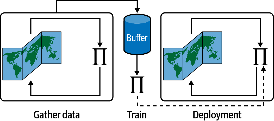
Figure 9-4. Batch reinforcement learning.
The primary benefit of learning offline is the increase in sample efficiency. You can capture or log a set of data and use it to train models as many times as you like with zero impact on the environment. This is an incredibly important feature in many domains where collecting new samples is expensive or unsafe.
But hang on. If I collect and train upon a static snapshot of data, then isn’t this pure supervised learning? The answer is yes, kind of. It is supervised in the sense that you have a batch of data with labeled transitions and rewards. But this doesn’t mean you can use any old regression or classification algorithm. The data is (assumed to be) generated by an MDP and therefore the algorithms designed to find optimal policies for MDPs are still useful. The major difference is that they can no longer explore.
If an agent can’t explore, then it can’t attempt to improve the policy by “filling in the gaps,” which was the primary reason for rapid advances in RL over the past decade. A similar argument is that it prevents the agent from asking counterfactual questions about the action. Again, this is a theoretical method to provide more robust policies by allowing them to ask “what if” questions. Fundamentally, the distribution of the training data (for state, actions, and rewards) is different than that observed at deployment. Imagine how that affects a typical supervised learning algorithm.
In principle, any off-policy RL algorithm could be used as an offline RL algorithm, by removing the exploration part from the algorithm. However, this is problematic in practice for a number of reasons. Value methods struggle because they rely on accurate value estimates. But many of the states or actions will not be present in the buffer and therefore estimates will be inaccurate at best. Policy gradient methods struggle because of the distribution shift, which at best produces gradients that point in the wrong direction and at worst blow up. These problems get worse when you use overly specified models like deep learning.4
At the time of this writing, researchers are working hard to solve these problems to open up the next large gains in sample efficiency. One avenue of research is to further refine the stability guarantees of basic RL algorithms so that they don’t misbehave when encountering unstable distributions or undersampled states or actions. Better theoretical guarantees when using deep learning is an obvious avenue that would dramatically improve the situation. Other approaches are attempting to use techniques like imitation learning to lean policies that generate positive rewards.5 An even simpler approach is to train an autoencoder upon the buffer to create a simulated environment that agents can explore in.6 In practice these techniques are already being applied and are showing impressive results, especially in robotics.7 From a practical perspective, then, you might find the DeepMind RL Unplugged benchmark a useful tool to find or prototype ideas.8
Concurrent learning
The literature contains a mix of learning techniques that fall somewhere between multi-agent RL (MARL) and multiprocess frameworks, but are interesting enough to mention here.
The length of your feedback cycles are dictated by the complexity of the problem; the harder the challenge, the longer it takes to solve. This is partially caused by increasing model complexities, but primarily it is an exploration problem. Large state and action spaces need more exploration to “fill in the gaps.”
Many researchers have concentrated on improving exploration in the single-agent case, which has worked wonders. But that only scales to a point. Ultimately an agent still needs to visit all of the state-action space. One option is to run multiple agents at the same time (see “Scaling RL”), but if they are using the same exploration algorithm then they can tend to explore the same space, again negating the efficiency as the state-action space is scaled up.
Instead, why not explore concurrently, where teams of agents have the joint task of exploring the state-action space. Beware that this term is overloaded, though; researchers have used the word concurrent to mean anything from cooperative MARL to concurrent programming for RL.9,10 I use the term to denote the goal of performing coordinated exploration of the same environment, first suggested in 2013.11
The implementation of this idea is somewhat domain dependent. As one example, many companies are interacting with thousands or millions of customers in parallel and are trying to maximize a reward local to that customer, like lifetime value or loyalty. But these customers reside within the confines of the same environment; a company only has a limited set of in-stock products and you have roughly the same demographic information for each customer. The learnings from one customer should be transferred to others, so this implies either centralized learning or at least parameter sharing.
I don’t think there is one right answer because there are many small challenges that need unique adaptations. Like what would happen if you introduced the ability to retarget customers with emails or ads? This would improve the performance metrics but the rewards may be delayed. So you would have to build in the capacity to “skip” actions and deal with the partial observability.
Dimakopoulou and Van Roy formalized this idea in 2018 and proved that coordinated exploration could both increase learning speed and scale to large numbers of agents.12 Their solution is surprisingly simple: make sure each agent has a random seed that maximizes exploration. The benefit of this approach is you can use standard RL algorithms and each agent is independently committed to seeking out optimal performance. It also adapts well to new data because starting conditions are repeatedly randomized. The challenge, however, is that the optimal seed sampling technique is different for every problem.
In concurrent learning then, agents are independent and do not interact. Agents may have different views of the environment, like different customers have different views of your products. Despite the different name, this is very similar to MARL with centralized learning. So if you are working on a problem that fits this description, then make sure you research MARL as well as concurrent RL.
Reset-free learning
Included in the vast majority of examples and algorithms is the implicit use of “episodes,” which imply that environments can be “reset.” This makes sense for some environments where the starting position is known, fixed, or easily identifiable. But real life doesn’t allow “do-overs,” even though sometimes I wish it would, and would require omnipotent oversight. To avoid an Orwellian version of the film Groundhog Day, many applications need some way of not specifying a reset.
Early solutions suggested that agents could learn how to reset.13 Agents are in control of their actions so you can store previous actions in a buffer. To get back to the starting point you can “undo” those actions. This works in many domains because action spaces have a natural opposite. But action uncertainties and unnatural “undos” prevent this approach being generally applicable.
Another idea is to predict when terminations or resets or unsafe behavior is going to occur and stop it before it happens.14 But again this requires oversight, so another suggestion is to learn a function to predict when resets will occur as part of the learning itself.15 As you can see from the vocabulary this has hints of meta-learning. But none of these approaches is truly reset free; why not eliminate resets entirely?
You could, technically, never reset and use a discounting factor of less than one to prevent value estimates tending toward infinity. But the reset is more important than you realize. It allows agents to have a fresh start, like when you quit your boring job and start an exciting career in engineering. It is very easy for exploring agents to get stuck and spend significant time in similar states. The only way to get out of a rut is for someone or something to give it a kick. A reset is a perfect solution to this problem because it gives the agent another chance to try a different path.
A related problem is when an agent is able to reach a goal or a global optimum, then the best next action is to stay put, gorging on the goal. Again, you need a reset or a kick to explore more of the suboptimal state to make the policy more robust.
So rather than learning how to reset, maybe it is better to learn how to encourage the agent away from the goal and away from regions it can get stuck. Or provide a simple controller to shuffle the environment like Zhu et al., which results in robust robotic policies with no resets.16
To conclude, reset-free learning is possible in some simple applications but it’s quite likely that your agents will get stuck. At some point you will need to consider whether you are able to manipulate your environment to move the agent to a different state. You might also be able to get the agent to move itself to a different state. Again, different problem domains will have different solutions.
RL Engineering and Refinement
RL problems, like any engineering problem, have high-level and low-level aspects. Changing the high-level design impacts the low-level implementation. For lack of a better term, I denote the high-level analysis and design as architectural concerns. These include refining the model of the Markov decision process, defining the interfaces, defining interactions between components, and how the agent will learn. These decisions impact the implementation, or engineering details.
I’ve talked a lot already about high-level architectural aspects, so in this section I want to discuss the implementation details. I endeavor to cover as many of the main concerns as possible, but many implementation details are domain and problem specific. In general, I recommend that you search the literature to find relevant examples and then scour the implementation details for interesting tidbits. These details, often glossed over in the researcher’s account, offer vital insight into what works and what doesn’t.
Process
Before I dive into the details I think it is worth explaining how I perform this engineering work in general terms. I find that most tasks in engineering, irrespective of the abstraction level, tend to follow some variant of the the observe, orient, decide, act (OODA) loop. What is ostensibly the scientific method, the OODA loop is a simple, four-step approach to tackling any problem, popularized by the American military. The idea is that you can iterate on that loop to utilize context and make a quick decision, while appreciating that decisions may change as more information becomes available. Figure 9-5 shows this loop in engineering terms, where I suggest the words analysis, design, implementation, and evaluation are more appropriate, but they amount to the same thing.
The most important aspect is that this is a never-ending process. On each iteration of the loop you evaluate where you are and if that is not good enough, you analyze where improvements could be made. You then pick the next best improvement and implement that.
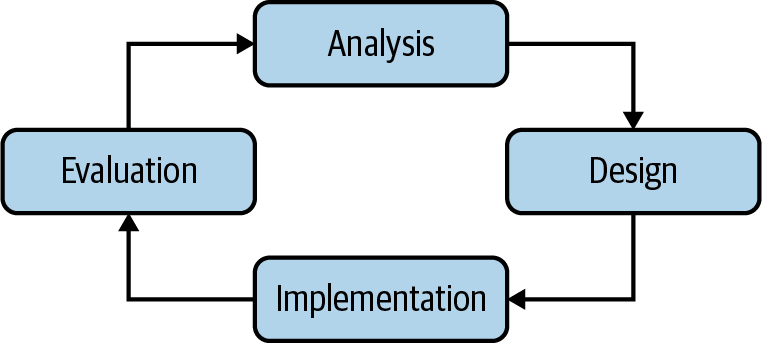
Figure 9-5. The process of RL refinement.
No one single improvement will ever be enough and there is always one more improvement that you could make. You have to be careful not to get stuck in this loop, and you can do that by remembering the Pareto distribution: 80% of the solution will take 20% of the time and vice versa. Consider if implementing that last 20% is really worth it, given all the other value you could be providing with that time.
Environment Engineering
I find that the most productive first step of an RL project is to create an environment. Throughout this book I use this term to denote an abstraction of the world that the agent operates within. It is the interface between what actually happens and what the agent wants (see “Reinforcement Learning”).
But now I am specifically talking about the implementation of this interface. Whether you are working in real life submitting real trades or you are creating a simulation of a wind turbine, you need an implementation of the environment interface.
The benefit of concentrating on this first is that you will become intimately acquainted with the data. This maps to the “data understanding” step in the CRISP-DM model. Understanding your environment is crucial for efficiently solving industrial challenges. If you don’t, what tends to happen is what I call the “improvement shotgun.” By throwing a bunch of different ideas at the problem you will probably find one that hits the target, but most will miss. This type of work is not productive, efficient, or intelligent.
Instead, understand the environment fully, pose scientifically and engineeringly—yes, apparently that is a word—robust questions, and implement functionality that answers those questions. Over time you will gain insight into the problem and you will be able to explain why improvements are important, not just state that they are.
Implementation
OpenAI’s Gym has organically become the de facto environment interface in the RL community.17 In fact, it’s one of the most cited RL papers of all time. You’ve probably come across it before, but just in case you haven’t, a Gym is a Python framework for expressing environments. It exposes useful primitives like definitions for action and state space representation and enforces a simple set of functionality via an interface that should suit most applications. It also comes with a big set of example environments that are used throughout the internet as toy examples.
From an industrial perspective, the interface is a great way to model your problem and help refine your MDP. And because it is so popular, it is likely that you can rapidly test different algorithms because the majority expect the Gym interface.
Tip
I’m not going to go through a detailed example of an implementation, because it is out of the scope of this book, but you can find many great examples from a quick search or visiting the Gym GitHub website.
Simulation
A simulation is supposed to capture the most important aspects of a real-life problem. Simulations are not intended to be perfect representations, although many people, researchers, and businesses invest vast amounts of time making simulations more realistic. The benefit of having a simulation is that it is easier, cheaper, and quicker to operate within the confines of a simulation than it is in real life. This reduces the length of the developmental feedback cycles and increases productivity. But the precise benefits depend on the problem; sometimes learning in real life is easier and simpler than building a simulation.
You should first search to see if someone has already attempted to build a simulation. Understanding the fundamental aspects of the problem, the physics, biology, or chemistry, is often more difficult than solving the problem, although building a simulation will certainly improve your knowledge about the subject, so it might be worthwhile for that reason alone. Many commercial simulators like MuJoCo or Unity are available, but come with a commercial price tag. You will have to decide whether the cost is worth the money for your problem. In general I recommend evaluating whether the simulation is a competitive differentiator for your business or product. If it is, it may be worth investing in development; if not, save yourself a lot of time and buy off-the-shelf. And I have found that these vendors are immensely helpful and professional, so ask them for help. It is in their interest for your idea or business to succeed, because that means future revenue for them.
If you do decide to implement the simulator yourself then you will need to build models to simulate the problem and decide which aspects to expose. This is where MDP design plays a crucial role. In general, you should try to expose the same aspects of the problem that can be observed in real life. Otherwise, when you try to transfer your learnings to real life you will find that your agent doesn’t behave as you expect.
Similarly, many researchers attempt to take models trained in simulation and apply them to real-life tasks. This is certainly possible, but is entirely defined by how representative the simulation is. If this is your intention, then you should implicitly couple the implementations of the simulation and real life. The vast majority of algorithms and models don’t like it when you change the underlying state or action space.
Simulations are perfect for proof-of-concept projects, to validate that an idea is technically viable. But be careful to not place too much hope on the simulation because there is no guarantee that the policy your agent has derived is possible in real life. It is eminently possible that real-life projects can fail spectacularly even though simulations work perfectly. More often than not the simulation misses some crucial aspect or information.
Interacting with real life
If your experience with the simulation is encouraging, or you have decided that it is easier to skip the simulation, then the next step is to build another (Gym) interface to interact with real life. The development of such an implementation is often much easier, because you don’t need to understand and implement the underlying mechanics; nature does that for you. But adapting your algorithms to suit the problem is utterly dependent on understanding and controlling the data.
The primary concerns of the real-life implementation consist of the operational aspects, things like scaling, monitoring, availability, and so on. But architecture and design still plays an important part. For example, in real life there are obvious safety concerns that are not present in a simulation. In some domains a significant amount of time must be invested in ensuring safe and reliable operation. Other common problems include partial observability, which doesn’t exist in an omnipotent simulation, and excessive amounts of stochasticity; you would have thought that motors move to the position you tell them to, but often this is not the case.
I don’t think this small section sufficiently expresses the amount of engineering time that can go into real-world implementations. Of course, implementations are wildly domain specific, but the main problem is that this work is pretty much pure research. It is hard to accurately estimate how long the work will take, because neither you nor anyone else in the world has tackled this exact problem before. You are a digital explorer. Remember to remind your project managers of this fact. And remember the process from the start of this chapter. Start simple. Life is hard enough without you making it harder.
State Engineering or State Representation Learning
In data science, feature engineering is the art/act of improving raw data to make it more informative and representative of the task at hand. In general, more informative features make the problem easier to solve. A significant amount of time after a proof of concept is spent cleaning, removing, and adding features to improve performance and make the solution more robust.
I like to use similar terminology to refer to the engineering of the state, although I haven’t seen it used much elsewhere. State engineering, often called state representation learning, is a collection of techniques that aim to improve how the observations represent the state. In other words, the goal is to engineer better state representations. There is no right way of doing this, however, so you are primarily guided by metrics like performance and robustness.
Although there are parallels, this isn’t feature engineering. The goal is not to solve the problem by providing simpler, more informative features. The goal is to create the best representation of the state of the environment as you can, then let the policy solve the problem. The reason for this is that in most industrial challenges, it is very unlikely that you are capable of crafting features that can compete with an optimal multistep policy. Of course, if you can, then you should consider using standard supervised learning techniques instead.
Like in feature engineering, domain expertise is important. The addition of a seemingly simple feature can dramatically improve performance, far more than trying different algorithms. For example, Kalashnikov et al. found that in their robotics experiments that used images as the state representation, adding a simple “height of gripper” measurement improved the robot’s ability to pick up unseen objects by a whopping 12%.19 This goes to show that even though researchers are always trying to learn from pixels, simple, reliable measurements of the ground truth are far better state representations.
Note that many papers and articles on the internet bundle both the state engineering and policy/action engineering into the same bucket. But I do consider them separate tasks because the goal of state engineering is to concentrate on better representations of the state, not improve how the policy generates actions.
Learning forward models
In some cases it may be possible to access ground truth temporarily, in a highly instrumented laboratory experiment, for example, but not in general. You can build a supervised model to predict the state from the observations and ship that out to the in-field agents. This is also called learning a forward model.
Constraints
Constraining the state space helps to limit the amount of exploration required by the agent. In general, policies improve when states have repeated visits, so limiting the number of states speeds up learning.
Apply constraints by using priors, information that is known to be true, formally defined by a probability distribution. For example, if you know that features should be strictly positive, then ensure your policy knows that and doesn’t attempt to reach those states.
Transformation (dimensionality reduction, autoencoders, and world models)
Dimensionality reduction is a task in data science where you try to reduce the number of features without removing information. Traditional techniques are useful in RL too. Using principal component analysis, for example, reduces the state space and therefore reduces learning time.20
But the crown jewels of state engineering are the various incarnations of autoencoders to reconstruct the observation. The idea is simple: given a set of observations, train a neural network to form an internal representation and regenerate the input. Then you tap into that internal representation and use it as your new state.
Typically, implementations attempt to reduce the dimensionality of the input by using a neural architecture that progressively compresses the state space. This constraint tends to force the network to learn higher-level abstractions and hopefully, an important state representation. However, there are suggestions that increasing the dimensionality can improve performance.21 I remain somewhat skeptical of this claim as it actively encourages overfitting.
Learning representations of individual observations is one thing, but MDPs are sequential, therefore there are important temporal features locked away. A new class of MDP-inspired autoencoders is beginning to treat this more like a prediction problem. Given an ordered set of observations, these autoencoders attempt to predict what happens in the future. This forces the autoencoder to learn temporal features as well as stateful features. The particular implementation differs between domains, but the idea remains the same.22,23
The term world models, after the paper with the same name, refers to the goal of attempting to build a model of an environment from offline data, so that the agent can interact as if it was online. This idea is obviously important for practical implementations where it is hard to learn on live data and so the term has become popular to describe any method that attempts to model an environment.24 Ha and Schmidhuber deserve extra kudos because of their excellent interactive version of their paper. I consider this work to be a specific implementation of state engineering, which may or may not be useful depending on your situation, but it is a very useful tool to help segment the RL process.
These techniques can be complicated by MDP issues like partial observability, but in general autoencoder research can be directly applied to RL problems. If this is important for your application then I recommend you dig into these papers. Frameworks are also beginning to see the value in state representation, like SRL-zoo, a collection of representation learning methods targeting PyTorch, which you might find useful.
Policy Engineering
An RL policy is responsible for mapping a representation of the state to an action. Although this sounds simple, in practice you need to make careful decisions about the function that implements this mapping. Like in machine learning, the choice of function defines the limits of performance and the robustness of the policy. It also impacts learning performance, too; using nonlinear policies can cause divergence and generally take much longer to train.
I generalize this work under the banner of policy engineering, where the goal is to design a policy that best solves a problem given a set of constraints. The vast majority of the RL literature is dedicated to finding improved ways of defining policies or improving their theoretical guarantees.
The policy is fundamentally limited by the Bellman update, so unless there is a major theoretical shift, all policies have a similar aim. Researchers introduce novelty by affixing new ways to represent state, improve exploration, or penalize some other constraint. Underneath, all RL algorithms are value-based or policy-based.
Given this similarity between all algorithms I visualize a policy as having three distinct tasks, like in Figure 9-6. First it has to convert the representation of state into a format that can be used by an internal model. The internal model is the decision engine, learning whatever it needs to learn to be able to convert state to possible actions. A policy has to explore and you have a lot of control over that process. Finally, the policy has to convert the hidden representation into an action that is suitable for the environment.
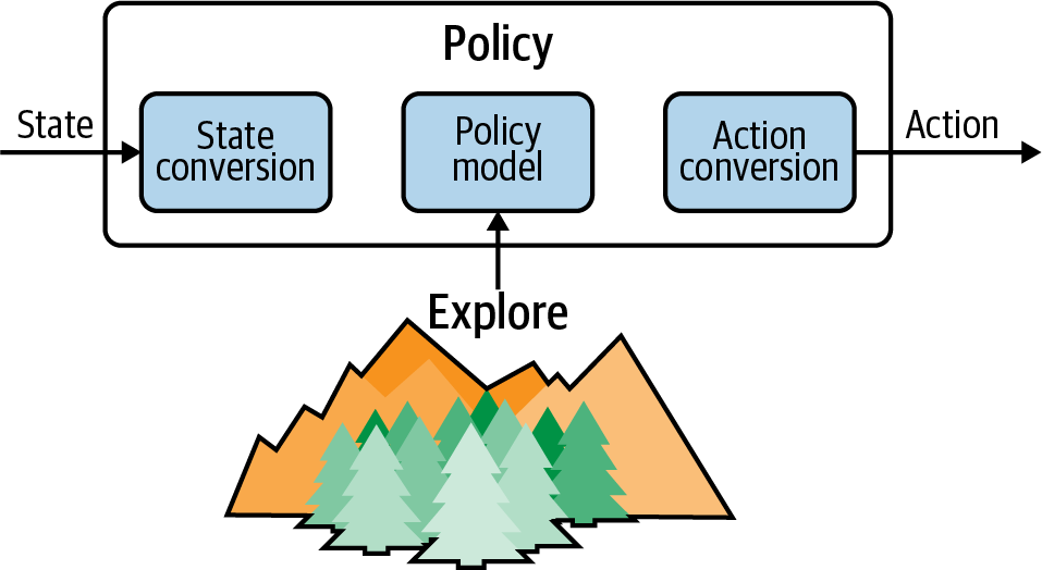
Figure 9-6. A depiction of the three phases of a policy.
The engineering challenge is to design functions to perform these three phases in an efficient and robust way. The definition of the policy model has been the subject of most of this book. In the following subsections I describe how to use discrete or continuous states and actions.
Discrete states
A discrete feature is permitted to only take certain values, but can have an infinite range. The vast majority of data is received in a form quantized by analog-to-digital converters, so you can consider most data to be discrete. But in practice when people say “discrete space” they typically mean an integer-based state space, where state can take only integer values. Most of the time quantized data is converted to a float and is considered continuous.
Discrete state inputs are useful because of their simplicity. There are fewer states that an agent has to explore and therefore training performance and time can be reduced, even predicted. Problems with smaller state spaces will converge faster than larger ones.
A discrete state space is any GridWorld-like environment. Geospatial problems are a good example. Even though positions could be encoded by continuous measures like latitude and longitude, it is often computationally and intuitively simpler to convert a map into a grid, like Chaudhari et al. did when optimizing ride-share routing policies in the city of New York.25
Problems with discrete state spaces are considered to be easier to solve, mainly because it is so easy to debug and visualize. Discrete domains are often easy to reason about, which makes it possible to make accurate theoretical priors and baselines. You can directly compare policies to these assumptions, which makes it easy to monitor training progress and fix problems as they arise. Another benefit is that value functions can be stored in a dictionary or lookup table, so you can leverage industrially robust technology like databases.
But the most important benefit is that discrete spaces are fixed; there is no chance of any “in-between” state, so there is no need for any approximation of any kind. This means you can use basic Q-learning. Using a simpler, more theoretically robust algorithm like Q-learning leads to simpler and more robust implementations, a very important factor when using these models in production.
The problem, however, is that naturally occurring discrete states are uncommon. In most implementations the engineer has forced the discrete state upon the problem to obtain the aforementioned benefits. This arbitrary discretization is likely to be sub-optimal at best and causes a loss of information detail. Even though the arguments for discrete state spaces are enticing, it is unlikely that they yield the best performance. In the previous example, for instance, the diameter of each cell in New York’s grid was about 2 miles. Even after optimizing the positioning of ride-share vehicles, they could end up being 2 miles from their customer.
Continuous states
A continuous feature is an infinite set of real values. They may be bounded, but there is no “step” between neighboring values. An example could be the speed of an autonomous vehicle or the temperature of a forge. Continuous state spaces are considered to be slightly more difficult to work with than discrete spaces because this leads to an infinite number of potential states, which makes it impossible to use a simple lookup table, for example.
Policies of continuous states have to be able to predict the best next action or value for a given state, which means that the policies must approximate, rather than expect known states. You can provide an approximation using any standard machine learning technique, but functional approximators are most common. Neural networks are increasingly popular due to the unified approach and tooling.
The main worry about continuous state spaces is that they are only provably convergent when using linear approximators. As of 2020, no convergence proofs exist for nonlinear approximators, which means that any “deep” algorithm isn’t guaranteed to converge, even if it is a good model, although empirical evidence suggests they do. Linear approximations can model a significant amount of complexity via domain transformations. Simplicity, stability, and configurable amounts of complexity mean that like in machine learning, linear methods are very useful. In general, there are three ways to provide an approximation:
- Linear approximations
-
Learning a set of linear weights directly based upon the input features is possibly one of the simplest approaches to deal with continuous states. This is effectively the same as linear regression. You can also improve the quality of the regression through any standard linear regression extension, like those that reduce the influence of outliers, for example. A linear policy is provably convergent.
- Nonparametric approximations
-
You can use a classification-like model to predict values, if that makes sense. For example, nearest neighbor and tree-based algorithms are capable of providing robust, scalable predictions. Again, their simplicity and popularity has led to a wide range of off-the-shelf, robust industrial implementations, which you can leverage to make your implementation more scalable and robust. There is no guarantee that nonparametric policies will converge.
- Nonlinear approximation
-
Nonlinear approximations provide a flexible amount of complexity in a uniform package: neural networks. You can control the amount of complexity through the architecture of the network. Neural networks have produced state-of-the-art results in many domains so it would be wise to evaluate them in your problem. There is no guarantee that nonlinear policies will converge.
The provable convergence guarantees are a strong feature of linear approximations. And you can obtain a surprising amount of model complexity by transforming the data before passing to the linear approximation. The following below is a selection of popular techniques to increase model complexity while maintaining the simplicity and guarantees of linear methods:
- Polynomial basis
-
A polynomial expansion is the generation of all possible combinations of features up to a specified power. Polynomials represent curves in value space, which enables slightly more complexity over linear methods.
- Fourier basis
-
Fourier expansions generate oscillations in value space. These oscillations can be combined in arbitrary ways to generate complex shapes, similar to how sounds are comprised of tonal overlays. Fourier bases are complete, in the sense that they can approximate any (well-behaved) function for a given level of complexity, controlled by the order of the basis function. They work well in a range of domains.26 The Fourier basis struggles in environments with discontinuities, like the
Cliffworldenvironment, however. - Radial basis
-
Radial basis functions are often Gaussian-shaped transformations (other radial bases exist) that measure the distance between the state and the center of the basis, relative to the basis’s width. In other words, these are parameterized Gaussian-like shapes that can be moved and resized to approximate the value function. The main problem with radial basis functions (and other tiling schemes) is that you have to choose the width of the basis, which effectively fixes the amount of “smoothing.” Optimal trajectories tend to produce “spikes” in the value function so you end up having to use quite narrow widths, which can lead to problematic local optima. Despite this radial basis functions are useful because the width hyperparameter provides a simple and effective way to control the “amount of complexity.”
- Other transforms
-
Signal processing provides a wide range of other transformations that could be applied to generate different feature characteristics, like the Hilbert or Wavelet transforms, for example. But they are not so popular, typically because most RL researchers have a mathematical or machine learning background. Those with an electronics background, for example, would be more than happy to use these “traditional” techniques.
For more details about linear transformations, see the extra resources in “Further Reading”.
Converting to discrete states
You may want to consider discretizing your domain. Converting continuous states is especially common where there are natural grid-like representations of a domain, like on a map. The main benefit of discretizing is that it might remove the need for a function approximator, because of the fixed size of the state space. This means that simple, fast, and robust Q-learning-based algorithms can be used. Even if you do still need a function approximator, discretization decreases the apparent resolution of the data, making it much easier for agents to explore and easier for models to fit. This has proven to result in an increase in raw performance for difficult continuous problems like in the Humanoid environment.27 The following list presents an overview of discretization possibilities (more information can be found in “Further Reading”):
- Binning
-
Fix the range of a feature and quantize it into bins, like a histogram. This is simple and easy to comprehend but you lose accuracy. You can place bin boundaries in a range of nonuniform ways, like constant width, constant frequency, or logarithmically, for example.
- Tile coding
-
Map overlapping tiles to a continuous space and set a tile to 1 if the observation is present in that tile’s range. This is similar to binning, but provides increased accuracy due to the overlapping tiles. Tiles are often square, but can be any shape and nonuniformly positioned.
- Hashing
-
When features are unbounded, like IP or email addresses, you can forcibly constrain the features into a limited set of bins without loss of information by hashing (there will still be a loss in accuracy due to binning).
- Supervised methods
-
In some domains you may have labeled data that is important to the RL problem. You might want to consider building a classification model and pass the result into the RL algorithm. There are a wide variety of algorithms suitable for this purpose.28
- Unsupervised methods
-
If you don’t have labels you could use unsupervised machine learning methods, like k-means, to position bins in better locations.29
Mixed state spaces
If you have a mixed state space then you have three options:
-
Unify the state space through conversion
-
Cast the discrete space to a continuous one and continue using continuous techniques
-
Split the state space into separate problems
Options 1 and 2 are self explanatory. The majority of functional approximators will happily work with discretized values, even though it may not be optimal or efficient.
Option 3, however, is interesting. If you can split the state into different components that match bounded contexts in the problem domain, that might indicate that it is more efficient to use submodels or subpolicies. For example, a crude approach could be to separate the continuous and discrete states, feed them into two separate RL algorithms, then combine them into an ensemble.30 As you can see this is touching upon hierarchical RL, so be sure to leverage ideas from there.
Mapping Policies to Action Spaces
Before you attempt to define how a policy specifies actions, take a step back and consider what type of actions would be most suitable for your problem. Ask yourself the following questions:
-
What value types can your actions take? Are they binary? Are they discrete? Are they bounded or unbounded? Are they continuous? Are they mixed?
-
Are simultaneous actions possible? Is it possible to select multiple actions at the same time? Can you iterate faster and interleave single actions to approach selecting multiple actions?
-
When do actions need to be made? Is there a temporal element to action selection?
-
Are there any meta-actions? Can you think of any high-level actions that might help learning or handle the temporal elements?
-
Can you split the actions into subproblems? Are there obvious bounded contexts in your actions? Can these be split into separate problems? Is this a hierarchical problem?
-
Can you view your actions in another way? For example, rather than moving to a continuous-valued position, could you consider a “move forward” action? Or vice versa?
All of these decisions have grave impacts on your work, so be careful when making them. For example, switching an action from continuous to discrete might force you to change algorithms. Or realizing that your agent requires simultaneous actions might make your problem much harder to solve.
Binary actions
Binary actions are possibly the simplest to work with, because they are easy to optimize, visualize, debug, and implement. Policies are expected to output a binary value mapping to the action that they want to choose. In problems where only a single action is allowed, picking the maximum expected return (for value methods) or the action with the highest probability (for policy gradient methods) is a simple implementation.
As seen in “How Does the Temperature Parameter Alter Exploration?”, you can encourage broad exploration by making the policy output probabilities, or values that can be interpreted as probabilities. The agent can then randomly sample from this action space according to the assigned probabilities. For value methods, you can assign the highest probabilities to the highest expected values. I would recommend using advantages, rather than values directly, to avoid bias. An exponential softmax function is recommended to convert values to probabilities. In policy gradient methods you can train the models to predict probabilities directly.
Continuous actions
Continuous actions are very common, like determining the position of a servo or specifying the amount to bid on an ad. In these cases it is most natural to use some kind of approximation function to output a continuous prediction for a given state (just like regression); deterministic policy gradients do this. But researchers have found that modeling the output as a random variable can help exploration. So rather than directly predicting the output value, they predict the mean of a distribution, like a Gaussian. Then a value is sampled from distribution. Other parameters of the distribution, like the standard deviation for the Gaussian, can also be predicted. Then you can set the initial standard deviation at the beginning high, to encourage exploration, and allow the algorithm to shrink it as it learns. I like to think of this as a crude attempt to incorporate probabilistic modeling. Of course this assumes that your actions are normally distributed, which may not be accurate, so think carefully about what distribution you should choose for your actions.
An alternative is to leverage newer methods that are based upon Q-learning, but have been adapted to approximate continuous functions: continuous action Q-learning.31 This is by no means as common as using policy gradient methods but claims to be more efficient.
One final trick that I want to mention, which is helpful in simple examples, is called the dimension scaling trick. When using linear approximators that need to predict multiple outputs, like the mean and standard deviation, you can have distinct parameters for each action and update the parameters for the chosen action individually. This is effectively a dictionary of parameters, where the key is the action and the values are the parameters for the continuous mapping, like the mean and standard deviation.
Hybrid action spaces
Spaces with both discrete and continuous actions are relatively common, like deciding to buy and how much to spend, and can be tricky to deal with. First consider if you can split the problem. If it’s a hierarchical problem, go down that route first. Next consider if you can get away with only continuous or only discrete. You’ll probably lose a little bit of granularity, but it might make it easier to get something up and running.
New algorithms are emerging that learn when to select either a continuous algorithm or a discrete one, depending on the required action space. Parameterized DQN is one such example, but the idea could be applied to any algorithm.32 Another approach called action branching simply creates more heads with different activations and training goals on a neural network, which seems like a nice engineering solution to the problem.33 This multihead architecture also enables simultaneous actions. In a sense this just a handcrafted form of hierarchical RL.
When to perform actions
Here’s a curveball: what about when you want to output no action? That’s actually a lot harder than it sounds, because everything from the Bellman equation to neural network training is set up to expect an action on every step. The Atari games implement frame skipping without really considering how many frames to skip; 4 are just taken as given. But researchers have found that you can optimize the the size of number of skipped frames to improve performance.34
A more generalized approach is to use the options framework, which include a termination condition. These methods learn not only how to act optimally, but also when.35,36 A potentially simpler solution is instead to add an action that causes the agent to repeat previous actions; I have seen this used in robotics to reduce wear and tear on motors. It is also possible to learn to skip as many actions as possible, to reduce costs associated with an action.37
As usual, the best solution is problem dependent. Generally I would recommend staying within the realms of “normal” RL as much as possible, to simplify development.
Massive action spaces
When state spaces become too large you can use state engineering to bring them back down to a reasonable size. But what about when you have massive action spaces, like if you are recommending one of millions of products to a customer? YouTube has items in its corpus, for example.38
Value-based methods like Q-learning struggle because you have to maximize of a set of possible action on every step. The obvious challenge is that when you have continuous actions, the number of actions to maximize over is infinite. But even in discrete settings there can be so many actions that it might take an infeasibly long time to perform that maximization. Policy gradient methods overcome this problem because they sample from a distribution; there is no maximization.
Solutions to this problem include using embeddings to reduce the total number of actions to a space of actions.39 This has instinctive appeal due to the successes of embeddings in other ML challenges, like in natural language processing. If you have action spaces that are similar to problems where embeddings have been successful, then this might be a good approach. Another approach is to treat the maximization as an optimization problem and learn to predict maximal actions.40
A related issue is where you need to select a fixed number of items from within the action space. This presents a combinatorial explosion and is a common enough issue to have attracted research time. There are a wide range approximate solutions like hierarchical models and autoencoders.41,42 A more general solution is to move the complexity in the action space into the state space by inserting fictitious dummy states and using group actions predicted over multiple steps to produce a selection of recommendations.43 A simpler and more robust solution is to assume that users can select a single action. Then you only need to rank and select the top- actions, rather than attempting to decide on what combination of actions is best. This solution has been shown to increase user engagement on YouTube.44
Note
Consider this result in the context that Google (which owns YouTube) has access to one of the most advanced pools of data scientists in the world. This algorithm is competitive with its highly tuned recommendations model that (probably) took teams of highly experienced data scientists many years to perfect. Incredible.
Exploration
Children provide personal and professional inspiration in a range of sometimes surprising ways, like when I’m working on a presentation or a new abstraction I routinely try to explain this to my kids. If I can’t explain it in a way that sounds at least coherent to them, then that’s a signal to me that I need to work harder at improving my message. The book The Illustrated Children’s Guide to Kubernetes is a cute testament to this idea.
Children also provide direction for improvements in exploration. This is necessary because I have spent most of this book explaining that most problems are an exploration problem: complex states, large action spaces, convergence, optima, and so on. All these problems can be improved with better exploration. Recent research has shown that children have an innate ability, at a very early age, to actively explore environments for the sake of knowledge. They can perform simple experiments and test hypotheses. They can weave together multiple sources of information to provide a rich mental model of the world and project this knowledge into novel situations.45
RL algorithms, on the other hand, are primarily driven by error, and learning is almost random. Without a goal, agents would stumble around an environment like an annoying fly that is seemingly incapable of flying back through the open window it came through.
It seems that children tend to operate using an algorithm that approaches depth-first search. They like to follow through with their actions until there is a perceived state that blocks the current path, like a dead end in a maze. Incredibly, this works without any goal, which means they are transferring knowledge about the states from previous experience. When the same children are then presented with a goal, they are able to use the mental map produced by their exploration to dramatically improve the initial search for a goal. Contrast this with current RL algorithms that generally rely on finding a goal by accident.
To this end, there is a large body of work that investigates how to improve exploration, especially in problems that have sparse rewards. But first consider whether you can provide expert guidance in the form of improved algorithms (like replacing -greedy methods with something else) or intermediary rewards (like distance-to-goal measures), or using something like imitation RL to actively guide your agent. Also consider altering your problem definition to make the rewards more frequent. All of these will improve learning speed and/or exploration without resorting to the following methods.
Is intrinsic motivation exploration?
Researchers are trying to solve the problem of exploration by developing human-inspired alternatives to random movement, which leads to a glut of proposals with anthropomorphic names like surprise, curiosity, or empowerment. Despite the cutesy names, exploration methods in humans are far too complex to encode in a simple RL algorithm, so researchers attempt to generate similar behavior through mathematical alterations to the optimization function.
This highlights the problem with all of these methods; there is no right answer. I’m sure you can imagine several mathematical solutions to encourage exploration, like the entropy bonus in the soft actor-critic, but they will never come close to true human-like exploration without prior experience. This is why I think that this field is still young and why words like “curiosity” or “intrinsic motivation” are bad monikers, because they imply that exploration is all about trying new actions. It’s not. Exploration is RL. You use prior knowledge to explore new states, based upon the anticipation of future rewards.
Imagine a classic RL game where your agent is looking at a wall. If it knows anything about walls, it should never explore the states close to the wall, because there is no benefit from doing so. All RL algorithms neglect the simple physical rule that you can’t walk through walls, so they waste time literally banging their head against the wall. But it’s also interesting to note that these assumptions can prevent us from finding unexpected states, like those annoying invisible blocks in the Super Mario series.
So if you want to perform optimal exploration then you need prior experience. I think that transferring knowledge between problems is the key to this problem and unsupervised RL has a potential solution. And counterfactual reasoning will become more important as algorithms begin to start using “libraries” of prior knowledge.
Intrinsic motivation and the methods discussed next are not really about exploration at all. They attempt to improve the cold start problem. When you have zero knowledge with sparse rewards, how can you encourage deep exploration?
Visitation counts (sampling)
One of the simplest ways to improve the efficiency of exploration is to make sure that the agent doesn’t visit a state too many times. Or conversely, encourage the agent to visit infrequently visited states more often. Upper-confidence-bound methods attempt to prevent the agent from visiting states too often (see “Improving the -greedy Algorithm”). Thompson sampling is an optimal sampling technique for this kind of problem and probabilistic random sampling, based upon the value function or policy predictions, can serve as a useful proxy.
Information gain (surprise)
Information gain is used throughout machine learning as a measure of the reduction in entropy. For example, tree-based algorithms use information gain to find splits in feature space that reduce the amount of entropy between classes; a good split makes pure or clean classes, so the information gain is high.46
Many researchers have attempted to use information gain to direct the agent toward regions of greater “surprise.” The major benefit over raw sampling techniques is that they can incorporate internal representations of the policy, rather than relying on external observations of the movement of an agent.
One example of this is variational information maximizing exploration (VIME), which uses the divergence (see “Kullback–Leibler Divergence”) between observed trajectories and those expected by a parameterized model as an addition to the reward function.47 Note the similarity between this idea and thtose discussed in “Trust Region Methods”. This results in exploration that appears to “sweep” through the state space.
State prediction (curiosity or self-reflection)
Curiosity is a human trait that rewards seeking out and finding information that surprises. The previous approach focused upon encouraging surprising trajectories, but you might not want this, because interesting paths are quite likely to lead to a result that is not very surprising at all. Consider if this is important in your problem. For example, you might be searching for new ways of achieving the same result, in which case this would be very useful. In many problems, however, it is the result that is important, not how you got there.
So rather than encouraging different paths, like different routes to school, another solution is to encourage new situations, like going to a different school. One example of this is to create a model that attempts to predict the next state based upon the current state and action, then rewarding according to how wrong the prediction is.48 The problem with this method is that predicting future states is notoriously difficult due to the stochastic and dynamic nature of the environment. If it was that easy, you could use machine learning to solve your problem. So they attempt to model only the parts of the state that affect the agent. They do this by training a neural network that predicts an action from two consecutive states, which creates an internal representation of the policy, and then rewarding based upon the difference between a model that predicts what the internal representation should be and what it actually is after visiting that state. A simpler, similar approach would be to use a delayed autoencoder that compares the hidden representation against that which is observed.
Curious challenges
In the real world, novel states are encountered all the time. Like the previous method suggests, we build long-term models to predict what is novel. That implies that we have also learned how to ignore the noise. Think of when you are driving a car. You have somehow learned how to automatically ignore 99% of the irrelevant information around you and concentrate on the hazards. But put a TV screen or a mobile phone in view and your eyes will be drawn toward it. This promise of seeing something new, at the expense of spotting hazards, is what makes driving with phones or tablets so dangerous.
Researchers have found that a similar problem exists in RL. Figure 9-7 shows a hilarious scenario where a TV was placed upon a wall.49 The state-curiosity-driven agent is perpetually rewarded because it cannot predict what is going to be shown next on TV. Obviously this result is a little contrived; the whole point of these models is to filter out such noise, which should be fairly easy to do if you understand the domain. But in general, researchers need to focus more on improving global exploration, not local.
Figure 9-7. Using observations as a source of surprise can encourage agents to get stuck in noisy states. Adapted from a video by © Deepak Pathak, used under CC BY 2.0 license.
Random embeddings (random distillation networks)
One idea to overcome the “noisy-TV” problem, where agents become fixated with stochastic states, is to use random embeddings. Random distillation networks are a pair of neural networks, one of which is randomly initialized and never touched again. The random network is used to generate random embeddings. A second network is trained to predict the random embeddings. In the work of Burda et al., the error between the random and predicted embedding is used as a “novelty” measure; a greater error means that this type of observation is not well represented in the buffer and therefore should be visited again in the future. This error value is appended to the reward to promote visiting new states.50
The major benefit of this approach is that it is not predicting the next observation; it is just comparing the next observation to its current model of the environment. This means that the stationary view of a stochastic states, like a single image on the TV, can be modeled quite well and therefore the agent is not rewarded for being a “couch potato.”
I find the idea of using a randomly initialized neural network as an embedding hard to fathom. But imagine if your vision was afflicted by some random transformation. Given time your brain would learn to compensate for this and would develop new abstractions; survivors of a stroke have to go through this ordeal. Another benefit is that this architecture is simpler, in the sense that there is only a single network to train. But the exploration is still purely local; it does not promote exploration in depth. Another problem is that it is crucial to have an architecture that produces an effective embedding in the domain. Convolutional neural networks clearly work well in image-based domains, but what about others? These cases need your domain and modeling expertise.51
Distance to novelty (episodic curiosity)
One interesting avenue of research to promote global exploration is to use distance between states as a better measure of novelty. Savinov et al. propose using an experience buffer to record novel states, which are encoded by an embedding. The buffer is cleared at the start of every episode. When an agent happens upon a new state, the distance between the states in the buffer and the current state is estimated. If the new state is within a few environment steps of those in the buffer, it is not novel and is punished. If the new state is further than a few steps away then the agent is rewarded for finding novel states. This encourages agents to seek out new states on an episodic basis.52
Figure 9-8 is a representation of the trajectory followed during one episode. It shows the sign of the reward and when embedded observations were placed in the buffer. You can see that the algorithm has the effect of forcing the agent to keep moving, which promotes depth-first exploration and prevents the agent from becoming a “couch-potato.”
The implementation is quite complex. First, images are converted to hidden embeddings by a convolutional neural network using one-half of a siamese network, which is a neural network architecture used in image matching tasks.53 I don’t like this name but that’s what the literature calls it. Next, the current embedding is compared to all of the embeddings in the buffer, creating a measure of distance to all other observations. Finally, an aggregation is performed to find the distance to next closest state, which represents the novelty of this observation, and is used to calculate the reward.
Figure 9-8. Trajectories from an episode of the DMLab environment with episodic curiosity. The lefthand box shows how the agent was rewarded for that state (green means positive reward, red means negative). The middle box represents when “memories” were added to the episodic buffer. The right box is the first-person view of the agent. Video adapted from Savinov et al.
Exploration conclusions
We know that people explore in depth, using prior knowledge. Transferring that idea to RL is incredibly difficult, because there is no obvious way to direct exploration without breaking the assumptions of an MDP. It feels like there is a gap, one that an MDP cannot fill, where part of the problem is purely supervised, like revising for an exam, but another is entirely opportunistic, like spending time in a different culture.
This is an important problem to solve, because sparse states occur often in RL, due to the nature of goal-driven engineering. Sparse rewards are difficult to work with because they are hard to find. Creating an alternative, pseudoreward that encourages an arbitrary exploration strategy is one solution, but in many problems it is relatively straightforward to manually design rewards to suit your problem (see “Reward Engineering”), or alter the problem definition to make it easier.
Current attempts to automate exploration take a local, episodic view and do not consider global or long-term exploration goals. In fact, researchers have observed that promoting novelty actively encourages dangerous states, like walking along the edge of the cliff, because they are difficult to get close to and are rarely represented in the agent’s past experience.54
All efforts encourage exploration by augmenting the reward function, rather than by guiding action selection. There are clear parallels between this, curriculum learning, and inverse RL that could improve this situation. To be sure, the future of exploration research will be directed toward either altering the fundamental definition of the MDP, by allowing some high-level coordination (thus breaking the Markovian assumption), or incorporating the work of other fields in RL to encourage long-time horizon planning.
Reward Engineering
Designing a reward to solve your problem is arguably the most important task in RL. This is where, as an engineer, it is your job to convert the problem definition into a metric that guides the agent toward a solution. This is incredibly important. Your definition dictates the solution and it is easy to accidentally cause the agent to solve the wrong problem. Figure 9-9 is a great visual example of this happening. An agent in the Unity framework is encouraged to reach a goal and it can use a box to jump over a wall. Instead, because of the slight edge around the environment, the agent has learned to sneak around the side. Despite having a reasonable reward, the agent has learned to exploit the environment in ways that you cannot imagine.
Figure 9-9. In this example from Unity, the goal was to train an agent to use a box to jump over a wall by encouraging the agent to get closer to the goal. Instead, it learned to cheat and sneak around the edge. Adapted from a presentation by Danny Lange, © Unity Technologies, with permission.
In machine learning, you directly define the algorithm to solve a problem. So as long as you have a reasonable grasp of the problem, which is a problem in itself, it is easy to observe when projects go awry. But in RL, you have to wait until training is complete to see how an agent solves a problem. This dramatically increases the length of the feedback loop and demonstrates why understanding the resultant policy is so important.
To make matters worse, the reward also defines the ultimate performance of an algorithm and how fast it gets there. Rewards should help guide the agent, and the more guidance you provide the faster it should learn. However, many problems are sparse, in the sense that there is only a reward when a task is complete. Researchers have proposed many ways in which to mitigate the sparsity, but the simplest thing you can do is design a reward that is a proxy of the task you want to complete. But remember, there is no optimal policy without a reward and your reward changes the optimal policy.
Reward engineering guidelines
Each domain has its own specific problems, which makes it difficult to create hard and fast rules about how to specify a reward. But in this section I want to outline a few high-level objectives that apply to any situation. A reward should do the following:
- Be fast
-
Reward functions should be fast to compute, because they are called millions of times in complex environments.
- Correlate with the “true” reward
-
Proxy rewards should correlate with true rewards, otherwise you run the risk of solving the wrong problem. This means they should equate or approximate the terminology used in the problem domain; for example, monetary value, numbers of customers, lives saved.
- De-noise
-
Proxy rewards can be noisy, which means that they don’t perfectly correlate to the true reward. Consider combining different proxy rewards to reduce reward variance.
- Encode nonfunctional requirements
-
Consider adding reward proxies that map to nonfunctional requirements like safety, efficiency, or speed.
- Consider time
-
The discounting factor forces the agent to become more or less myopic; it controls how much emphasis is placed on optimizing short- or long-term rewards. Consider this when shaping rewards.
- Prevent plateaus
-
Your reward should provide strong discrimination between states and the difference should be greater than the noise of the Q-values. If states have very similar rewards, agents tend to go around in circles.
- Smooth
-
To produce “smooth” behavior, policies need to learn from smooth rewards. Discontinuities in the reward space can manifest as “sharp,” “jolting” actions in the policy.
- Be simple
-
Like everything else in RL, complexity makes it much harder to understand. If you have a simple reward, the policy is easy to understand. If it is complex, you will see unexpected policies.
Reward shaping
This may be an obvious statement to make, but it is still worth saying. Policies are affected by the magnitude of the reward, since agents set out to maximize the total reward. Since you are designing the reward, you also have to specify the size of the reward when the goal is achieved. When there are subgoals, multiple goals, or situations that must be avoided, balancing the rewards of each type can be excruciating. In circumstances such as these you might want to attempt to split the problem or look at hierarchical RL.
In general, you can arbitrarily alter the shape of the reward to encourage certain behavior or improve learning speed, for example. When designing a reward you should:
- Normalize rewards
-
Be vary careful with the scale of the reward. In general, all algorithms benefit from normalized rewards because they reduce the variance of the gradients in the policy or value function optimization.
- Clip rewards
-
Clipping rewards is a common form of normalization but the truncation can throw away information. For example, DQN recommends clipping rewards to +/–1, but in the game Pac-Man this treats both dots and fruit as having the same reward, which is not true; fruit produces a much higher score (this proxy reward does not correlate to the true reward). If you instead normalize the rewards in Pac-Man, the DQN agent becomes a hunter-gatherer and learns to actively hunt ghosts and search for fruit, not just collect dots.55
- Transform rewards
-
Altering the gradient of the reward can help smooth policies and provide greater encouragement when the agent is far away from the goal. For example, a linear reward provides the same amount of urgency irrespective of where the agent currently resides in the state space. You could pass your reward through a function where rewards change rapidly when the agent is far away from the goal. This is a slippery slope, because transformations in the reward can have unexpected manifestations in the policy.
- Model rewards
-
Many domains have environments where some modeling is possible, at least locally, so it might be possible to derive a proxy reward that effectively encodes domain knowledge. For example, in a robotics problem you might be able to include some prior knowledge, like the fact that a robot has to stand up before it can run; you could include a sensor that measures how far off the ground the robot is. In general, including ground truth such as this improves performance.
Common rewards
Check to see if there are any published problems that are similar to yours. Common domains tend to stick to tried and tested reward definitions. Following is a list of common types of reward:
- Sparse
-
Many tasks are only considered complete when a particular state is reached, sometimes multiple states in a specific order. It is common to see a big reward when this task is complete, but they are hard to solve because rewards don’t guide the agent toward the goal.
- Distance to goal
-
Distance-to-goal metrics are very strong reward proxies because they not only correlate strongly to the true reward, but they also guide the agent toward the goal, no matter where the agent is in the state space. This improves exploration and speeds up learning time.
- Punishing steps
-
Punishing an agent for every action it takes encourages it to take as few steps as possible.
- Punishing damaging or dangerous behaviors
-
A strong negative reward for destructive behaviors is often used, but be careful that this doesn’t adversely impact optimal reward paths, like veering a mile away from a cliff when 10 meters would be fine.
- Image-based rewards
-
Rewards are usually based upon a low-dimensional state. But increasingly researchers are using high-dimensional observations like images to define the goal state. For example, Zhu et al. use a set of images as a definition of a goal state, and use both random network distillation and a latent model produced by an autoencoder. This is incredibly powerful in many real-world applications, because you only need to collect a batch of images representing your goal state and then leave RL to do the rest.56
Reward conclusions
Specifying a reward that solves the problem definition, promotes swift learning, and results in optimal policies is a tremendously difficult thing to achieve. I would suggest that in many applications this list of issues is also in priority order, to the point where so long as the problem definition is correct, engineers tend not to worry about optimality or speedy learning, because you can use other techniques to address these problems. But if you can find a balance, then the result will be simpler, more efficient algorithms.
Again, you might have noticed that some of the suggestions are linked to other topics. Indeed, automated reward generation is the whole goal of intrinsic motivation, unsupervised RL, and even meta-learning. You must take a holistic view of these techniques and choose to use them at the right times, to solve the right problems. Otherwise you might be overcomplicating the problem, which often leads to wasted time or even complete failure.
There is more research that attempts to combine some of these ideas into a unified algorithm. For example, one interesting idea suggests that reward shaping can lead to local optima that can be hard to get out of. Trott et al. use two independent counter-factual rollouts to check if there is another optima greater than the current one.57
Summary
Despite RL being decades old, it has only recently gained prominence as an industrially viable and practical tool. I believe the reason for this delay is not a technical one. I think the main problem is that abstracting the technicalities in a way that makes it understandable is difficult. It’s hard enough to define what a “strategy” is, or how it can help a business, without sounding all “robots will rule the world.” The idea is powerful, but as an engineer, it is your responsibility to translate the potential (and the caveats) in a way that resonates with your stakeholders.
In this chapter I focused less on the gory details and more on the process. But remember that this is a new field, with new opportunities. I have presented what I think is reasonable, but you might have better ideas. Don’t be afraid to customize your approach to suit your problem. This also means that these best practices will continue over time. When you do use RL in an industrial project, I would love to hear about your experiences!
Hopefully you now have enough knowledge to at least start an RL project. If you don’t, get in touch (see About the Author for contact details) and I’ll do my best to help out. Now you know what the process looks like and what to look for in an RL project. You also know about the amount engineering effort that goes into making a project viable and then optimal. There’s also a wealth of research freely available on the internet that may map directly to your problem and I also include some important materials in “Further Reading” that I found useful during my research.
Further Reading
-
Reset-free learning:
-
A nice review of lifelong learning focusing on robotics.60
-
-
State engineering:
-
A good review on state representation.61
-
-
Policy engineering:
-
There is a concise but robust section on linear approximation and transformation in the book by Sutton and Barto. Also good for details on continuous action parameterization.62
-
An old but relevant review of discretization techniques in ML.63
-
I found this video about Gaussian policies very helpful.
-
-
Exploration:
1 Zheng, Stephan, Alexander Trott, Sunil Srinivasa, Nikhil Naik, Melvin Gruesbeck, David C. Parkes, and Richard Socher. 2020. “The AI Economist: Improving Equality and Productivity with AI-Driven Tax Policies”. ArXiv:2004.13332, April.
2 Håkansson, Samuel, Viktor Lindblom, Omer Gottesman, and Fredrik D. Johansson. 2020. “Learning to Search Efficiently for Causally Near-Optimal Treatments”. ArXiv:2007.00973, July.
3 Lange, Sascha, Thomas Gabel, and Martin Riedmiller. 2012. “Batch Reinforcement Learning”. Reinforcement Learning: State-of-the-Art, edited by Marco Wiering and Martijn van Otterlo, 45–73. Adaptation, Learning, and Optimization. Berlin, Heidelberg: Springer.
4 Levine, Sergey, Aviral Kumar, George Tucker, and Justin Fu. 2020. “Offline Reinforcement Learning: Tutorial, Review, and Perspectives on Open Problems”. ArXiv:2005.01643, May.
5 Chen, Xinyue, Zijian Zhou, Zheng Wang, Che Wang, Yanqiu Wu, and Keith Ross. 2020. “BAIL: Best-Action Imitation Learning for Batch Deep Reinforcement Learning”. ArXiv:1910.12179, February.
6 Dargazany, Aras. 2020. “Model-Based Actor-Critic: GAN + DRL (Actor-Critic) ⇒ AGI”. ArXiv:2004.04574, April.
7 Mandlekar, Ajay, Fabio Ramos, Byron Boots, Silvio Savarese, Li Fei-Fei, Animesh Garg, and Dieter Fox. 2020. “IRIS: Implicit Reinforcement without Interaction at Scale for Learning Control from Offline Robot Manipulation Data”. ArXiv:1911.05321, February.
8 Gulcehre, Caglar, Ziyu Wang, Alexander Novikov, Tom Le Paine, Sergio Gomez Colmenarejo, Konrad Zolna, Rishabh Agarwal, et al. 2020. “RL Unplugged: Benchmarks for Offline Reinforcement Learning”. ArXiv:2006.13888, July.
9 Banerjee, Bikramjit, Sandip Sen, and Jing Peng. 2004. “On-Policy Concurrent Reinforcement Learning”. Journal of Experimental & Theoretical Artificial Intelligence 16(4): 245–60.
10 Marthi, Bhaskara, Stuart Russell, David Latham, and Carlos Guestrin. 2005. “Concurrent Hierarchical Reinforcement Learning.” Proceedings of the 19th International Joint Conference on Artificial Intelligence, 779–785. IJCAI ’05. Edinburgh, Scotland: Morgan Kaufmann Publishers Inc.
11 Silver, David, Leonard Newnham, David Barker, Suzanne Weller, and Jason McFall. 2013. “Concurrent Reinforcement Learning from Customer Interactions”. International Conference on Machine Learning, 924–32.
12 Dimakopoulou, Maria, and Benjamin Van Roy. 2018. “Coordinated Exploration in Concurrent Reinforcement Learning”. ArXiv:1802.01282, February.
13 Han, Weiqiao, Sergey Levine, and Pieter Abbeel. 2015. “Learning Compound Multi-Step Controllers under Unknown Dynamics”. 2015 IEEE/RSJ International Conference on Intelligent Robots and Systems (IROS), 6435–6442.
14 Richter, Charles, and Nicholas Roy. 2017. “Safe Visual Navigation via Deep Learning and Novelty Detection”. MIT Web Domain, July.
15 Eysenbach, Benjamin, Shixiang Gu, Julian Ibarz, and Sergey Levine. 2017. “Leave No Trace: Learning to Reset for Safe and Autonomous Reinforcement Learning”. ArXiv:1711.06782, November.
16 Zhu, Henry, Justin Yu, Abhishek Gupta, Dhruv Shah, Kristian Hartikainen, Avi Singh, Vikash Kumar, and Sergey Levine. 2020. “The Ingredients of Real-World Robotic Reinforcement Learning”. ArXiv:2004.12570, April.
17 Brockman, Greg, Vicki Cheung, Ludwig Pettersson, Jonas Schneider, John Schulman, Jie Tang, and Wojciech Zaremba. 2016. “OpenAI Gym”. ArXiv:1606.01540, June.
18 Ruiz, Nataniel, Samuel Schulter, and Manmohan Chandraker. 2019. “Learning to Simulate”. ArXiv:1810.02513, May.
19 Kalashnikov, Dmitry, Alex Irpan, Peter Pastor, Julian Ibarz, Alexander Herzog, Eric Jang, Deirdre Quillen, et al. 2018. “QT-Opt: Scalable Deep Reinforcement Learning for Vision-Based Robotic Manipulation”. ArXiv:1806.10293, November.
20 Karakovskiy, Sergey, and Julian Togelius. 2012. “The Mario AI Benchmark and Competitions”. IEEE Transactions on Computational Intelligence and AI in Games 4(1): 55–67.
21 Ota, Kei, Tomoaki Oiki, Devesh K. Jha, Toshisada Mariyama, and Daniel Nikovski. 2020. “Can Increasing Input Dimensionality Improve Deep Reinforcement Learning?”. ArXiv:2003.01629, June.
22 Hafner, Danijar, Timothy Lillicrap, Jimmy Ba, and Mohammad Norouzi. 2020. “Dream to Control: Learning Behaviors by Latent Imagination”. ArXiv:1912.01603, March.
23 Hafner, Danijar, Timothy Lillicrap, Ian Fischer, Ruben Villegas, David Ha, Honglak Lee, and James Davidson. 2019. “Learning Latent Dynamics for Planning from Pixels”. ArXiv:1811.04551, June.
24 Ha, David, and Jürgen Schmidhuber. 2018. “World Models”. ArXiv:1803.10122, March.
25 Chaudhari, Harshal A., John W. Byers, and Evimaria Terzi. 2020. “Learn to Earn: Enabling Coordination within a Ride Hailing Fleet”. ArXiv:2006.10904, July.
26 “Value Function Approximation in Reinforcement Learning Using the Fourier Basis”. Proceedings of the Twenty-Fifth AAAI Conference on Artificial Intelligence. n.d. Accessed 18 July 2020.
27 Tang, Yunhao, and Shipra Agrawal. 2020. “Discretizing Continuous Action Space for On-Policy Optimization”. ArXiv:1901.10500, March.
28 Gonzalez-Abril, L., F. J. Cuberos, F. Velasco, and J. A. Ortega. 2009. “Ameva: An Autonomous Discretization Algorithm”. Expert Systems with Applications: An International Journal 36 (3): 5327–5332.
29 Dougherty, James, Ron Kohavi, and Mehran Sahami. 1995. “Supervised and Unsupervised Discretization of Continuous Features.” Proceedings of the Twelfth International Conference on International Conference on Machine Learning, 194–202. ICML’95. Tahoe City, California, USA: Morgan Kaufmann Publishers Inc.
30 Seijen, Harm van, Bram Bakker, and L. J. H. M. Kester. 2017. “Switching between Different State Representations in Reinforcement Learning”. November.
31 Ryu, Moonkyung, Yinlam Chow, Ross Anderson, Christian Tjandraatmadja, and Craig Boutilier. 2020. “CAQL: Continuous Action Q-Learning”. ArXiv:1909.12397, February.
32 Xiong, Jiechao, Qing Wang, Zhuoran Yang, Peng Sun, Lei Han, Yang Zheng, Haobo Fu, Tong Zhang, Ji Liu, and Han Liu. 2018. “Parametrized Deep Q-Networks Learning: Reinforcement Learning with Discrete-Continuous Hybrid Action Space”. ArXiv:1810.06394, October.
33 Tavakoli, Arash, Fabio Pardo, and Petar Kormushev. 2019. “Action Branching Architectures for Deep Reinforcement Learning”. ArXiv:1711.08946, January.
34 Khan, Adil, Jiang Feng, Shaohui Liu, Muhammad Zubair Asghar, and Ling-Ling Li. 2019. “Optimal Skipping Rates: Training Agents with Fine-Grained Control Using Deep Reinforcement Learning”. Journal of Robotics 2019 (January).
35 Sutton, Richard S., Doina Precup, and Satinder Singh. 1999. “Between MDPs and Semi-MDPs: A Framework for Temporal Abstraction in Reinforcement Learning”. Artificial Intelligence 112(1): 181–211.
36 Khetarpal, Khimya, Martin Klissarov, Maxime Chevalier-Boisvert, Pierre-Luc Bacon, and Doina Precup. 2020. “Options of Interest: Temporal Abstraction with Interest Functions”. ArXiv:2001.00271, January.
37 Biedenkapp, A., R. Rajan, F. Hutter, and M. Lindauer. 2020. “Towards TempoRL: Learning When to Act.” In Workshop on Inductive Biases, Invariances and Generalization in RL (BIG@ICML ’20).
38 Ie, Eugene, Vihan Jain, Jing Wang, Sanmit Narvekar, Ritesh Agarwal, Rui Wu, Heng-Tze Cheng, et al. 2019. “Reinforcement Learning for Slate-Based Recommender Systems: A Tractable Decomposition and Practical Methodology”. ArXiv:1905.12767, May.
39 Dulac-Arnold, Gabriel, Richard Evans, Hado van Hasselt, Peter Sunehag, Timothy Lillicrap, Jonathan Hunt, Timothy Mann, Theophane Weber, Thomas Degris, and Ben Coppin. 2016. “Deep Reinforcement Learning in Large Discrete Action Spaces”. ArXiv:1512.07679, April.
40 Van de Wiele, Tom, David Warde-Farley, Andriy Mnih, and Volodymyr Mnih. 2020. “Q-Learning in Enormous Action Spaces via Amortized Approximate Maximization”. ArXiv:2001.08116, January.
41 Mehrotra, Rishabh, Mounia Lalmas, Doug Kenney, Thomas Lim-Meng, and Golli Hashemian. 2019. “Jointly Leveraging Intent and Interaction Signals to Predict User Satisfaction with Slate Recommendations”. The World Wide Web Conference, 1256–1267. WWW 2019. San Francisco, CA, USA: Association for Computing Machinery.
42 Jiang, Ray, Sven Gowal, Timothy A. Mann, and Danilo J. Rezende. 2019. “Beyond Greedy Ranking: Slate Optimization via List-CVAE”. ArXiv:1803.01682, February.
43 Metz, Luke, Julian Ibarz, Navdeep Jaitly, and James Davidson. 2019. “Discrete Sequential Prediction of Continuous Actions for Deep RL”. ArXiv:1705.05035, June.
44 Ie, Eugene, Vihan Jain, Jing Wang, Sanmit Narvekar, Ritesh Agarwal, Rui Wu, Heng-Tze Cheng, et al. 2019. “Reinforcement Learning for Slate-Based Recommender Systems: A Tractable Decomposition and Practical Methodology”. ArXiv:1905.12767, May.
45 Kosoy, Eliza, Jasmine Collins, David M. Chan, Sandy Huang, Deepak Pathak, Pulkit Agrawal, John Canny, Alison Gopnik, and Jessica B. Hamrick. 2020. “Exploring Exploration: Comparing Children with RL Agents in Unified Environments”. ArXiv:2005.02880, July.
46 Murphy, Kevin P. 2012. Machine Learning: A Probabilistic Perspective. The MIT Press.
47 Houthooft, Rein, Xi Chen, Yan Duan, John Schulman, Filip De Turck, and Pieter Abbeel. 2017. “VIME: Variational Information Maximizing Exploration”. ArXiv:1605.09674, January.
48 Pathak, Deepak, Pulkit Agrawal, Alexei A. Efros, and Trevor Darrell. 2017. “Curiosity-Driven Exploration by Self-Supervised Prediction”. ArXiv:1705.05363, May.
49 Burday, Yuri, Harry Edwards, Deepak Pathak, Amos Storkey, Trevor Darrell, Alexei A. Efros. “Large-Scale Study of Curiosity-Driven Learning”. n.d. Accessed 22 July 2020.
50 Burda, Yuri, Harrison Edwards, Amos Storkey, and Oleg Klimov. 2018. “Exploration by Random Network Distillation”. ArXiv:1810.12894, October.
51 Saxe, Andrew M., Pang Wei Koh, Zhenghao Chen, Maneesh Bhand, Bipin Suresh, and Andrew Y. Ng. 2011. “On Random Weights and Unsupervised Feature Learning.” Proceedings of the 28th International Conference on International Conference on Machine Learning, 1089–1096. ICML ’11. Bellevue, Washington, USA: Omnipress.
52 Savinov, Nikolay, Anton Raichuk, Raphaël Marinier, Damien Vincent, Marc Pollefeys, Timothy Lillicrap, and Sylvain Gelly. 2019. “Episodic Curiosity through Reachability”. ArXiv:1810.02274, August.
53 Zagoruyko, Sergey, and Nikos Komodakis. 2015. “Learning to Compare Image Patches via Convolutional Neural Networks”. ArXiv:1504.03641, April.
54 Burda, Yuri, Harrison Edwards, Amos Storkey, and Oleg Klimov. 2018. “Exploration by Random Network Distillation”. ArXiv:1810.12894, October.
55 Hasselt, Hado van, Arthur Guez, Matteo Hessel, Volodymyr Mnih, and David Silver. 2016. “Learning Values across Many Orders of Magnitude”. ArXiv:1602.07714, August.
56 Zhu, Henry, Justin Yu, Abhishek Gupta, Dhruv Shah, Kristian Hartikainen, Avi Singh, Vikash Kumar, and Sergey Levine. 2020. “The Ingredients of Real-World Robotic Reinforcement Learning”. ArXiv:2004.12570, April.
57 Trott, Alexander, Stephan Zheng, Caiming Xiong, and Richard Socher. 2019. “Keeping Your Distance: Solving Sparse Reward Tasks Using Self-Balancing Shaped Rewards”. ArXiv:1911.01417, November.
58 Lange, Sascha, Thomas Gabel, and Martin Riedmiller. 2012. “Batch Reinforcement Learning”. Reinforcement Learning: State-of-the-Art, edited by Marco Wiering and Martijn van Otterlo, 45–73. Adaptation, Learning, and Optimization. Berlin, Heidelberg: Springer.
59 Levine, Sergey, Aviral Kumar, George Tucker, and Justin Fu. 2020. “Offline Reinforcement Learning: Tutorial, Review, and Perspectives on Open Problems”. ArXiv:2005.01643, May.
60 Wong, Jay M. 2016. “Towards Lifelong Self-Supervision: A Deep Learning Direction for Robotics”. ArXiv:1611.00201, November.
61 Lesort, Timothée, Natalia Díaz-Rodríguez, Jean-François Goudou, and David Filliat. 2018. “State Representation Learning for Control: An Overview”. Neural Networks 108 (December): 379–92.
62 Sutton, Richard S., and Andrew G. Barto. 2018. Reinforcement Learning: An Introduction. MIT Press.
63 Dougherty, James, Ron Kohavi, and Mehran Sahami. 1995. “Supervised and Unsupervised Discretization of Continuous Features.” Proceedings of the Twelfth International Conference on International Conference on Machine Learning, 194–202. ICML’95. Tahoe City, California, USA: Morgan Kaufmann Publishers Inc.
64 Oudeyer, Pierre-Yves, and Frederic Kaplan. 2007. “What Is Intrinsic Motivation? A Typology of Computational Approaches”. Frontiers in Neurorobotics. 1 November.
65 Russo, Daniel, Benjamin Van Roy, Abbas Kazerouni, Ian Osband, and Zheng Wen. 2020. “A Tutorial on Thompson Sampling”. ArXiv:1707.02038, July.