Chapter 10. Operational Reinforcement Learning
The closer you get to deployment, the closer you are to the edge. They call it the cutting edge for good reason. It’s hard enough getting your reinforcement learning (RL) project to this point, but production implementations and operational deployment add a whole new set of challenges.
To the best of my knowledge, this is the first time a book has attempted to collate operational RL knowledge in one place. You can find this information scattered throughout the amazing work of the researchers and books from many of the industry’s brightest minds, but never in one place.
In this chapter I will walk you through the process of taking your proof of concept into production, by detailing the implementation and deployment phases of an RL project. By the end I hope that these ideas will resonate and you will have a broad enough knowledge to at least get started, and understand what you need to dig in further. With this chapter, and of course the whole book, my goal is to bring RL to industry and demonstrate that production-grade industrial RL is not only possible, but lucrative.
In the first half I review the implementation phase of an RL project, looking deeper into the available frameworks, the abstractions, and how to scale. How to evaluate agents is also prominent here, because it is not acceptable to rely on ad hoc or statistically unsound measures of performance.
The second half is about operational RL and deploying your agent into production. I talk about robust architectures and the necessary tooling you will need to build robust agents. And finally, but possibly most importantly, there is a section about making RL safe, secure, and ethical; make sure you read this.
Implementation
Personally, I find the implementation phase of a machine learning/artificial intelligence/big data/{insert buzzword here} project one of the most fascinating and interesting parts of the whole life cycle. This is the phase where you need to take care in the code that you write because this code might survive for decades, maybe more. GitHub has just created an archive in the Arctic that has stored all active projects on microfilm and is predicted to last at least 1,000 years.1 Some people are privileged enough to talk about a legacy, but for the vast majority of engineers around the world this is about as good as it gets. If you have ever committed to a reasonably popular GitHub repo, congratulations, people in the year 3000 might read your code.
As humbling as this sounds, the primary reason for quality code is to reduce the maintenance burden. Every line of code adds another source of potential error. You can mitigate the probability of error via simplicity, testing, and more eyes on the code. Another reason for quality code is that it makes it easier to use. Projects can increase in scope quite rapidly, so following fundamental software quality guidelines can help make that transition easier.
The previous topics are not specific to RL; there are a host of excellent software engineering books that I recommend every engineer reads, some of which I suggest in “Further Reading”. This section concentrates on the aspects that are specific to RL.
Frameworks
One of the fastest ways to develop quality RL applications is to use a framework. Engineers have invested significant amounts of time to make it easier for you to develop your project.
RL frameworks
Open source RL frameworks benefit from the number of people using them. Greater popularity means more testing and more impetus to help refine the project. The ability to inspect the public source code is immensely valuable, especially when you come up against a tricky bug.
The problem with popularity is that it tends to be proportional to the size of the marketing budget and the perceived expertise. For example, any repository that has some relationship with Google (look for the staple “not an official Google product,” which generally means it was developed during work time, but is not officially supported) tends to be immensely popular, even when there are few actual users. A similar thing can be suggested for OpenAI, too.
Consider whether the aims of an open source framework align with your goals. For example, many of the frameworks out there are strongly biased toward research, since they were developed by individuals or organizations that are paid to perform research. They are not designed to be used in products or operationally. OpenAI’s baselines project is a classic example of this, which remains one of the most popular RL codebases available, but the open source project Stable Baselines, which is far less visible from a marketing perspective, is much easier to use and more robust, in my experience.2,3
So what should you look for? This depends on what you are trying to do. If you are looking to rapidly test different algorithms on your problem then you would have different requirements over someone who needs to run a framework in production. You should prioritize and weight factors according to your circumstances and needs, but the following list presents some of the things that I look for:
- Abstractions
-
Does the framework have good abstractions that make it easier to swap out RL components? Like policy models, exploration techniques, replay buffer types, and so on. How easily can you develop new ones that suit your problem? This tends to be the most difficult to evaluate, because you really don’t know until you try it.
- Simplicity
-
Is the codebase simple enough to navigate around? Does it make sense and is it intuitive? Or is it so large or have so many abstractions that you need weeks just to figure out how to install it?
- Observability
-
Does it include logging and monitoring? If not, is it easy to add when you need it?
- Scalability
-
Can it scale when you need it to?
- Minimal dependencies
-
How dependent is it on other software? Is it locked into a particular framework, like a specific deep learning library? If so, do you approve of the underlying libraries?
- Documentation and examples
-
Is the project well documented? Not just API documentation: are there examples? Are they up-to-date and tested? Is there architecture documentation? Use case documentation? Algorithm documentation?
- Included algorithms
-
Does it come with algorithm implementations baked in? Are these well covered by tests and examples? How easy is it to switch out algorithms?
- Ancillary algorithms
-
Does it come with code for a wide variety of other situations, like inverse RL, hierarchical learning, different replay buffer implementations, or exploration algorithms, and so on?
- Support
-
Is there support? Is there a community? Is it well represented on crowd-sourced self-help websites? Is the support pleasant or aggressive?
- Commercial offerings
-
Is it backed by a company (not necessarily a good thing, but at least you should be able to talk to someone)? Is there an opportunity to receive commercial support?
There are a variety of RL frameworks available, all placing emphasis on different elements in this list. Software evolves quickly and any comments about specific frameworks would be quickly out of date. Instead, please visit the accompanying website to find an up-to-date review of many RL frameworks.
Other frameworks
Alone, an RL framework is not enough. You will need a variety of other frameworks to build a solution. Many parts of an RL algorithm have been abstracted away, like the various deep learning frameworks used in policy models and value approximations. PyTorch and TensorFlow tend to be the most common, of which I tend to prefer PyTorch because of its simpler and intuitive API, but the Keras API can help overcome that. Most deep learning frameworks are mature and have similar feature sets, but their APIs are quite different. It is a significant source of lock-in, so choose carefully.
There are also an increasing number of libraries that abstract other common components of RL. For example, experience replay is important for many algorithms. Reverb is a queuing library that was specifically designed to handle implementations like prioritized experience replay.4 Apache Bookkeeper (a distributed ledger) is an example of a production-grade tool that could be leveraged as part of an operational architecture as a log.
I do want to stress that you need to think carefully about an operational architecture and evaluate what tools are available to help solve that problem (see “Architecture”). You can find more up-to-date information about tooling on the website that accompanies this book.
Scaling RL
Complex domains are harder to solve so they need more complex models and sophisticated exploration. This translates to increased computational complexity, to the point where it becomes infeasible to train an agent on a single machine.
During development, the feedback cycle time is the most important metric to monitor, because all the time you are waiting for a result is time not spent improving the agent. You can run experiments in parallel but this has a limited impact at this point (see “Experiment tracking”). In the early phases of RL research the largest improvements come from rapid, repeated improvement cycles. So I recommend that you initially constrain the scope of your work by oversimplifying the problem, using simulations, and massively reducing the complexity of your models. When you have working code, you can scale up.
But how do you scale up? Unlike other machine learning techniques, providing more horsepower doesn’t necessarily improve training speed or performance. The following is a list of reasons why you need dedicated algorithms to scale RL:
- Sequential
-
An agent’s actions have to be ordered, which makes it difficult to scale an individual agent across machines.
- Combining experience
-
If you use multiple agents, then they need synchronizing, otherwise you’d end up with many independent copies that aren’t capable of sharing experience. When you synchronize can have a big impact on training speed and aggregate performance. Network bandwidth and latency can also become a problem.
- Independence
-
Agent independence means that some agents may get stuck or never end, which can cause blocking if the synchronization is waiting for agents to finish.
- Environment complexity
-
Some environments are so complex, like 3D simulators, that they themselves need acceleration, which can cause GPU contention if not intelligently orchestrated.
- Cost efficiency
-
Scaling can be expensive, so you want to be sure you fully utilize the hardware. Creating architectures and algorithms that better leverage the benefits of both GPU and CPU computation is necessary.
The last item, cost, is a big problem in machine learning in general. For example, OpenAI’s recent GPT-3 language model would cost in the range of $10 million to train from scratch at the current cloud vendor’s list prices. And that’s assuming a single run. Imagine the horror when you find a bug!
This is obviously an extreme example. A recent paper by Espeholt et al. measured the cost of running 1 billion frames in the DeepMind Lab and Google Research Football environments. Both environments provide 3D simulation for a range of tasks. They tested two algorithms called IMPALA and SEED (discussed shortly) and found that the total cost for a single run (one billion frames) was $236 and $54 for DeepMind Lab and $899 and $369 for Google Research Football, respectively. These aren’t astronomical figures, in the context of an enterprise IT project, but they are worth considering.5
Distributed training (Gorila)
Early attempts at scaling RL concentrated on creating parallel actors to better leverage multicore machines or multimachine clusters. One of the earliest was the general reinforcement learning architecture (Gorila), which was demonstrated with a distributed version of deep Q-networks (DQN), based upon a distributed system for training neural networks called DistBelief.6,7 DistBelief consists of two main components: a centralized parameter server and model replicas. The centralized parameter server maintains and serves a master copy of the model and is responsible for updating the model (with new gradients) from the replicas. The replicas, spread out across cores or machines, are responsible for calculating the gradients for a given batch of data, sending them to the parameter server, and periodically obtaining a new model. To use this architecture in an RL setting, Gorila makes the following changes. The centralized parameter server maintains and serves the model parameters (which are dependent on the chosen RL algorithm). Actor processes obtain the current model and generate rollouts in the environment. Their experience is stored in a centralized replay buffer (if appropriate for the algorithm). Learner processes use the sampled trajectories to learn new gradients and hand them back to the parameter server. The benefit of this architecture is that it provides the flexibility to scale the parts of the learning process that pose a bottleneck. For example, if you have an environment that is computationally expensive, then you can scale the number of actor processes. Or if you have a large model and training is the bottleneck, then you can scale the number of learners. Figure 10-1 depicts these two architectures in a component diagram.
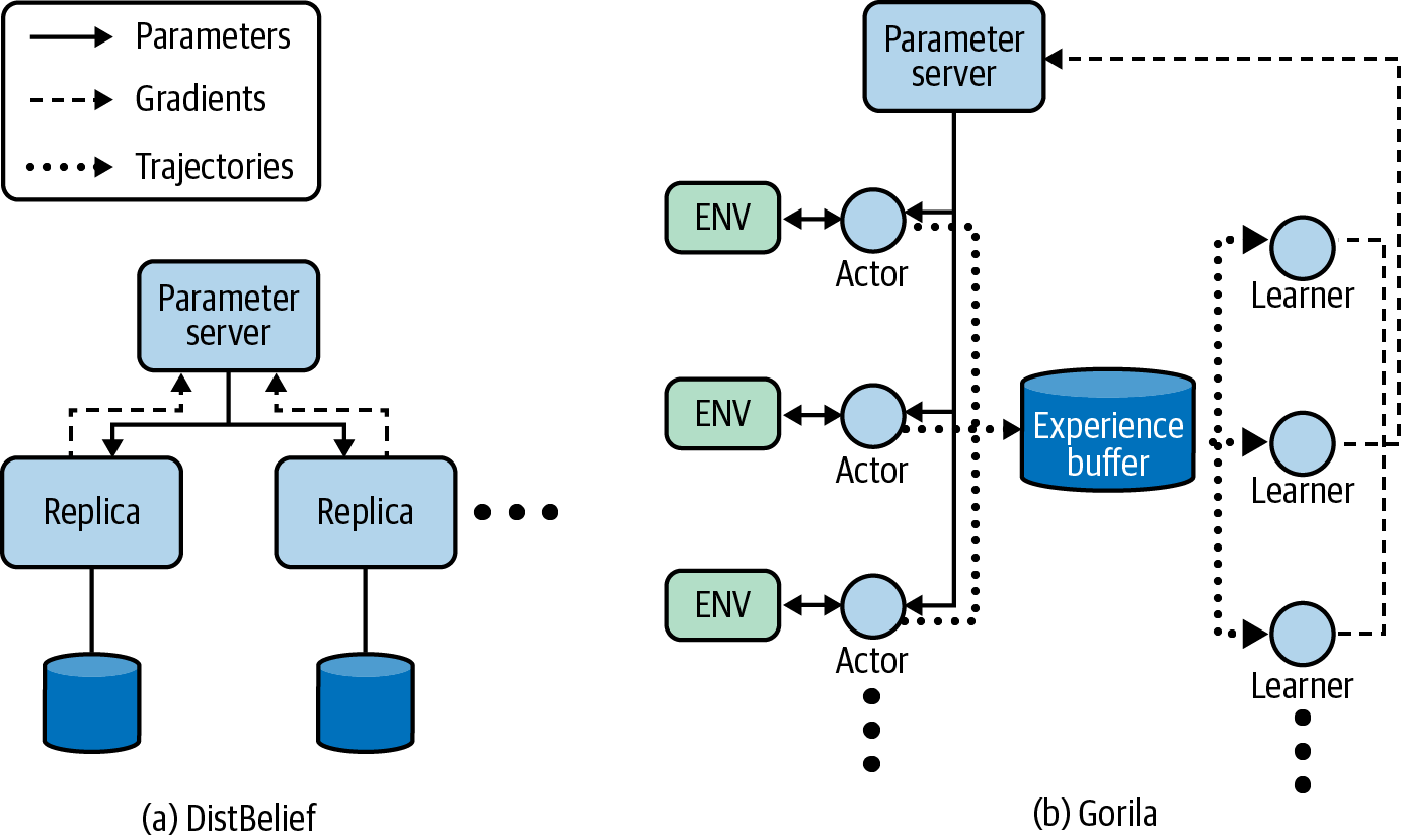
Figure 10-1. A component diagram summarizing the architecture for (a) DistBelief and (b) Gorila. Gorila enables scaling by separating the tasks of acting and learning and then replicating.
Single-machine training (A3C, PAAC)
Using Gorila in the Atari environments led to superior performance over 20 times faster (wall-clock time) than DQN alone, but researchers found that a distributed architecture, although flexible, required fast networks; transferring trajectories and synchronizing parameters started to become a bottleneck. To limit the communication cost and simplify the architecture, researchers demonstrated that parallelizing using a single multicore machine is a viable alternative in an algorithm called asynchronous advantage actor-critic (A3C).8 This is a parallel version of the advantage actor-critic algorithm (A2C). Since updates reside within the same machine, the learners can share memory, which greatly reduces the communication overhead due to speedy RAM read/writes. Interestingly, they don’t use a lock when writing to shared memory across threads, which is typically an incredibly dangerous thing to do, using a technique called Hogwild.9 They find that the updates are sparse and stochastic, so overwrites and contention isn’t a problem. Figure 10-2 shows the differences between A2C and A3C algorithms, which both run on a single machine.
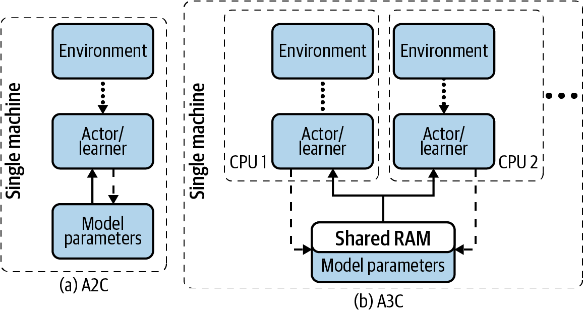
Figure 10-2. A component diagram summarizing the architecture for (a) A2C and (b) A3C. Both algorithms run on a single machine, but A3C uses multiple threads with replicated agents that write to a shared memory.
Surprisingly, using a single machine with 16 CPU cores with no GPU, A3C obtained comparable results to Gorila in one-eighth of the time (1 day) and better results in about half the time (4 days). This clearly demonstrates that synchronization and communication overheads are a big problem.
The simplicity of not using GPUs holds A3C back. It is very likely that a GPU will speed up training of anything “deep,” for greater cost, of course. The parallel advantage actor critic (PAAC) implementation, which isn’t a great name because you can use this architecture with any RL algorithm, brings back the ability to use a GPU. It uses a single learner thread, which is able to use a single attached GPU, and many actors in as many environments. In a sense, this is an intentionally less scalable version of both Gorila and A3C, but it produces comparable results to A3C in one-eighth of the time (again!) creating efficient policies for many Atari games in about 12 hours, depending on the neural network architecture. This implementation shows that increasing exploration through independent environments is a very good way of decreasing the wall-clock training time; training time is proportional to the amount of the state-action space you can explore. Similar to A3C, this implementation demonstrates that data transfer and synchronization is a bottleneck and if your problem allows, you will benefit from keeping the components as close to each other as possible, preferably inside the same physical machine. This is simple, too, in the sense that there are no orchestration or networking concerns. But obviously this architecture might not fit all problems. Figure 10-3 presents this architecture.10
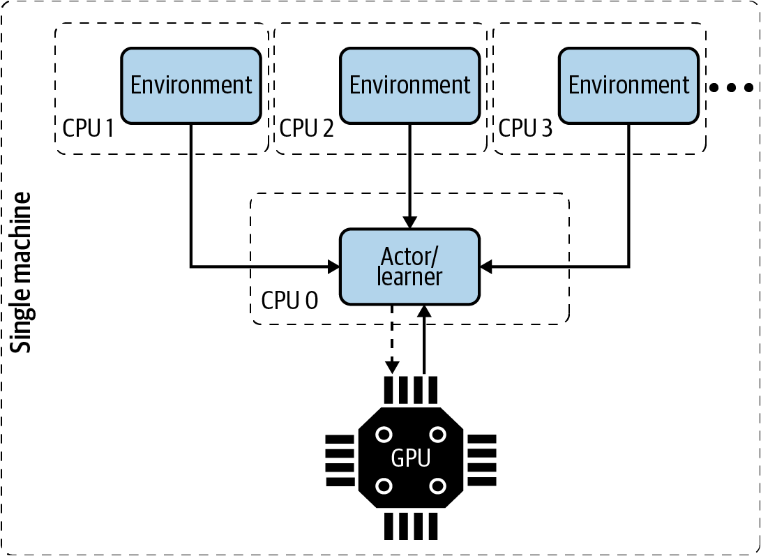
Figure 10-3. A component diagram summarizing the architecture for PAAC. A single machine with a GPU and many CPUs is used to scale the number of environments.
Distributed replay (Ape-X)
Using other types of replay buffer in a distributed setting is as simple as augmenting Gorila’s (or other’s) architecture. Ape-X is one such example, in which greater exploration via distributed actors with environments led to better results, because more diverse experiences were collected. Performance measures on Atari environments were approximately three times greater than AC3 and four times greater than Gorila. But these scores were trained on 16 times the number of CPUs (256 versus 16 for A3C), which led to two orders of magnitude more interaction with the environment. It is unclear whether there was a difference in performance when using the same number of environments/CPUs.11
Synchronous distribution (DD-PPO)
Attempting to use a single machine with many CPUs for training an RL algorithm, like in PAAC or AC3, is enticing due to the simplicity of the architecture. But the lack of GPUs becomes a limiting factor when your problem uses 3D simulators that need GPUs for performance reasons. Similarly, a single parameter server with a single GPU, like in Gorila or PAAC/AC3, becomes a limiting factor when you attempt to train massive deep learning architectures, like ResNet50, for example. These factors call for a distributed architecture that is capable of leveraging multiple GPUs.
The goal of decentralized distributed proximal policy optimization (DD-PPO) is to decentralize learning, much like decentralized, cooperative multi-agent RL. This architecture alternates between collecting experience and optimizing the model and then synchronously communicating with other workers to distribute updates to the model (the gradients). The workers use a distributed parallel gradient update from PyTorch and combine the gradients through a simple aggregation of all other workers. The results show that DD-PPO is able to scale GPU performance by increasing the number of workers almost linearly, tested up to 256 workers/GPUs. The primary issue with this implementation is that the update cannot occur until all agents have collected their batch. To alleviate this blocking, Wijmans et al. implemented a preemptive cutoff, which forces a proportion of stragglers to quit early. Figure 10-4 summarizes this architecture and Wijmans et al. suggest that it is feasible to implement any RL algorithm.12 Other researchers have suggested a similar architecture.13
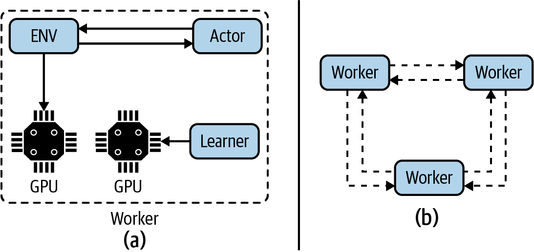
Figure 10-4. A component diagram summarizing the architecture for DD-PPO. A worker (a) comprises an environment, actor, and learner that are able to leverage GPUs. (b) After the agent collects a batch of data each worker performs a distributed update to share weights.
Improving utilization (IMPALA, SEED)
Importance weighted actor-learner architecture (IMPALA) is like a combination of Gorila and DD-PPO. The key advancement is that it uses a queue to remove the need for synchronizing updates. The actor repeatedly rolls out experience and pushes the data into a queue. A separate machine (or cluster of machines) reads off the queue and retrains the model. This means that the update is off-policy; the learner is using data from the past. So IMPALA uses a modified version of the retrace algorithm (see “Retrace()”) to compensate for the lag in policy updates. This also enables the use of a replay buffer, which improves performance.
Espeholt et al. demonstrate that the basic off-policy actor-critic (see “Off-Policy Actor-Critics”) works almost as well, which implies that more sophisticated versions like TD3 might work better. Indeed, OpenAI used an IMPALA-inspired framework with PPO for its Dota 2 video game competition.14
Single learners with multiple actors typically run on a single machine. You can duplicate the architecture to increase the number of learners and use distributed training like DD-PPO. This architecture, depicted in Figure 10-5, improves training speed by an order of magnitude compared to A3C, but is proportional to the amount of hardware in the cluster (they used 8 GPUs in their experiments). Espeholt et al. also claim that this architecture can be scaled to thousands of machines.15
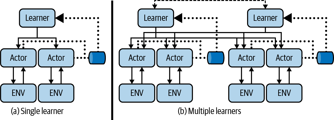
Figure 10-5. A component diagram summarizing the architecture for IMPALA. A single learner (a) has multiple actors (typically on the same machine). Actors fill a queue and training is performed independently of the actors. When using multiple learners (b) gradients are distributed and trained synchronously (like DD-PPO).
Although IMPALA is efficient and is capable of state-of-the-art results, there are still parts of the architecture that can be optimized. One problem is the communicating of the neural network parameters. In large networks these are represented by up to billions of floats, which is a large amount of data to transfer. Observations, on the other hand, are typically much smaller, so it might be more efficient to communicate observations and actions. Also, environments and actors have different requirements, so it could be inefficient to colocate them on the same CPU or GPU. For example, the actor might need a GPU for quick prediction, but the environment only needs a CPU (or vice versa). This means that for much of the time the GPU won’t be utilized.
Scalable and efficient deep RL with accelerated central inference (SEED) aims for an architecture where environments are distributed, but request actions from a central, distributed model. This keeps the model parameters close to the model and allows you to choose hardware that maps directly to either environment simulation or model training and prediction. This leads to increased utilization and slightly faster training times (approximately half the time under similar conditions). Figure 10-6 depicts a simplified version of the architecture.16
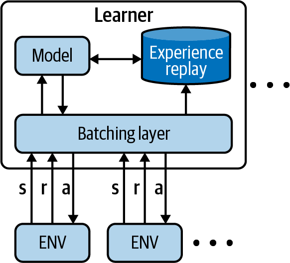
Figure 10-6. A component diagram summarizing the architecture for SEED RL. Hardware is allocated according to the need of the model or environment.
One interesting aspect of the SEED paper is that it highlights how coupled the architecture is to performance. In order to generate their results the researchers had to treat the number of environments per CPU and the number of CPUs as hyperparameters. In general more replicas produced higher scores in less time, but precise configurations are probably environment dependent and therefore hard to pinpoint. Another point to make is that SEED goes to great lengths to optimize on a software level, too, using a binary communication protocol (gRPC) and compiled C++.
Both IMPALA and SEED are capable of running on a single machine, like A3C and PAAC, and are generally more performant due to higher utilization.
Scaling conclusions
The previous algorithms achieve state-of-the-art results in a short period of time. But these comparisons are made on toy environments—the Atari environment, mostly, but sometimes more continuous environments like Google Research Football. You can extrapolate results from these environments to real-life scenarios, but the reality is you are going to have to do your own testing to be sure.
Researchers have a lot of experience with these environments, so they don’t have to waste too much time tuning them and they already know the pitfalls to look out for. But they also aim for headline results, like state-of-the-art performance or speed. There is a hyper-focus on utilization and uber-scale and that sometimes comes at a cost. For example, having a fully distributed deployment like DD-PPO might actually be better for operational use because it would be easy to make it self-healing (just form a cluster of some number of distributed components), which increases robustness and high-availability. This might not be of interest for your application, but my point is that fastest isn’t always best. There are other important aspects, too.
Similarly, you can start to see diminishing returns, too. Early improvements yielded a reduction of an order of magnitude in training speed. The difference between IMPALA and SEED was about half. Researchers are having to go into increasing depth to extract more performance, like statically compiling code and using binary protocols. Again, this may not be appropriate for your problem. If you had to write code in C++ rather than Python, for example, the cost of your time or the opportunity loss may be greater than the gains obtained through code-level optimization.
Finally, some of these architectures tend to blur the abstractions that have emerged in the frameworks. It is common to have abstractions for agents, environments, replay buffers, and the like, but these architectures enforce locations for these abstractions, which might not be ideal from a design perspective. For example, bundling the model, the training, the replay buffer, and some custom batching logic into the learner in the SEED architecture could get messy. It would have been great if they were physically distinct components, like distributed queues and ledgers. Obviously there is nothing stopping you from implementing something like that, but it is generally not a priority for this kind of performance-driven research.
Evaluation
To add value to a product, service, or strategy, you and your stakeholders need to carefully consider what you are trying to achieve. This sounds abstract and high level, but it is too easy to work hard on a problem only to find that the thing that you are optimizing for doesn’t fit the goal. The reason is that engineers can forget, or even ignore, to connect their work back to the objective.
Psychologists and neurologists have studied multitasking at great depth. They found that humans have a limited amount of mental energy to spend on tasks and that switching between several severely impacts performance. But when working on engineering problems, switching between abstraction levels is just as difficult. Your brain has to unload the current stack of thought, save it to short-term memory, load up a new mental model for a different abstraction level, and start the thought process. This switching, along with the effort of maintaining your short-term memory, is mentally taxing. This is one reason why it is easier to ignore high-level objectives when working on low-level day-to-day challenges.
Another reason, even after the dawn of DevOps, is that engineering is deemed to be successful when forward progress is made: new products, new features, better performance, and so on. Moving backward is viewed as a lack of progress; I want to make it clear that it is not. “Going back to the drawing board” is not a sign of failure, it is a sign that you have learned important lessons that you are now exploiting to design a better solution.
Even though it can be hard, try to take time to move around the development process, and up and down through abstraction layers to make sure they are all aligned toward the goal you are trying to achieve.
Tip
Here’s one trick that I use to force myself to switch abstractions or contexts: ask the question “Why?” to move up an abstraction layer and ask the question “How?” to move down.
Coming back to the task at hand, when evaluating your work, you should initially ask why you want to measure performance. Is this to explain results to your stakeholders? Or is it to make it more efficient? Answers to this question will help direct how you want to implement.
Policy performance measures
The efficacy of an RL agent can be described by two abstract metrics: policy performance and learning performance. Policy performance is a measure of how well the policy solves your problem. Ideally, you should use units that map to the problem domain. Learning performance measures how fast you can train an agent to yield an optimal policy.
In a problem with a finite horizon, which means there is a terminating state, the policy performance is most naturally represented by the sum of the reward. This is the classic description of an optimal policy. In infinite-horizon problems you can include discounting to prevent rewards tending to infinity. Discounting is often used in finite problems, too, which might lead to a subtly different policy, so you should consider removing it when you compute the final performance measure. For example, your stakeholders are probably not interested in discounted profit; they want to talk about profit.
Another option is the maximization and measurement of average rewards. In the average-reward model, you have to be careful to ensure that the mean is a suitable summary statistic for your distribution of rewards. For example, if your reward is sparse, then an average reward is a poor summary statistic. Instead, you could choose other summary statistics that are more stable, like the median or some percentile. If your rewards conform to a specific distribution, then you might want to use parameters of that distribution.
Measuring how fast an agent can learn an optimal policy is also an important metric. It defines your feedback cycle time, so if you use an algorithm that can learn quicker you can iterate and improve faster. In problems where agents learn online, for example if you are fine-tuning policies for specific individuals, learning quickly is important to mitigate the cost of missing an opportunity due to suboptimal policies.
The simplest measure of training performance is the amount of time it takes for the agent to reach optimality. Optimality is usually an asymptotic result, however, so the speed of convergence to near-optimality is a better description. You can arbitrarily define what constitutes “near” for your problem, but you should set it according to the amount of noise in your reward score; you may need to perform averaging to reduce the noise.
You can define time in a few different ways, depending on what is important to your problem. For simulations, using the number of steps in the environment is a good temporal measure because it is independent of confounders and environment interactions tend to be expensive. Wall-clock time could be used if you are concerned about feedback cycle time and can limit the number of environment interactions. The number of model training steps is an interesting temporal dimension to analyze model training performance. And computational time can be important if you want to improve the efficiency of an algorithm.
Your choice of temporal dimension depends on what you are trying to achieve. For example, you might initially use environment steps to improve the sample efficiency. Then you might start looking at wall-clock time when you are ready to speed up training. Finally, you might squeeze out any remaining performance by looking at process time. Typically you would use all of these dimensions to gather a broad picture of performance.
Regret is used in online machine learning to measure of the total difference between the reward if an agent was behaving optimally in hindsight and the actual reward obtained over all time. It is a positive value that represents the area between the optimal episodic reward and the actual, as shown in Figure 10-7. Imagine you run a solar power plant. The total amount of power you generate in an episode, which might be one day, has a fixed maximum that is dependent on the amount of sun and the conversion efficiency of the solar panels. But you are training a policy to alter the pitch of the panels to maximize power output. The regret, in this case, would be the difference between the theoretical maximum power output and the result of the actions of your policy summed over a period of time.
Regret has been used by researchers as a mathematical tool during the formulation of policy algorithms, where the policy optimizes to limit the regret. This often takes the form of a regularization term or some adaptation of the rewards to promote statistically efficient exploration (see “Delayed Q-Learning”, for example). Regret is important conceptually, too, since humans reuse experience to infer causation and question the utility of long-term decisions.17

Figure 10-7. A depiction of how to calculate regret while training a policy over time. Regret is the shaded area.
You can use regret as a measurement of performance, too, but how you decide what the optimal policy is, even in hindsight, is dependent on the training circumstances. You might not be able to obtain a theoretically optimal policy or it may not be stationary, for example. If the policies are operating in a nonstationary environment, then approaches include attempting to calculate the regret within a small interval. In simpler problems you might be able to, in hindsight, establish what the best action was and use that as the optimal reward. In more complex problems you should be able to use another algorithm as a baseline and make all comparisons to that. If possible, you could use self-play to record the opponent’s positions and then after the game has finished see if there were better actions you could have played. There isn’t yet a simple unified method of calculating regret for any problem.
Statistical policy comparisons
Whenever you are making comparisons I always recommend that you visualize first. Statistics is full of caveats and assumptions and it’s very easy to think that you are doing the right thing, only to have someone more mathematically inclined say that what you did only makes sense in a very specific circumstances. Visualizing performance is much easier because it is intuitive. You can leverage visual approximations and models that you have learned throughout your life. For example, fitting a linear regression model by eye, even with noise and outliers, is much easier for humans than the mathematics suggest. Similarly, comparing the performance of two algorithms is as simple as plotting two metrics against each other and deciding which is consistently better than the other.
However, there are times when you do need statistical evidence that one algorithm is better than another. If you want to automate the search for a better model, for example, then you don’t want to have to look at thousands of plots. Or if you want a yes/no answer (given caveats!). Here is a list of possible statistical tests with brief notes of their assumptions when comparing two distributions:
- Student’s t-test
- Welch’s t-test
- Wilcoxon Mann-Whitney rank sum test
-
Compares medians, is nonparametric, therefore no assumption on distribution shapes. But does assume they are continuous and have the same shape and spread.
- Ranked t-test
-
Compares medians, are ranked and then fed into t-test. Results are essentially the same as the Wilcoxon Mann-Whitney rank sum test.
- Bootstrap confidence interval test
-
Randomly samples from distributions, measures difference in percentiles, and repeats many times. Requires very large sample size, approximately greater than . No other assumptions.
- Permutation test
-
Randomly samples from distributions, randomly assigns them to hypotheses, and measures the difference in percentiles, and repeats many times. Similar to the bootstrap confidence interval test but instead tests to see if they are the same, to some confidence level. Requires very large sample sizes again.
You can see that there are a lot of varied assumptions, which make it really easy to accidentally use the wrong test. And when you do, they fail silently. The results won’t show you that you have done something wrong. So it’s really important to have strong expectations when performing these tests. If the results don’t make sense, you’ve probably made a mistake.
What are the problems with these statistical assumptions?
-
RL often produces results that are not normal. For example, an agent can get stuck in a maze 1 in 100 times and produce an outlier.
-
Rewards may be truncated. For example, there may be a hard maximum reward that results in discontinuity in the distribution of results.
-
The standard deviations of the runs are not equal between algorithms and may not even be stationary. For example, different algorithms might use different exploration techniques that lead to different variations in results. And within the evaluation of a single algorithm, there may be some fluke occurrence like a bird flying into a robotic arm.
Colas et al. wrote an excellent paper on statistical testing specifically for comparing RL algorithms. They compare the performance of TD3 and SAC on the Half-Cheetah-v2 environment and find that they need to rerun each training at least 15 times to get statistically significant evidence that SAC is better than TD3 (on that environment). They suggest that for this environment, rewards tend to be somewhat normal so Welch’s t-test tends to be the most robust for small numbers of samples. The nonparametric tests have the least assumptions but require large sample sizes to approach the power of assuming a distribution.18 They also have a useful repository that you can leverage in your experiments.
You might be asking, “What does he mean by rerun?” That’s a good question. If you read through enough papers on RL algorithms you will eventually see a common evaluation theme. Researchers repeat an experiment 5 or 10 times then plot the learning curves, where one experiment represents a full retrain of the algorithm on a single environment. Upon each repeat they alter the random seed of the various random number generators.
This sounds simple but I’ve found it to be quite tricky in practice. If you use the same seed on the same algorithm it should, in theory, produce the same results. But often it doesn’t. Usually I find that there is yet another random generator somewhere buried within the codebase that I haven’t set. If you train an algorithm using a typical set of RL libraries then you have to set the seed on the random number generators for Python, Numpy, Gym, your deep learning framework (potentially in several places), in the RL framework, and in any other framework you might be using, like a replay buffer. So first check that you can get exactly the same result on two runs. Then you can repeat the training multiple times with different values for the random seed. This produces a range of performance curves that are (hopefully) normally distributed.
The problem is that researchers tend to use a small, fixed number of repeats because training is expensive. If there is a large separation between the two distributions then a small sample, just enough to be confident of the mean and standard deviation, is adequate. But when the difference in performance is much smaller, you need a much larger sample size to be confident that performance is different. Another paper by Colas et al. suggests that you should run a pilot study to estimate the standard deviation of an algorithm, then use that to estimate the final number of trials required to prove that it outperforms the other algorithm, to a specified significance level.19
Finally, statistical performance measures are one way of quantifying how robust a policy is. The standard deviation of an obtained reward is a good indication of whether your policy will survive the natural drift of observations that occur so often in real life. But I would recommend taking this a step further, actively perturbing states, models, and actions to see how robust the policy really is. Adversarial techniques are useful here, because if you can’t break your model, this makes it less likely that real life will break your model, too—life breaks everything eventually.20
Algorithm performance measures
I would suggest that in most industrial problems you have a single or a small number of problems to target and therefore a small number of environments. However, if you are more involved in pure research or you are trying to adapt your implementation to generalize over different problems, then you should consider more abstract performance measures that explain how well it performs at RL-specific challenges.
One of the most useful solutions so far is the behavior suite by Osband et al. They describe seven fundamental RL challenges: credit assignment, basic (a competency test, like bandit problems), scalability, noise, memory, generalization, and exploration. An agent is tested against a handpicked set of environments that correspond to the challenge. The agent then receives a final aggregated score for each challenge that can be represented in a radar plot, like in Figure 10-8.21

Figure 10-8. Comparing several algorithms using the behavior suite. Each axis represents a different RL challenge. Note how the random agent performs poorly on all challenges and standard DQN performs well on many except for exploration and memory. Used under license, Apache 2.0.
Problem-specific performance measures
There are also a range of benchmarks available for domain-specific tasks, or for tasks that have a particularly tricky problem. For example, there are benchmarks for offline RL, robotics, and safety.22,23,24 Many more excellent benchmarks exist.
These can be useful when you know you also have the same generic problem in your domain and can be confident that improvements in the benchmarks translate to better performance in the real world.
Explainability
An emerging phase in the data science process is explainability, often abbreviated to explainable artificial intelligence (XAI), where you would use techniques to attempt to describe how and why a model made a decision. Some algorithms, like tree-based models, have an inherent ability to provide an explanation whereas others, like standard neural networks, must rely on black-box approaches, where you would probe with known inputs and observe what happens at the output.
Explainability is important for several reasons. One is trust; you shouldn’t put anything into production that you don’t trust. In software engineering this trust is established through tests, but the complexity of models and RL means that the “coverage” is always going to be low. Another reason might be that there is a regulatory or commercial reason to explain decisions like the EU General Data Protection Regulation or Facebook’s post recommendation explanation feature. Being able to explain an action or decision can also help with debugging and development.
Explainability is harder in RL than in machine learning because agents select sequential actions whose effects interact and compound over long periods. Some RL algorithms have an intrinsic capability to explain. Hierarchical RL, for example, decomposes policies into subpolicies, which combine to describe high-level behavior. But most research focuses on black-box, post-training explainability, because it is more generally applicable.
The black-box techniques tend to operate on either a global or local level. Global methods attempt to derive and describe the behavior at all states, whereas local methods can only explain particular decisions.
Global methods tend to consist of training other, simpler models that are inherently explainable, like tree or linear models. For example, the linear model U-trees model uses a tree structure to represent a value function, with linear approximators at the leaf of each tree to improve generalization. From this model you can extract feature importance and indicative actions for all of the state space.25
Local methods comprise two main ideas. The word “local” is usually meant to denote a global method evaluated in a small region of the state space. For example, Yoon et al. use RL to guide the process that trains the local approximation.26 Other ideas expand upon the predictive nature of global methods by considering the counterfactual, the opposite action or what could have happened. Madumal et al. achieve this by training a model to represent a causal graph that approximates the environment transition dynamics. This sounds promising but only works with discrete states.27
Similar to explaining decisions, it can also be useful to indicate what parts of the state influence a decision. For problems with visual observations, or states that have some notion of position or adjacency, you can use saliency maps to highlight regions that are important to action selection.28
Evaluation conclusions
Evaluation is an inherent part of life, from karate belts to food critics. In industrial applications, evaluating your work helps you decide when you are finished. In software engineering, this is usually when acceptance tests have passed. In machine learning acceptable performance is often defined by an evaluation metric. But in RL, because of the strategic nature of the decisions being made, it is very hard to state when enough is enough. You can always make more profit, you can always save more lives.
In general, the performance of an agent is defined by the reward obtained by the policy and how fast it got there. But there are a range of other measures that you should also consider if you want to train and utilize a stable, robust policy in a production situation. This also includes the ability to explain the decisions of a policy, which could be vitally important in high-impact applications.
Deployment
By deployment, I refer to the phase where you are productionizing or operationalizing your application. Projects come to a point where everyone agrees that they are both viable and valuable, but to continue being viable and valuable they need to be reliable. This section is about how to take your budding RL proof of concept into the big league so that you can serve real users.
The tricky part is that there isn’t much prior work on running RL (RL) applications operationally. So much of this has to be extrapolated from running software and machine learning applications, my experience running Winder Research, and the many luminaries who have penned their own experiences.
Goals
Before I dig into the details of deployment, I think it is important to consider the goals of this phase of the process. This will help you focus on your situation and help you decide what is important to you, because no one idea or architecture is going to suit all situations.
Goals during different phases of development
First, consider how the deployment priorities change depending on what phase of development you are in. There are three phases where you need to be able to deploy an agent: during development, hardening, and production.
During development it is important to have an architecture that allows you to rapidly test new ideas; flexibility and speed trumps all other needs. This is because during early phases of a project it is important to prove the potential viability and value. It is not important to be infinitely scalable or exactly repeatable; that comes later. The largest gains come from rapid and diverse experimentation, so the largest cost at this point in time is the length of that feedback loop.
Once a project has proven to be viable and valuable, then it goes through a phase of hardening. This involves improving the robustness of the processes involved in maintaining a policy. For example, offline policies or ancillary models must be trained, which may require large amounts of computational resource, and the provenance (the origin of) of a codebase or model is vital to ensure you know what will be running in production.
Finally, policies and models are deployed to production and used by real people or processes. Because RL optimizes sequences of actions, it is highly unlikely that you will be able to retrain your policy by batching data once every so often, which is the predominant technique used in production machine learning systems, so care must be taken to preserve the state of the policy. This phase encourages the development and adoption of sophisticated monitoring and feedback mechanisms, because it is so easy for the policy to diverge (or at least not converge).
When deploying an RL solution into a product or service, the value of performing a task changes. Early on, the quickest way to extract value is through rapid experimentation and research; later on reliability, performance, and robustness become more important. This leads to a range of best practices that are important at different times.
Best practices
Machine learning operations (MLOps) is an emerging description of the best practices and appropriate tooling that is required to run production-quality models. The need for this has arisen because machine learning models have different operational requirements compared to traditional software projects, but fundamentally the core needs are exactly the same. I like to summarize these needs into three topics: reliability, scalability, and flexibility.
Reliability lies at the core of modern software engineering. Thousands of books have been written on the topic and these ideas are directly applicable to machine learning and RL, ideas like testing, continuous integration and delivery, architecture, and design. Moving toward machine learning, ideas such as building data pipelines, provenance, and repeatability all aim to solidify and further guarantee that models will continue to work into the future. RL poses its own challenges and over time I expect new best practices to emerge.
For example, I caught up with an old colleague recently and I was asking about some previous projects that we collaborated on. I had developed some algorithms to perform traffic and congestion monitoring around 2012 and these had been deployed to some major roads in the UK on dedicated hardware. I learned that the hardware had failed twice but my algorithms (in Java!) were still going strong, nearly 10 years later. This fact isn’t due to my algorithms, it is due to my colleagues’ software engineering expertise and a commitment to reliable software.
Scalability is particularly important to both machine learning and RL, arguably more so than typical software, because they need so much horsepower to do their job. If you consider all software ever written, the vast majority of those applications will probably run on the resources provided by a standard laptop. Only rarely do you need to build something that is as scalable as a global messaging or banking system. But in machine learning and RL, nearly every single product ever produced needs far more than what a laptop can provide. I posit that the average computational requirement for an RL product is several orders of magnitude greater than a software product. I am being intentionally vague, because I don’t have any hard facts to support this. But I think my hypothesis is sound and this is why scalability is an important factor when deploying RL.
I think flexibility is one of the most underrated best practices. In industry, reliable software was the theme of the first decade in the 21st century, with software architecture, test-driven development, and continuous integration being hot topics at conferences around the world. In the second decade, scalability was the golden child and resulted in important changes like cloud adoption and the subsequent need for orchestration. I think the third decade (I’m ignoring specific themes like artificial intelligence and RL and machine learning) will focus on flexibility, purely because I see industry trending toward hyper-responsibility, where the most valuable engineers are defined by their ability to fulfill all of the roles expected in an enterprise environment, from business development through to operations. The field of DevOps can only ever expand; it can never shrink back to two separate roles.
A similar argument can be made about the pace of change today. Engineers are continuously creating new technologies and it’s hard to predict which will withstand the test of time. But I find that when tools attempt to enforce a fixed, inflexible, or proprietary way of working, they quickly become cumbersome to work with and are quickly outdated. No, flexibility is the only way to future-proof systems, processes, and solutions.
Hierarchy of needs
Maslow’s hierarchy of needs was an early psychological model suggesting human necessities depicted as a hierarchical model; in order to have safety you need access to air and water, in order to have friendship you need to be safe, and so on. RL has a similar hierarchy of needs.
To have a viable RL problem then you need an environment in which you can observe, act, and receive a reward. You need the computational ability to be able to decide upon actions given an observation. These things are required and if you don’t have them, then you can’t do RL.
Above that comes things that are valuable, but not strictly necessary. For example, pipelines to transform data in a unified, reliable way will prevent data errors. Being able to specify exactly what is running in production—provenance—is operationally useful.
The layer above this represents an optimal state, one that is probably more conceptual than practical in many cases, because tackling other problems or developing new features might be more valuable in the short term. Here you might consider fully automating the end-to-end process of whatever it is you are doing, or incorporating a sophisticated feedback mechanism to allow your product to automatically improve itself.
Table 10-1 presents some example implementation and deployment challenges that you might face. I want to stress that these have a range of solutions with variations in the amount of automation. But the value of each level of automation depends on your or your stakeholder’s assessment of other pressing needs. Just because there is a more sophisticated solution that doesn’t mean what you have isn’t good enough already. Get the basics right first.
| Infrastructure | State representation | Environment | Learning | Algorithm improvement | |
|---|---|---|---|---|---|
Optimal |
Self-healing |
Continuously learning |
Combination |
Meta |
Automated |
Valuable |
Automated deployment |
Model-driven dimensionality reduction |
Real life |
Offline |
Brute-force selection |
Required |
Manual deployment |
Fixed mapping |
Simulation |
Online |
Manual |
Architecture
There hasn’t been a huge amount of research into generic RL architectures and I can think of a few reasons to explain this. The first is that RL still isn’t universally accepted as a useful tool for industrial problems, yet. Hopefully this book will start to change that. This means that there isn’t enough combined experience of designing these kinds of systems and therefore it has not been disseminated to a wider audience. Secondly, researchers, especially academic researchers, tend to be more focused on groundbreaking research, so you will find few papers on the subject. Third, I don’t think there is a one-size-fits-all approach. Compare the differences between single-agent and multi-agent RL, for example. And finally, the deployment architecture is mostly a software engineering concern. Of course there are RL-specific needs, but I think that typical software architecture best practices fit well.
With that said, there is some literature available from the domain of contextual bandits. It’s not generally applicable, but because industry has been quicker to adopt this technique, many lessons have already been learned. Two of the biggest problems that lead to architectural impacts are the fact that agents can only observe partial feedback and that rewards are often delayed or at worst, sparse:29
-
Machine learning is considered to be simpler, because feedback, or ground truth, is complete. The label represents the single correct answer (or answers if multiple are correct). RL only observes the result of a single action; nothing is learned from the unexplored actions (which are possibly infinite).
-
Rewards observed by the agent are often delayed, where the delay ranges from millisecond scales in bidding contests to days when people are involved. Even then, the reward may be sparse because the sequence of actions doesn’t lead to a real reward for some time, like a purchase.
Some problems have a relationship with prior work in machine learning, but are accentuated by RL. For example, online learning, or continuous learning, is important in some machine learning disciplines, but RL takes this to a whole new level, since decisions have wide reaching consequences and policies are nonstationary. Even if you are incorporating batch RL, it is important to have a low-latency learning loop. Reproducibility becomes a big problem, too, since both the policy and the environment are constantly shifting.
All of these facets lead to the following range of architectural abstractions that might be useful in your problem:
- Serving interface
-
Like a personalized shopping assistant, one abstraction should contain the ability to serve action suggestions and embed exploration. This should implement the Markov decision process interface and communicate with the wider system or environment. This is the both the entry and exit point of the system and presents a great location to decouple RL from wider deployments.
- Log
-
Like in a message bus queue, it is vitally important to be able to retain state, for several reasons. First is for disaster recovery; you may need to replay interactions to update a policy to the last known state. The second is that it can be used as part of a wider batch or transfer learning effort to improve models. And third, it acts as a queue to buffer potentially slow online updates.
- Parameter server
-
A place for storing the parameters of a model, like a database, crops up in multi-agent RL, but it is useful for situations where you need to replicate single-agent policies, too, to handle a larger load.
- Policy servers
-
Since RL algorithms tend to be customized for a particular problem it makes sense to have an abstraction that encapsulates the implementation. In simpler, more static problems you might be able to bake the parameters of the model into the encapsulation, otherwise you can leverage a parameter server. You can replicate the policy servers to increase capacity.
- Replay buffers
-
Many algorithms leverage replay buffers to increase sample efficiency. This might be an augmentation of the log or a dedicated database.
- Actors and critics
-
You might want to consider splitting the policy server into smaller components.
- Learning
-
Ideally you should use the same policy code to learn or train as you do to serve. This guarantees that there is no divergence between training and serving.
- Data augmentation
-
You might have parts of your algorithm that rely on augmented data; a state representation algorithm, for example. These should exist as traditionally served ML models with their associated continuous integration and learning pipelines.
All or none of these abstractions might appear in your architecture design. Unfortunately they are very domain and application specific, so it doesn’t make sense to enforce these abstractions. Also, more abstractions generally increase the maintenance burden; it’s easier to work from a single codebase, after all. Instead, provide the tools and technologies to enable these architectural capabilities on a per-application basis.
Ancillary Tooling
I’m hesitant to talk about tooling in detail, because of the fast-pace change in the industry; a component I describe here could be obsolete by the time this book goes to print. Instead, I will talk abstractly about the functionality of groups of tooling and provide a few (historical) examples. Refer back to “RL frameworks” for a discussion specific to RL tooling.
Build versus buy
I think the traditional build versus buy recommendations are true in RL, too. If the tool of interest represents a core competency or value proposition then you should build, so that you retain the intellectual property, have much greater depth, and have full control over the customization. Another way of thinking about this is to ask yourself: what are your customers paying you to do?
But if this particular tool does not represent your core competency or if it does not provide a competitive differentiation, then you should consider buying or using off-the-shelf components. A middle ground also exists, where you can leverage an open source project to get you to 80% complete and adapt it or bolt on components to get you the rest of the way.
Monitoring
When your product reaches production, you should invest in monitoring. This, singlehandedly, gives you advance warning of issues that affect trust in an algorithm. And trust is important, because unlike traditional software that simply stops working, machine learning and RL are scrutinized like a racing driver critiques the way their car handles. If users receive an odd or unexpected result, this can knock their confidence. Sometimes it’s better to simulate a broken product than it is to serve a bad prediction or recommendation.
I was speaking to a technical lead for a games company once and he said that users react negatively if they play against an automated agent that doesn’t conform to their social norms. For example, if the agent were to take advantage of an opportunity in the game that left the user weak, the user would consider that bad sportsmanship and stop playing the game. And often they had to de-tune their agents to intentionally make bad choices to make the user feel like they had a fighting chance. RL can help in this regard, to optimize for what is important, like user retention, rather than raw performance.
“Evaluation” talked about a range of RL-specific performance measures that you could implement in a monitoring solution. This is in addition to all the standard machine learning statistics you might monitor and low-level statistical indicators of the underlying data. Of course, software-level monitoring is vitally important. This forms a hierarchy of metrics that you should consider implementing to gain operational insight and spot issues before your users do.
Logging and tracing
A log is an important debugging tool. It tends to be most important during development, to help you tune and debug your agents, and after a failure, to perform a post-mortem analysis. Bugs in traditional software appear when the state of the program changes in a way that is unexpected. So logging these state changes is a good way of tracking down issues when they do occur. But in RL, every interaction with an agent is a state change, so this can quickly become an overwhelming amount of information. This is why I recommend having a dedicated log for Markov state changes, to free your software of this burden.
One of the most common bugs in RL is due to differences in the runtime and expected shape of data. It is a good idea to log these shapes, maybe in a low-level debug log, so you can quickly find where the discrepencies are when they happen. Some people go to the extent of making these assertions to halt the code as soon as an exception is found. The next most common arise from the data, but I wouldn’t save data directly to a text-based log. It’s too much data. Summarize it and save it as a metric in the monitoring or dump it to a dedicated directory of offline inspection.
Tracing decisions through a log can be quite tricky because of the potential length of trajectories. A bad recommendation might not have been caused by the previous action. An action a long time ago could have led to this bad state. This problem is very much like the tracing systems used in microservice deployments to track activity across service boundaries. These systems use a correlation identifier (a unique key) that is passed around all calls; this key is used to link activity. A similar approach could be used to associate trajectories.
There can be other sources of state change, too: changes in the policy, user feedback, or changes in the infrastructure, for example. Try to capture all of these to be able to paint a picture when things go wrong. If you do have failures and you don’t know why, be sure to add appropriate logging.
Continuous integration and continuous delivery
Continuous integration is a standard software engineering practice of building automated pipelines to deploy your solutions. The pipelines perform tests to maintain the quality of your product. Continuous delivery is the idea that if you have enough confidence in your quality gates, then you can release a new version of your software upon every commit.
CI/CD is an important and necessary tool for production deployments, but it only operates on offline, static artifacts like software bundles. It can’t provide any guarantees that the data flowing into, through, or out of your agent is valid.
You can tackle the internal part with testing. You can monitor and alert upon the data flowing out. But even though you could monitor the data flowing in, it might still cause a catastrophic failure.
To handle problems with incoming data you need to test it. I call this “unit testing for data.” The idea is that you specify what you expect incoming data to look like in the form of a schema and test that it conforms. If it doesn’t you can either correct it or inform the user there was something wrong with their data. You have to make an architectural decision about where to perform this testing. The simplest place is in the serving agent, but this could bloat the code. You could have a centralized sentry that manages this process, too.
Experiment tracking
During development you will be performing a large number of experiments. Even after this phase, you need to keep track and monitor the performance of your agent or model as you gather new observations. The only way to do this consistently is to track performance metrics.
The underlying goals are similar to monitoring: to maintain quality and improve performance. But monitoring only provides information about the current instantiation of the agent. Experiment tracking intends to provide a longer-term holistic view, with an eye on potential improvements.
The idea is that for every run of an agent, you should log and track the performance. Over time you will begin to see trends in the performance of agents as the data evolves. And you can compare and contrast that to other experiments.
But the main reason why it is important is that training can sometimes take days, so to maintain efficiency you have to run experiments in parallel. For example, imagine you had designed a recommendations agent and had a hypothesis that it was easier to learn policies for older people, because they knew what they wanted. So you segmented the training data by age and started training upon several different datasets. Instead of waiting for each one to finish, you should run all experiments in parallel, and track their results. Yes, your efficiency is down because of the time it takes to get feedback on your hypothesis, but at least you’ll get all the results at the same time. For this reason, you should track these experiments with an external system so that you can spend the time effectively elsewhere—or take the day off, it’s your call.
In effect, you want to track the metrics, the things you are monitoring, and store them in a database. TensorBoard is one common solution and works well for simple experimentation, but it doesn’t scale very well. Even for individuals it can get hard to organize different experiments. It gets even worse when multiple individuals use the same instance. Proprietary systems are available, but many of them are catered toward traditional machine learning, not RL, and because they are proprietary they are hard to improve or augment.
Hyperparameter tuning
The premise of hyperparameter tuning is quite simple: pick values for the hyperparameters, train and evaluate your agent, then repeat for different hyperparameter values. Once again the main problem is the amount of time it takes to do this by brute force, where you exhaustively test each permutation, because of the time it takes to perform a single run.
It is likely that the insight you can provide into your problem will lead to a carefully selected subset of parameters for which brute force might be enough. But there are newer approaches that attempt to build a model of performance versus the hyperparameter values to iterate toward an optimal model faster. They can also cut training runs short if they see that the final performance is going to be suboptimal. I’ve used Optuna for this purpose and it works well when your hyperparameters are continuous and the performance measure is robust. You can run into problems like when hyperparameters slow down learning and the framework thinks the result is suboptimal, but it might lead to better performance in the long run.
Having a good infrastructure setup that autoscales is important to reduce the amount of time it takes to perform hyperparameter experiments.
Deploying multiple agents
The microservice architectural pattern suits machine learning and RL well. Running multiple agents in production is easier than it was because of advancements in tooling that allow you to create advanced deployments. Here is a list of possible deployment strategies:
- Canary
-
Route a certain proportion of users to a new agent, altered over time. Make sure you have the ability to provide stickiness so that the user’s trajectory is dictated by the same agent. This is usually implemented using the same ideas as tracing.
- Shadowing
-
Running other agents hidden in the background, on real data, but not serving the results to users. This can be tricky to validate, because the hidden agent is not allowed to explore.
- A/B testing and RL
-
Yes, you can use bandits or RL to optimally pick your RL agents. Again, ensure stickiness.30
- Ensembles
-
This is more likely to fall under the banner of algorithmic development, but it is possible to use an ensemble of RL agents to make a decision.31 The theory suggests that the resulting action should be more robust, if agents are diverse.
Deploying policies
There is significant risk involved in deploying a new policy, because it is hard to guarantee that it will not become suboptimal or diverge when learning online. Monitoring and alerting helps, but another way of viewing this problem is in terms of deployment efficiency.
In a way that is similar to measuring sample efficiency, you can count how many times the policy needs to be updated to become optimal, during training. Policies that need to be updated less often are likely to be more robust in production. Matsushima et al. investigate this in their work and propose that policies update only when the divergence between the trajectories of the current and prospective policies become large. This limits the frequency of policy updates and therefore mitigates some of the deployment risk.32
Considering when you want to update your policy is an interesting exercise. You will find that your agent sits somewhere on a continuum that ranges from continuous learning (updating on every interaction) through to batch learning (updating on a schedule) and ending at never updating, as shown in Figure 10-9. There is no right answer, as it depends on your problem. But I recommend that you stay as close to never updating your policy as possible, since this limits the frequency at which you have to monitor your deployment for errors or divergence.33
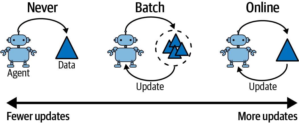
Figure 10-9. How often you update your production policy affects your deployment strategy. It falls on a continuum between never updating (manual deployment) and fully online.
I recommend that you try to make the deployments stateless and immutable, if possible. If you update the parameters of the model this is called a side effect of calling a function. These are considered to be bad because side effects can lead to unexpected failures and make it hard to recover from disaster. For example, one way to achieve immutability is by endeavoring to treat policy updates as new deployments and validating them in the same way you would for a code change. This is extreme, but very robust.
The traditional deployment techniques from “Deploying multiple agents” can also help limit user-facing problems by treating each new instantiation of a policy, as defined by the policy parameters, as a separate deployment. Automated A/B testing can ensure that the new parameters do not adversely affect users.
Safety, Security, and Ethics
RL agents can sometimes control hazardous equipment, like robots or cars, which increases the jeopardy of making incorrect choices. A subfield called safe RL attempts to deal with this risk. RL agents are also at risk from attack, like any connected system. But RL adds a few new attack vectors over and above traditional software and machine learning exploits. And I think that engineers are the first line of defense against ethical concerns and that they should be considered proactively, so I think it’s important to talk about it here.
Safe RL
The goal of safe RL is to learn a policy that maximizes rewards while operating within predefined safety constraints. These constraints may or may not exist during training and operation. The problem with this definition is that it includes ideas about preventing catastrophic updates, in the reward sense. Algorithms have been designed to solve this problem intrinsically, like trust region methods (see “Trust Region Methods”), for example. Another form of research involves extrinsic methods that prevent certain actions from causing physical harm, monetary loss, or any other behavior that leads to damaging outcomes and it is this that I will summarize here. The obvious place to start is with techniques that have already been described in this book.34
If your problem has safety concerns that can be naturally described as a constraint, then you can use any algorithm that performs constrained optimization. TRPO and PPO are good choices, where you can adapt the optimization function to incorporate your problem’s constraints. For example, if you are training an algorithm to deploy replicas of a web service to meet demand, it shouldn’t deploy more than the available capacity of the infrastructure. This information could be provided as a constraint to the optimization function. Ha et al. present a good example of training a robot to prevent falling over using a constrained version of SAC.35
Similarly, you could shape the reward to penalize certain behaviors. For example, a robotic arm will undergo significant stress when fully extended. To prolong the life of the robot you should prevent extensions that might cause metal fatigue. You could incorporate an element that penalizes extension into the reward function.
The problem with these two approaches is that they are hardcoded and likely to be suboptimal in more complex problems. A better approach could be to use imitation or inverse RL to learn optimal constrained actions from an expert.
However, all of the previous approaches do not guarantee safety, especially during learning. Safety is only approximately guaranteed after a sufficient amount of training. Fundamentally, these approaches learn how to act safely by performing unsafe acts, like a child—or an adult—touching a hot cup, despite telling them that the cup is hot.
A more recent set of approaches use an external definition of safety by defining a super-level safe set of states. For example, you could define a maximum range in which a robot is allowed to operate or the minimum allowable distance between vehicles in a follow-that-car algorithm. Given this definition, an external filter can evaluate whether actions are safe or not and prevent them.
A crude filter could prevent the action entirely and penalize the agent for taking an action, which is basically the same as reward shaping, except you prevent the dangerous action taking place. But that doesn’t incorporate the knowledge of the safe set into the optimization process. With this approach, for example, you would have to jump out of a tree at every height before you know for sure that certain actions are unsafe—may I suggest a safety rope.
A more pragmatic approach is to build models that are able to abort and safely reset agents. You can often design your training to avoid unsafe actions by definition. For example, Eysenbach et al. built a legged robot and trained it to walk by changing the goal to be far away from unsafe states. For example, if it moves too far to the left, then the goal is changed to be on the right. They also learn a reset controller to provide an automated method to get back to a safe state.36
Researchers have looked at a variety of ways to incorporate this information. One suggestion is to use rollouts to predict the probability of an unsafe event and prefer actions that lead to safe trajectories.37 This can be incorporated into value-based RL algorithms by pushing the value approximation parameters toward safe states and into policy gradient methods by directing the gradient steps toward safe states, with a correction that accounts for the biased policy generation.38
Another set of suggestions called formally constrained RL attempt to mathematically define and therefore guarantee safety, but these methods tend to rely on perfect, symbolic representations of unsafe states that are only possible in toy examples. One practical implementation from Hunt et al. resorts to using a model-driven action filtering technique.39 Without doubt, this remains an open problem and I anticipate many more improvements to come.
Secure RL
If an attacker could alter the source code of an application they could inject malicious code. This is called a white box attack. Software deployments mitigate this risk with strict access control mechanisms on the codebase. But if the developer exposes the software to the public internet, then they run the risk that the attacker might be able to probe and find a weakness that allows them to alter the running of the application. This external approach is called a black box attack.
Machine learning, or any data-driven process, is also vulnerable to attack. These are broadly classified as attacks targeting either the training phase or the prediction phase. In the training phase, the attacker may be able to alter or manipulate the training data so that the attacker can exploit this data to produce a known result. This is commonly known as poisoning. For example, if an attacker could introduce a spam email with an incorrect label into a public spam dataset then the attacker might be able to reuse a similar email to sell pills that apparently enhance your libido, which would be classified as not spam by any model trained upon that data. Prediction attacks provide or augment the input data to produce invalid results. Many methods are white hat techniques and assume knowledge of the underlying model.40 But more recently researchers have found black box techniques, like where the attacker can create a second model, similar to the first. Once trained, the attacker can generate white hat attacks for the second model and use them to attack the first. This approach shows that attacks are transferable.41 Together, these are known as adversarial attacks.
RL agents can also be attacked, in all the same ways. Your first step should be to fix the basics. An attacker is not going to go to the trouble of creating a trained replica if they can find an open SSH port on one of your servers or someone’s GitHub credentials have been phished and you don’t have multifactor authentication enabled. Next, make sure you have robust data integrity testing and monitoring in place; use rate limiting and denial-of-service protection to limit how much of the model a black-box attacker can explore. Ensure your models are simple and robust, as much as practicable. Consider a research spike to investigate how you could improve the countermeasures put in place for your ML models.
RL poses greater risks because of the increased attack surface. ML models generally have a single entry point, the input, and a single response, the output. In RL, attackers could target the environment, the observation of the environment, the rewards, or the actions. Successfully altering any of these could cause the policy to tend toward a different result. If the attacker has access to internal systems then they could also target ancillary services like the experience replay buffer or the parameter server.
Ways to prevent or mitigate these types of attacks are under active research. One branch reminds us that model robustness is at the heart of a security strategy and is strongly related to safe RL. If you have a model or a policy that works well under adverse conditions then it is less likely to succumb to an external attack. Behzadan and Munir suggest perturbing agents during training to teach them to be more robust to prediction attacks, which is a common strategy to harden ML models.42
Another approach proposed by Liu et al. is to try to detect an adversarial attack and stop it before it does any damage. RL is sequential and often correlated over time, so you could build a model to predict the next state given the current observation. If you calculate the divergence between the prediction and what actually happened, then compare that to “normal” behavior (a model of the typical distribution of divergences), you could build an algorithm to warn you when large divergences are observed.43
You could consider guiding exploration by directing agents’ actions to states that would cause maximum adversarial gain.44 Or even mitigate adversarial training examples by considering the problem to be hierarchical; adversarial poisoning is likely to “look” very different from normal interaction, so hierarchical RL should be able to consider this a subpolicy. The subpolicies could then be analyzed to ensure legitimacy and that the poisoned data is removed.45
As you can see there are many ideas to tackle the many potential attack vectors. But therein lies the problem: potential. Investing time, energy, and money into mitigating these attacks has to be weighed against the probability of them occurring in the first place. For example, if you have an agent that runs on an internal network and is never exposed to the public internet, then I would consider this level of mitigation to be a poor use of time, given the probability of attack being so low. This is why you have to perform a risk analysis for your particular situation.
Attack mitigation also has diminishing returns, because the knowledge and resources to perform an attack increases exponentially. According to Symantec’s 2019 Internet Security Threat Report, a whopping 65% of all targeted hacks were caused by phishing, 23% by unpatched software, and 5% by bogus software updates. Only when you get to the bottom do you find exploits that directly relate to an exposed RL agent: 2% web server exploits and 1% data storage exploits. These statistics demonstrate that basic security practices are more valuable to a company than RL or possibly even ML attack mitigation techniques. To be clear, I’m not suggesting that RL security is unimportant, just get the basics right first.46
Ethical RL
It’s probably not quite the dictionary definition of the term, but I like to think of ethics as a professional consensus of individual morality. This is an important distinction, because what you believe is right and wrong is not necessarily what I believe. But I would like to think that there is a compromise that we can both accept. So morals represent a distribution of beliefs and the mean represents the ethical standards. Engineers, in general, don’t have a single unified way or place to define the ethical means, so it is important that you are aware that they exist, on a conceptual level at least, and that your perspective is but one of many.
I say this not to preach philosophy or religion, but to remind you that you are in a position of power. You have the power and the authority to not only automate decisions (machine learning) but also entire strategies (RL). Whenever you enact these techniques, you are effectively removing the opportunity for a human to make decisions. This could be a good thing, if the decision is trivial or burdensome, but sometimes it is not. Sometimes the decision is so important that it has to be made by a human, so that they can take responsibility for that decision, right or wrong. They are free to use the information provided by an algorithm, but this does not remove that responsibility. Other times the decision might not be so important on a global scale, but it might be important on a human scale; a person may feel a sense of loss or disempowerment if they lose the ability to make a decision.
Unfortunately, the stakeholders (both users and owners) of your systems are generally not able or not in a position to independently assess impact. They may lack the authority or opportunity to protest or they are prevented from understanding the technical intricacies. You are in a position to prevent this from happening. You can explain, in simple terms, what the pros and cons of your solution are in a way that relates to them personally. You can listen to their questions and address their concerns. You can explain when your system works and when it doesn’t and all the assumptions that you have made along the way.
As for you, you are probably lucky enough to be able to choose what work you do, or at least actively decide not to work on something or for someone that violates your moral principles. This is an unspoken benefit of opportunity, education, and engineering. The fact that you are in a position to read this book is a truly remarkable achievement. You can repay this debt by actively considering what is important to you and how your work affects the world. The following is a list of items that may or may not be important to you. Whenever you are developing an application, ask yourself:
- Bias
-
Does this solution affect certain groups of people more than others? Are there aspects of your data that could accidentally add bias?
- Personal impact
-
How does this affect individuals? What will they feel like when they see/use your solution? If people will be impacted, is there a way to mitigate this? Can you include humans in the decision loop?
- Climate
-
How does your solution affect the climate? Is the application valuable enough to be worth the cost in energy?
- Unintended use
-
How else could your application be used? Would you be uncomfortable if it was used in certain industries? Can you prevent that from happening?
- Nefarious use
-
Is your solution, directly or indirectly, going to be used for an activity that you do not agree with?
- Legality
-
Is it legal? Could it be deemed illegal in certain juristrictions or countries?
- Human rights
-
Could your solution violate legal or your definition of human rights? For example, could it affect the privacy of individuals?
- Justification and explainability
-
How can you justify the actions of your algorithm? How much explanation do they need to provide to be deemed trustworthy?
- Performance misinformation
-
Have you explained effects of your algorithm or potential performance in the clearest, most independent way possible? Is there a chance that others could misinterpret your results and be unduly penalized?
On a technical front, there are efforts to attempt to incorporate some of these ideas into machine learning and RL directly. For example, ML-fairness-gym is a set of components that build simple simulations that assess the long-term impacts of decision systems in social environments. For example, in countries around the world credit scores are used to rate how likely individuals are to repay debt. But the fact that companies use this measure encourages individuals to artificially inflate their credit scores through techniques such as credit utilization and even overstating affordability measures on applications. In turn, this makes it harder for people who don’t engage in these tactics, those who don’t have the capability or opportunity to access such information, to access credit when they need it.47
The long-term consequences are so hard to predict that you might consider not doing it at all. But wait, you have access to a framework that is able to monitor and optimize for long-term sequential rewards. Yes, RL. Researchers have gone so far as to suggest that you can use RL to optimize and make ethical decisions, and even consider using reward shaping as a proxy for ethics shaping.48,49 Maybe RL will save the world?
Summary
To the best of my knowledge, this chapter is the first to provide cohesive and comprehensive advice on how to implement and deploy RL agents. There are many tidbits scattered throughout the research papers, but engineers, on average, have simply not had enough experience with RL in production. My hope is that this chapter, and indeed this book, will begin to change that.
Of course this also means that I am writing from the perspective of my experience and what I think is important. Feel free to take this advice and adapt, change, or totally ignore it as you see fit. The sheer breadth of applications means that the circumstances of a project should dictate how these ideas can be applied and the value of doing so.
Despite the lack of production use (compared to machine learning, for example), there are already a wide range of frameworks to help you get started quickly. These range from algorithmic through to operational frameworks and also include specialized ancillary frameworks to implement a specific part of the RL problem. But it is likely, especially if going into production, that you will still need a lot of custom code, since RL is still young. Scaling RL is similarly supported on the training side by frameworks, and traditional software stacks and orchestrators should help you scale into production.
Evaluating agents is crucial, and could have been included in Chapter 9. But I left it to here since it only really becomes crucial when you are looking to deploy your first agent. While you’re in the proof-of-concept phase, you can usually get away with ad hoc evaluation with standard metrics and environment-specific debugging.
When you do find yourself wanting to deploy a project into a setting where other people can use it, you should take a step back and consider the operational aspects of running RL. Take the time to consider what you are trying to achieve and build an architecture that supports those goals. Don’t be afraid to say that certain aspects are not important to save time, but do so only when considering the risks. To support the deployment you will need to leverage a wide range of software engineering and machine learning tooling. Take advantage of these and adapt them to your RL process.
Safe RL is an important topic for agents that interact with the real world and can directly affect algorithm implementations. Try to catch this requirement as early as you can, since popular algorithms may appear to work well, but could be unsafe. Securing your application is important here as it is in any project and there are RL-specific attack vectors to be aware of. But basic security practices should take priority, since these are the focus of most attacks.
And finally, consider how your application impacts ethical concerns, from an industry perspective, and moral concerns, from a personal perspective. This becomes more important and harder to do the higher you go in the decision stack. Ethical machine learning is hard enough to get right, but since RL is automating whole strategies, there is potential for long-term and wide-reaching consequences.
Further Reading
-
-
Martin, Robert C. 2008. Clean Code: A Handbook of Agile Software Craftsmanship. Pearson Education.
-
McConnell, Steve. 2004. Code Complete. Pearson Education.
-
Hunt, Andrew, and David Thomas. 1999. The Pragmatic Programmer: From Journeyman to Master. Addison-Wesley Professional.
-
-
Psychology:
-
Kahneman, Daniel. 2012. Thinking, Fast and Slow. Penguin UK.
-
Baumeister, Roy F., and John Tierney. 2012. Willpower: Rediscovering Our Greatest Strength. Penguin UK.
-
-
Evaluation:
-
Provost, F., and T. Fawcett. 2013. Data Science for Business: What You Need to Know about Data Mining and Data-Analytic Thinking. O’Reilly Media.
-
I found this old paper to be a useful resource on traditional RL evaluation methods.50
-
-
Explainability:
-
A good review of explainability, although biased toward medicine.51
-
Check out the PyTorch Captum and TensorFlow tf-explain projects for black-box explainability implementations.
-
Recent survey on explainability in RL.52
-
-
Microservices and deployment strategies:
-
Newman, Sam. 2021. Building Microservices: Designing Fine-Grained Systems. O’Reilly.
-
-
Continuous integration and deployment:
-
Duvall, Paul M., Steve Matyas, and Andrew Glover. 2007. Continuous Integration: Improving Software Quality and Reducing Risk. Pearson Education.
-
Humble, Jez, and David Farley. 2010. Continuous Delivery: Reliable Software Releases through Build, Test, and Deployment Automation. Pearson Education.
-
-
Safe RL:
-
Ethics:
-
Nielsen, Aileen. 2020. Practical Fairness. O’Reilly.
-
The Institute for Ethical AI & ML is pioneering work in this area.
-
I was really inspired by this paper on how ML can be used to tackle climate change.55
-
1 GitHub Archive Program. n.d. GitHub Archive Program. Accessed 26 July 2020.
2 Dhariwal, Prafulla, Christopher Hesse, Oleg Klimov, Alex Nichol, Matthias Plappert, Alec Radford, John Schulman, Szymon Sidor, Yuhuai Wu, and Peter Zhokhov. 2017. OpenAI Baselines. GitHub Repository. GitHub.
3 Hill, Ashley, Antonin Raffin, Maximilian Ernestus, Adam Gleave, Anssi Kanervisto, Rene Traore, Prafulla Dhariwal, et al. 2018. Stable Baselines. GitHub Repository. GitHub.
4 Albin Cassirer, Gabriel Barth-Maron, Thibault Sottiaux, Manuel Kroiss, Eugene Brevdo. 2020. Reverb: An Efficient Data Storage and Transport System for ML Research.
5 Espeholt, Lasse, Raphaël Marinier, Piotr Stanczyk, Ke Wang, and Marcin Michalski. 2020. “SEED RL: Scalable and Efficient Deep-RL with Accelerated Central Inference”. ArXiv:1910.06591, February.
6 Nair, Arun, Praveen Srinivasan, Sam Blackwell, Cagdas Alcicek, Rory Fearon, Alessandro De Maria, Vedavyas Panneershelvam, et al. 2015. “Massively Parallel Methods for Deep Reinforcement Learning”. ArXiv:1507.04296, July.
7 Dean, Jeffrey, Greg Corrado, Rajat Monga, Kai Chen, Matthieu Devin, Mark Mao, Marc’aurelio Ranzato, et al. 2012. “Large Scale Distributed Deep Networks”. Advances in Neural Information Processing Systems 25, edited by F. Pereira, C. J. C. Burges, L. Bottou, and K. Q. Weinberger, 1223–1231. Curran Associates, Inc.
8 Mnih, Volodymyr, Adrià Puigdomènech Badia, Mehdi Mirza, Alex Graves, Timothy P. Lillicrap, Tim Harley, David Silver, and Koray Kavukcuoglu. 2016. “Asynchronous Methods for Deep Reinforcement Learning”. ArXiv:1602.01783, June.
9 Niu, Feng, Benjamin Recht, Christopher Re, and Stephen J. Wright. 2011. “HOGWILD!: A Lock-Free Approach to Parallelizing Stochastic Gradient Descent.” ArXiv:1106.5730, November.
10 Clemente, Alfredo V., Humberto N. Castejón, and Arjun Chandra. 2017. “Efficient Parallel Methods for Deep Reinforcement Learning”. ArXiv:1705.04862, May.
11 Horgan, Dan, John Quan, David Budden, Gabriel Barth-Maron, Matteo Hessel, Hado van Hasselt, and David Silver. 2018. “Distributed Prioritized Experience Replay”. ArXiv:1803.00933, March.
12 Wijmans, Erik, Abhishek Kadian, Ari Morcos, Stefan Lee, Irfan Essa, Devi Parikh, Manolis Savva, and Dhruv Batra. 2020. “DD-PPO: Learning Near-Perfect PointGoal Navigators from 2.5 Billion Frames.” ArXiv:1911.00357, January.
13 Stooke, Adam, and Pieter Abbeel. 2019. “Accelerated Methods for Deep Reinforcement Learning”. ArXiv:1803.02811, January.
14 OpenAI. 2018. “OpenAI Five” 2018.
15 Espeholt, Lasse, Hubert Soyer, Remi Munos, Karen Simonyan, Volodymir Mnih, Tom Ward, Yotam Doron, et al. 2018. “IMPALA: Scalable Distributed Deep-RL with Importance Weighted Actor-Learner Architectures”. ArXiv:1802.01561, June.
16 Espeholt, Lasse, Raphaël Marinier, Piotr Stanczyk, Ke Wang, and Marcin Michalski. 2020. “SEED RL: Scalable and Efficient Deep-RL with Accelerated Central Inference” ArXiv:1910.06591, February.
17 Hung, Chia-Chun, Timothy Lillicrap, Josh Abramson, Yan Wu, Mehdi Mirza, Federico Carnevale, Arun Ahuja, and Greg Wayne. 2019. “Optimizing Agent Behavior over Long Time Scales by Transporting Value”. Nature Communications 10(1): 5223.
18 Colas, Cédric, Olivier Sigaud, and Pierre-Yves Oudeyer. 2019. “A Hitchhiker’s Guide to Statistical Comparisons of Reinforcement Learning Algorithms”. ArXiv:1904.06979, April.
19 Colas, Cédric, Olivier Sigaud, and Pierre-Yves Oudeyer. 2018. “How Many Random Seeds? Statistical Power Analysis in Deep Reinforcement Learning Experiments”. ArXiv:1806.08295, July.
20 Lee, Xian Yeow, Aaron Havens, Girish Chowdhary, and Soumik Sarkar. 2019. “Learning to Cope with Adversarial Attacks”. ArXiv:1906.12061, June.
21 Osband, Ian, Yotam Doron, Matteo Hessel, John Aslanides, Eren Sezener, Andre Saraiva, Katrina McKinney, et al. 2020. “Behaviour Suite for Reinforcement Learning”. ArXiv:1908.03568, February.
22 Gulcehre, Caglar, Ziyu Wang, Alexander Novikov, Tom Le Paine, Sergio Gomez Colmenarejo, Konrad Zolna, Rishabh Agarwal, et al. 2020. “RL Unplugged: Benchmarks for Offline Reinforcement Learning”. ArXiv:2006.13888, July.
23 James, Stephen, Zicong Ma, David Rovick Arrojo, and Andrew J. Davison. 2019. “RLBench: The Robot Learning Benchmark & Learning Environment.” ArXiv:1909.12271, September.
24 Leike, Jan, Miljan Martic, Victoria Krakovna, Pedro A. Ortega, Tom Everitt, Andrew Lefrancq, Laurent Orseau, and Shane Legg. 2017. “AI Safety Gridworlds”. ArXiv:1711.09883, November.
25 Liu, Guiliang, Oliver Schulte, Wang Zhu, and Qingcan Li. 2018. “Toward Interpretable Deep Reinforcement Learning with Linear Model U-Trees”. ArXiv:1807.05887, July.
26 Yoon, Jinsung, Sercan O. Arik, and Tomas Pfister. 2019. “RL-LIM: Reinforcement Learning-Based Locally Interpretable Modeling.” ArXiv:1909.12367, September.
27 Madumal, Prashan, Tim Miller, Liz Sonenberg, and Frank Vetere. 2019. “Explainable Reinforcement Learning Through a Causal Lens”. ArXiv:1905.10958, November.
28 Atrey, Akanksha, Kaleigh Clary, and David Jensen. 2020. “Exploratory Not Explanatory: Counterfactual Analysis of Saliency Maps for Deep Reinforcement Learning”. ArXiv:1912.05743, February.
29 Agarwal, Alekh, Sarah Bird, Markus Cozowicz, Luong Hoang, John Langford, Stephen Lee, Jiaji Li, et al. 2017. “Making Contextual Decisions with Low Technical Debt”. ArXiv:1606.03966, May.
30 Merentitis, Andreas, Kashif Rasul, Roland Vollgraf, Abdul-Saboor Sheikh, and Urs Bergmann. 2019. “A Bandit Framework for Optimal Selection of Reinforcement Learning Agents”. ArXiv:1902.03657, February.
31 Lee, Kimin, Michael Laskin, Aravind Srinivas, and Pieter Abbeel. 2020. “SUNRISE: A Simple Unified Framework for Ensemble Learning in Deep Reinforcement Learning”. ArXiv:2007.04938, July.
32 Matsushima, Tatsuya, Hiroki Furuta, Yutaka Matsuo, Ofir Nachum, and Shixiang Gu. 2020. “Deployment-Efficient Reinforcement Learning via Model-Based Offline Optimization”. ArXiv:2006.03647, June.
33 Tian, Huangshi, Minchen Yu, and Wei Wang. 2018. “Continuum: A Platform for Cost-Aware, Low-Latency Continual Learning.” Proceedings of the ACM Symposium on Cloud Computing, 26–40. SoCC ’18. New York, NY, USA: Association for Computing Machinery.
34 García, Javier, and Fernando Fernández. 2015. “A Comprehensive Survey on Safe Reinforcement Learning.” The Journal of Machine Learning Research 16(1): 1437–1480.
35 Ha, Sehoon, Peng Xu, Zhenyu Tan, Sergey Levine, and Jie Tan. 2020. “Learning to Walk in the Real World with Minimal Human Effort”. ArXiv:2002.08550, February.
36 Eysenbach, Benjamin, Shixiang Gu, Julian Ibarz, and Sergey Levine. 2017. “Leave No Trace: Learning to Reset for Safe and Autonomous Reinforcement Learning.” ArXiv:1711.06782, November.
37 Wabersich, Kim P., Lukas Hewing, Andrea Carron, and Melanie N. Zeilinger. 2019. “Probabilistic Model Predictive Safety Certification for Learning-Based Control.” ArXiv:1906.10417, June.
38 Gros, Sebastien, Mario Zanon, and Alberto Bemporad. 2020. “Safe Reinforcement Learning via Projection on a Safe Set: How to Achieve Optimality?”. ArXiv:2004.00915, April.
39 Hunt, Nathan, Nathan Fulton, Sara Magliacane, Nghia Hoang, Subhro Das, and Armando Solar-Lezama. 2020. “Verifiably Safe Exploration for End-to-End Reinforcement Learning”. ArXiv:2007.01223, July.
40 Goodfellow, Ian J., Jonathon Shlens, and Christian Szegedy. 2015. “Explaining and Harnessing Adversarial Examples.” ArXiv:1412.6572, March.
41 Papernot, Nicolas, Patrick McDaniel, Ian Goodfellow, Somesh Jha, Z. Berkay Celik, and Ananthram Swami. 2017. “Practical Black-Box Attacks against Machine Learning”. ArXiv:1602.02697, March.
42 Behzadan, Vahid, and Arslan Munir. 2017. “Whatever Does Not Kill Deep Reinforcement Learning, Makes It Stronger”. ArXiv:1712.09344, December.
43 Lin, Yen-Chen, Ming-Yu Liu, Min Sun, and Jia-Bin Huang. 2017. “Detecting Adversarial Attacks on Neural Network Policies with Visual Foresight”. ArXiv:1710.00814, October.
44 Behzadan, Vahid, and William Hsu. 2019. “Analysis and Improvement of Adversarial Training in DQN Agents With Adversarially-Guided Exploration (AGE)”. ArXiv:1906.01119, June.
45 Havens, Aaron J., Zhanhong Jiang, and Soumik Sarkar. 2018. “Online Robust Policy Learning in the Presence of Unknown Adversaries”. ArXiv:1807.06064, July.
46 Internet Security Threat Report (Volume 24). 2019. Symantec.
47 Milli, Smitha, John Miller, Anca D. Dragan, and Moritz Hardt. 2018. “The Social Cost of Strategic Classification.” ArXiv:1808.08460, November.
48 Abel, David, James MacGlashan, and Michael L Littman. 2016. “Reinforcement Learning as a Framework for Ethical Decision Making.” Workshops at the Thirtieth AAAI Conference on Artificial Intelligence.
49 Yu, Han, Zhiqi Shen, Chunyan Miao, Cyril Leung, Victor R. Lesser, and Qiang Yang. 2018. “Building Ethics into Artificial Intelligence”. ArXiv:1812.02953, December.
50 Kaelbling, L. P., M. L. Littman, and A. W. Moore. 1996. “Reinforcement Learning: A Survey”. ArXiv:Cs/9605103, April.
51 Tjoa, Erico, and Cuntai Guan. 2020. “A Survey on Explainable Artificial Intelligence (XAI): Towards Medical XAI”. ArXiv:1907.07374, June.
52 Puiutta, Erika, and Eric MSP Veith. 2020. “Explainable Reinforcement Learning: A Survey”. ArXiv:2005.06247, May.
53 García, Javier, and Fernando Fernández. 2015. “A Comprehensive Survey on Safe Reinforcement Learning.” The Journal of Machine Learning Research 16(1): 1437–1480.
54 Behzadan, Vahid. 2019. “Security of Deep Reinforcement Learning.” Manhattan, Kansas: Kansas State University.
55 Rolnick, David, Priya L. Donti, Lynn H. Kaack, Kelly Kochanski, Alexandre Lacoste, Kris Sankaran, Andrew Slavin Ross, et al. 2019. “Tackling Climate Change with Machine Learning.” ArXiv:1906.05433, November.