Chapter 6. Beyond Policy Gradients

Policy gradient (PG) algorithms are widely used in reinforcement learning (RL) problems with continuous action spaces. Chapter 5 presented the basic idea: represent the policy by a parametric probability distribution ${\pi }_{\theta }\doteq \mathbb{P}[a\mid s;\theta ]$, then adjust the policy parameters, $\theta$, in the direction of greater cumulative reward. They are popular because an alternative, like the greedy maximization of the action-value function performed in Q-learning, becomes problematic if actions are continuous because this would involve a global maximization over an infinite number of actions. Nudging the policy parameters in the direction of higher expected return can be simpler and computationally attractive.

Until recently, practical online PG algorithms with convergence guarantees have been restricted to the on-policy setting, in which the agent learns from the policy it is executing, the behavior policy. In an off-policy setting, an agent learns policies different to the behavior policy. This idea presents new research opportunities and applications; for example, learning from an offline log, learning an optimal policy while executing an exploratory policy, learning from demonstration, and learning multiple tasks in parallel from a single environment.

This chapter investigates state-of-the-art off-policy PG algorithms, starting with an in-depth look at some of problems that arise when trying to learn off-policy.

Off-Policy Algorithms

The PG algorithms presented in Chapter 5 were on-policy; you generate new observations by following the current policy—the same policy that you want to improve. You have already seen that this approach, this feedback loop, can lead to overoptimistic expected returns (see “Double Q-Learning”). Off-policy algorithms decouple exploration and exploitation by using two policies: a target policy and a behavior policy.

All of the RL algorithms presented up to this point have performed a least-squares-like optimization, where estimates of a value approximation are compared to an observed result; if you observe a surprising result, then you update the estimate accordingly. In an off-policy setting, the target policy never has the opportunity to test its estimate, so how can you perform optimization?

Importance Sampling

Before I continue, I want you to understand something called importance sampling, which is the result of some mathematical trickery that allows you to estimate a quantity of interest without directly sampling it.

I’ve mentioned a few times so far that the expectation of a random variable, $X$, is the integral of an individual value, $x$, multipled by the probability of obtaining that value, $f\left(x\right)$, for all possible values of $x$. In a continuous probability distribution this means ${𝔼}_f\left[x\right]\doteq {\int }_{x}xf\left(x\right)$. In the discrete case this is ${𝔼}_f\left[x\right]\doteq {\sum }_{x}xf\left(x\right)$. This is called the population mean.

But what if you don’t know the probabilities? Well, you could still estimate the mean if you were able to sample from that environment. For example, consider a die. You don’t know the probability of rolling any particular value, but you know there are six values. You can estimate the expected value by rolling the die and calculating the sample mean. In other words, you can estimate the expectation using ${𝔼}_f\left[x\right]\approx \frac{1}{n}{\sum }_{i=1}^n{x}_i$ .

Now imagine that you had a second instance of a random variable, a second die for example, which resulted in the same values and you know the probability of those values, but you cannot sample from it. Bear with me here—this is not very realistic, but it is the crux of the problem. Say you knew how the second die was weighted, $g\left(x\right)$, but you couldn’t throw it. Maybe it belongs to a notorious friend that seems to roll far too many sixes. In this case, you can formulate the expectation in the same way: ${𝔼}_g\left[x\right]={\sum }_{x}xg\left(x\right)$. These are shown in steps (1) and (2) in Equation 6-1.

Equation 6-1. Importance sampling

$$\begin{array}{ccc}\hfill {𝔼}_f\left[x\right]& \doteq \sum _{x}xf\left(x\right)\hfill & \hfill \left(1\right)\\ \hfill {𝔼}_g\left[x\right]& \doteq \sum _{x}xg\left(x\right)\hfill & \hfill \left(2\right)\\ & =\sum _x\frac{xg\left(x\right)}{f\left(x\right)}f\left(x\right)\hfill & \hfill \left(3\right)\\ & ={𝔼}_f\left[\frac{xg\left(x\right)}{f\left(x\right)}\right]\hfill & \hfill \left(4\right)\\ & \approx \frac{1}{n}\sum _{i=1}^n\frac{x_{i}g\left(x_i\right)}{f\left(x_i\right)}\hfill & \hfill \left(5\right)\end{array}$$

Next look at step (3). Here’s the trick: I multiply step (2) by $f\left(x\right)/f\left(x\right)=1$. Now the sum is with respect to $f\left(x\right)$, not $g\left(x\right)$, which means I can substitute in step (1) if you imagine that $x$ is now $xg\left(x\right)/f\left(x\right)$, which results in step (4). In step (5) you can compute this expectation using the sample mean. If you concentrate you can probably follow the logic, but I want you understand what this means at a high level. It means you can calculate an expectation of a second probability function using the experience of the first. This is a crucial element of off-policy learning.

To demonstrate the idea behind Equation 6-1 I simulated rolling two dice: one fair, one biased. I know the probability distributions of the dice, but I can only roll the fair die. I can record the numbers generated by the fair die and plot a histogram. I can also measure the sample mean after each roll. You can see the results in Figure 6-1(a). Given enough rolls the histogram approaches uniformity and the sample mean approaches the population mean of 3.5.

In Figure 6-1(b), you can see the (crucial) known theoretical histogram of the biased die. It is theoretical because I cannot roll it. But, and here is the magic, using Equation 6-1 I can estimate the sample mean and you can see that it tends to 4.3, the correct sample mean for the biased die. Let me restate this again to make it absolutely clear. You cannot just calculate the population mean of the second variable, because you cannot sample from it. Importance sampling allows you to estimate the expected value of a second variable without having to sample from it.

Figure 6-1. Using importance sampling to calculate the expected value of a die that you cannot roll.

Behavior and Target Policies

If you have two policies, one that you can sample, but one that you cannot, you can still obtain an expected value for both. An analogy would be learning to drive by observing someone driving. This calculation opens the door to true off-policy algorithms, where one policy drives the agent through exploration and the other(s) can do something else, like develop a more refined policy.

In RL, the term “off-policy learning” refers to learning an optimal policy, called the target policy, using data generated by a behavior policy. Freeing the behavior policy from the burden of finding the optimal policy allows for more flexible exploration. I expand upon this idea throughout this chapter.

The target policy is provided with information like my chickens are given food; they don’t care where it comes from. The data could come from other agents like previous policies or humans, for example. Or in environments where it is hard or expensive to acquire new data but easy to store old data, like robotics, the data could be from an offline store.

Another interesting avenue of research, which I will return to later, is that you can learn multiple target policies from a single stream of data generated by a single behavior policy. This allows you to learn optimal policies for different subgoals (see “Hierarchical Reinforcement Learning”).

Off-Policy Q-Learning

One of the keys to off-policy learning is the use of approximations of the action-value function and of the policy. But traditional off-policy methods like Q-learning cannot immediately take advantage of linear approximations because they are unstable; the approximations diverge to infinity for any positive step size. But in 1999, Richard Sutton and his team first showed that stability was possible if you use the right objective function and gradient descent.1 These methods were the basis for the advanced off-policy algorithms you will see later on.

Gradient Temporal-Difference Learning

In many problems the number of states is too large to approximate, like when there are continuous states. Linear function approximation maps states to feature vectors using a function, $\varphi \left(s\right)$. In other words, this function accepts states and outputs an abstract set of values with a different number of dimensions.

You can then approximate the state-value function using linear parameters, $\theta$, by $V_{\pi }\left(s\right)\approx {\theta }^{⊺}\varphi \left(s\right)$ (see “Policy Engineering” for more details about policy engineering). Given this definition you can derive a new equation for the TD error like that in Equation 6-2.

Equation 6-2. Parameterized linear TD error

$$\delta \doteq r+\gamma {\theta }^{⊺}\varphi (s\text{'})-{\theta }^{⊺}\varphi \left(s\right)$$

This is the same equation as Equation 3-3 where the linear prediction is explicit. Note that in the literature $\varphi \left(s\right)$ is often abbreviated to $\varphi$. The steps required to rearrange this equation to solve for $\theta$ are involved, but the solution is refreshingly simple: use the TD error as a proxy for how wrong the current parameters are, find the gradient, nudge the parameters toward lower error, and iterate until it converges.

If you are interested in the derivation, then I redirect you to the paper. The resulting algorithm looks like Algorithm 6-1.²

Algorithm 6-1. GTD(0) algorithm

$$\begin{array}{cc}\hfill \text{1:}& 𝐢𝐧𝐩𝐮𝐭\text{:}\text{a}\text{policy}\text{that}\text{uses}\text{the}\text{parameterized}\text{action-value}\text{function,}\hfill \\ & \pi \left(a\mid Q(s,a;\theta )\right)\text{,}\text{learning}\text{rate}\text{parameters,}0>\alpha >1\text{and}0>\beta >1\hfill \\ \hfill \text{2:}& \text{Initialize}\theta \text{and}u\text{arbitrarily}\hfill \\ \hfill \text{3:}& 𝐥𝐨𝐨𝐩\text{:}\text{for}\text{each}\text{episode}\hfill \\ \hfill \text{4:}& \text{Initialize}s\hfill \\ \hfill \text{5:}& 𝐰𝐡𝐢𝐥𝐞s\text{is}\text{not}\text{terminal:}\hfill \\ \hfill \text{6:}& \text{Choose}a\text{from}s\text{using}\pi \text{,}\text{breaking}\text{ties}\text{randomly}\hfill \\ \hfill \text{7:}& \text{Take}\text{action,}a\text{,}\text{and}\text{observe}r,s\text{'}\hfill \\ \hfill \text{8:}& \delta \leftarrow r+\gamma {\theta }^{⊺}\varphi (s\text{'})-{\theta }^{⊺}\varphi \left(s\right)\hfill \\ \hfill \text{9:}& u\leftarrow u+\beta \left(\delta \varphi \right(s)-u)\hfill \\ \hfill \text{10:}& \theta \leftarrow \theta +\alpha (\varphi \left(s\right)-\gamma \varphi (s\text{'}))\varphi {\left(s\right)}^{⊺}u\hfill \\ \hfill \text{11:}& s\leftarrow s\text{'}\hfill \end{array}$$

The general layout is similar to standard Q-learning. Steps (9) and (10) are the result of calculating the gradient of the TD error and the resulting update rule. If you had the tenacity to work through the mathematics yourself, this would be the result. $u$ is an intermediary calculation to update the parameters, $\theta$.

Of note, this algorithm doesn’t use importance sampling, which theoretically provides lower variance updates. In the same paper and a subsequent update (GTD2), Sutton et al. introduce another weighting to correct for biases in the gradient updates.³

Greedy-GQ

Greedy-GQ is a similar algorithm that introduces a second linear model for the target policy, as opposed to a single behavior and target policy in GTD. The benefit of fitting a second model for the target policy is that it provides more freedom. The target policy is no longer constrained by a potentially ill-fitting behavior model. Theoretically, this provides a faster learning potential. The implementation is the same as Algorithm 6-1, so I only update the latter stages with the new updates in Algorithm 6-2. $w$ is the weights for the target policy.⁴

Algorithm 6-2. Greedy-GQ algorithm

$$\begin{array}{cc}\hfill \cdots & \\ \hfill \text{9:}& w\leftarrow w+\beta \left[\varphi (s\text{'})-\varphi {\left(s\right)}^{⊺}w\right]\varphi \left(s\right)\hfill \\ \hfill \text{10:}& \theta \leftarrow \theta +\alpha \left[\delta \varphi \left(s\right)-\gamma \left(w^{⊺}\varphi \left(s\right)\right)\varphi (s\text{'})\right]\hfill \\ \hfill \text{11:}& s\leftarrow s\text{'}\hfill \end{array}$$

You can also extend this and other TD-derivative algorithms with eligibility traces.⁵

Off-Policy Actor-Critics

Gradient-temporal-difference (GTD) algorithms are of linear complexity and are convergent, even when using function approximation. But they suffer from three important limitations. First, the target policies are deterministic, which is a problem when there are multimodal or stochastic value functions. Second, using a greedy strategy becomes problematic for large or continuous action spaces. And third, a small change in the action-value estimate can cause large changes in the policy. You can solve these problems using a combination of the techniques discussed previously. But Degris et al. combined GTD with policy gradients to solve these issues in one go.6

REINFORCE and the vanilla actor-critic algorithms from Chapter 5 are on-policy. Off-policy actor-critic (Off-PAC) was one of the first algorithms to prove that you can use a parameterized critic. If you recall, you have to compute the gradient of the policy to use policy gradient algorithms. Adding parameterized (or tabular) critics increases the complexity of the derivative. Degris et al. proved that if you approximate policy gradient with a gradient-descent-based optimizer and ignore the critic’s gradient, the policy eventually reaches the optimal policy anyway.

The result is an algorithm that is virtually identical to Algorithm 5-3. You can see the update equation in Equation 6-3, where the major addition is importance sampling, ${\pi }_{\theta }(a\mid s)/{\beta }_{\theta }(a\mid s)$. $\beta$ represents the behavior policy, $\pi$ is the target. Think of the importance sampling as a conversion factor. The agent is sampling from the behavior policy, so it needs to convert that experience to use it in the target policy. I have also included specific notation to show that the states are distributed according to the trajectories generated by the behavior policy ($s\sim {\rho }_{\beta }$, where $\rho$ is a distribution of states) and the actions are distributed by the choices made by the behavior policy ($a\sim \beta$).

Equation 6-3. Off-policy policy gradient estimate

$${\nabla }_{\theta }{J}_{\beta }\left({\pi }_{\theta }\right)={𝔼}_{s\sim {\rho }_{\beta },a\sim \beta }\left[\frac{{\pi }_{\theta }(a\mid s)}{{\beta }_{\theta }(a\mid s)}{\nabla }_{\theta }ln{\pi }_{\theta }(a\mid s)Q_{\pi }(s,a)\right]$$

In summary, Equation 6-3 is calculating the gradient of the target policy, weighted by the action-value estimate and distributed by the behavior policy. This gradient tells you by how much and in what direction to update the target policy. The paper looks more complicated because they use eligibility traces and incorporate the gradient of a parameterized linear function for both policies.

Degris et al. provide a small but important theoretical note about the value of the update rates for each policy. They suggest that the actor update rate should be smaller than and anneal to zero faster than the critic. In other words, it is important that the behavior policy is more stable than the target policy, since that is generating trajectories. A mechanical bull is so difficult to ride because it moves in random directions. Riding a horse is easier because it has consistent trajectories. As an engineer, you need to make it as easy as possible for the target to approximate the action-value function.

Deterministic Policy Gradients

In this section I move back in time to discuss another track of research that revolves around the idea that policies don’t have to be stochastic. One major problem in all PG algorithms is that the agent has to sample over both the state space and the action space. Only then can you be certain that the agent has found an optimal policy. Instead, is it possible to derive a deterministic policy—a single, specific action for each state? If so, then that dramatically cuts the number of samples required to estimate such a policy. If the agent was lucky, a single attempt at an action could find the optimal policy. Theoretically, this should lead to faster learning.

Deterministic Policy Gradients

Policy gradient algorithms are widely used in problems with continuous action spaces by representing the policy as a probability distribution that stochastically selects an action in a state. The distribution is parameterized such that an agent can improve the result of the policy via stochastic gradient descent.

Off-policy policy gradient algorithms like Off-PAC (see “Off-Policy Actor-Critics”) are promising because they free the actor to concentrate on exploration and the critic can be trained offline. But the actor, using the behavior policy, still needs to maximize over all actions to select the best trajectory, which could become computationally problematic. Furthermore, the agent has to sample the action distribution sufficiently to produce a descent estimate of it.

Instead, Silver et al. propose to move the behavior policy in the direction of the greatest action-value estimate, rather than maximizing it directly. In essence, they have used the same trick that policy gradient algorithms used to nudge the target policy toward a higher expected return, but this time they are applying it to the behavior policy. Therefore, the optimal action becomes a simple calculation using the current behavior policy. Given the same parameterization, it is deterministic. They call this algorithm deterministic policy gradients (DPGs).⁷

The researchers prove that DPG is a limited version of standard stochastic PG, so all the usual tools and techniques like function approximation, natural gradients, and actor-critic architectures work in the same way.

However, DPG does not produce action probabilities and therefore has no natural exploration mechanism. Imagine a DPG-based agent that has just succeeded. Subsequent runs will produce the same trajectory because the behavior policy generates the same actions over and over again.

The result is a familiar set of algorithms, but the gradient calculation has changed slightly. For vanilla PG algorithms like REINFORCE or actor-critic, the goal is to find the gradient of the objective function. In the case of DPG, the objective includes a deterministic function, not a stochastic policy.

Equation 6-4 shows the gradients of the objective functions for vanilla and deterministic off-policy actor-critic algorithms. I have used the same terminology as in the DPG paper, so here $\mu$ represents the deterministic policy. One major difference is that you don’t need to use importance sampling to correct for the bias introduced by the behavior policy, because there is no action distribution. Another difference follows from the determinism: you no longer need to calculate the action-value estimate globally over all actions.

Equation 6-4. Off-policy vanilla and deterministic actor-critic objective function gradients, for comparison

$$\begin{array}{ccc}\hfill {\nabla }_{\theta }{J}_{\beta }\left({\pi }_{\theta }\right)& ={𝔼}_{s\sim {\rho }_{\beta },a\sim \beta }\left[\frac{{\pi }_{\theta }(a\mid s)}{{\beta }_{\theta }(a\mid s)}{\nabla }_{\theta }ln{\pi }_{\theta }(a\mid s)Q_{\pi }(s,a)\right]\hfill & \hfill \text{(Off-Policy}\text{AC)}\\ \hfill {\nabla }_{\theta }{J}_{\beta }\left({\mu }_{\theta }\right)& ={𝔼}_{s\sim {\rho }_{\beta }}\left[{\nabla }_{\theta }{Q}_{\mu }(s,{\mu }_{\theta }\left(s\right))\right]\hfill \\ & ={𝔼}_{s\sim {\rho }_{\beta }}\left[{\nabla }_{\theta }{\mu }_{\theta }\left(s\right){\nabla }_a{Q}_{\mu }(s,a)\right]\hfill & \hfill \text{(Off-Policy}\text{Deterministic}\text{AC)}\end{array}$$

The rest of the paper discusses the usual issues of Q-learning divergence using parameterized functions and the gradient of the action-value function not being perfect. They end up with a GTD algorithm in the critic and a PG algorithm in the actor, and the whole thing looks remarkably similar to Off-PAC without the importance sampling and eligibility traces.

The derivatives still depend on the parameterization of the actor and critic. If you want to, you can follow a similar procedure seen in Chapter 5 to calculate them manually. But most applications I see jump straight into using deep learning, partly because they are complex enough to model nonlinearities, but mainly because these frameworks will perform automatic differentiation via back-propagation.

In summary, you don’t have to sample every single action to have a good policy, just like Q-learning did in Chapter 3. This is likely to speed up learning. And you can still take advantage of policy gradients to tackle problems with a large action space. But of course, some problems have highly complex action-value functions that benefit from a stochastic policy. In general then, even though stochastic policies are slower to learn they may result in better performance. It all depends on the environment.

Deep Deterministic Policy Gradients

The next logical extension to off-policy DPG algorithms is the introduction of deep learning (DL). Predictably, deep deterministic policy gradients (DDPG) follow the same path set by DQN.

But I don’t want to understate the importance of this algorithm. DDPG was and still is one of the most important algorithms in RL. Its popularity arises from the fact that it can handle both complex, high-dimensional state spaces and high-dimensional, continuous action spaces.

Furthermore, the neural networks that represent the actor and the critic in DDPG are a useful abstraction. The previous algorithms complicate the mathematics because the researchers mixed the gradient calculation into the algorithm. DDPG offloads the optimization of the actor/critic to the DL framework. This dramatically simplifies the architecture, algorithm, and resulting implementation. It’s flexibility arises from the ability to alter the DL models to better fit the MDP. Often you don’t need to touch the RL components to solve a variety of problems.

But of course, using DL presents new problems. You not only need to be an expert in RL, but an expert in DL, too. All of the common DL pitfalls also apply here. The complex DL models add a significant computational burden and many applications spend more time and money on them than they do on the underlying RL algorithm or MDP definition. Despite these issues, I do recommend DDPG given the architectural and operational benefits.

DDPG derivation

In 2015, Lillicrap et al. presented DDPG using the same derivation as DPG. They train a model to predict an action directly, without having to maximize the action-value function. They also work with the off-policy version of DPG from the outset.8

The novelty is the use of DL for both the actor and the critic and how they deal with the issues caused by nonlinear approximators. First, they tackle the convergence problem. Like DQN, they introduce a replay buffer to de-correlate state observations. They also use a copy of the actor and critic network weights (see “Double Q-Learning”) and update them slowly to improve stability.

The second addition was batch normalization, which normalizes each feature using a running average of the mean and variance. You could instead make sure that input features are properly scaled.

The third and final addition was the recommendation of using noise in the action prediction, to stimulate exploration. They state that the probability distribution of the noise is problem dependent, but in practice simple Gaussian noise tends to work well. Also, adding noise to the parameters of the neural network works better than adding noise to the actions (also see “Noisy Nets”).⁹

DDPG implementation

All RL frameworks have an implementation of DDPG. And as you might have guessed, all of them are different. Don’t expect to get the same result with different implementations. The differences range from neural network initialization to default hyperparameters.

Figure 6-2 presents a simplification of the architecture. As usual, the environment feeds an observation of state to the agent. The actor decides upon the next action according to its deterministic policy. The state, action, rewards, and next state tuple is also stored in a replay buffer. Because DDPG is an off-policy algorithm, it samples tuples from the replay buffer to measure the error and update the weights of the critic. Finally, the actor uses the critic’s estimates to measure its error and update its weights. Algorithm 6-3 presents the full algorithm, which is slightly different from the algorithm defined in the original paper. This version uses my notation and better matches a typical implementation.

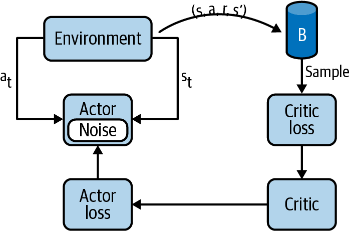
Figure 6-2. A simplified depiction of the DDPG algorithm.

Algorithm 6-3 provides the full DDPG implementation.

Algorithm 6-3. DDPG algorithm

$$\begin{array}{cc}\hfill \text{1:}& 𝐢𝐧𝐩𝐮𝐭\text{:}\text{an}\text{actor}\text{neural}\text{network,}{\mu }_{{\theta }_{\mu }}\left(s\right)\text{,}\text{with}\text{weights}{\theta }_{\mu }\text{,}\hfill \\ & \text{a}\text{critic}\text{neural}\text{network,}{Q}_{{\theta }_Q}(s,a)\text{,}\text{with}\text{weights}{\theta }_Q\text{,}\hfill \\ & \text{a}\text{replay}\text{buffer,}B\text{,}\hfill \\ & \text{the}\text{size}\text{of}\text{a}\text{training}\text{minibatch,}N\text{,}\hfill \\ & \text{the}\text{network}\text{update}\text{rate,}\tau \text{,}\hfill \\ & \text{the}\text{discount-rate}\text{parameter,}\gamma \text{,}\hfill \\ & \text{and}\text{a}\text{noise}\text{function}\text{for}\text{exploration,}𝒩\hfill \\ \hfill \text{2:}& \text{Initialize}{\theta }_{\mu }\text{,}{\theta }_Q\text{,}R\text{,}\hfill \\ & \text{and}\text{the}\text{target}\text{weights,}{\theta }_{\mu }^{\text{'}}\leftarrow {\theta }_{\mu }\text{,}{\theta }_Q^{\text{'}}\leftarrow {\theta }_Q\hfill \\ \hfill \text{3:}& 𝐥𝐨𝐨𝐩\text{:}\text{for}\text{each}\text{episode}\hfill \\ \hfill \text{4:}& \text{Initialize}s\hfill \\ \hfill \text{5:}& 𝐰𝐡𝐢𝐥𝐞s\text{is}\text{not}\text{terminal:}\hfill \\ \hfill \text{6:}& a\leftarrow {\mu }_{{\theta }_{\mu }}\left(s\right)+𝒩\hfill \\ \hfill \text{7:}& \text{Take}\text{action,}a\text{,}\text{and}\text{observe}r,s\text{'}\hfill \\ \hfill \text{8:}& \text{Store}(s,a,r,s^{\text{'}})\text{in}B\hfill \\ \hfill \text{9:}& \text{Sample}\text{a}\text{random}\text{minibatch}\text{of}N\text{transitions,}(s_i,a_i,r_i,s_i^{\text{'}})\text{,}\text{from}B\hfill \\ \hfill \text{10:}& y_i\leftarrow r_i+\gamma Q_{{\theta }_Q^{\text{'}}}\left(s_i^{\text{'}},{\mu }_{{\theta }_{\mu }^{\text{'}}}\left(s_i^{\text{'}}\right)\right)\text{(Note}\text{the}\text{target}\text{weights}\text{and}\text{buffer}\text{data)}\hfill \\ \hfill \text{11:}& \text{Update}\text{the}\text{critic}\text{by}\text{minimizing:}\frac{1}{N}\sum _i{\left(y_i-Q_{{\theta }_Q}(s_i,a_i)\right)}^2\hfill \\ \hfill \text{12:}& \text{Update}\text{the}\text{actor}\text{by}\text{minimizing:}\frac{1}{N}\sum _i{\left({\nabla }_{{\theta }_{\mu }}{Q}_{{\theta }_Q}\left(s_i,{\mu }_{{\theta }_{\mu }}\left(s_i\right)\right)\right)}^2\hfill \\ \hfill \text{13:}& {\theta }_Q^{\text{'}}\leftarrow \tau {\theta }_Q+(1-\tau ){\theta }_Q^{\text{'}}\hfill \\ \hfill \text{14:}& {\theta }_{\mu }^{\text{'}}\leftarrow \tau {\theta }_{\mu }+(1-\tau ){\theta }_{\mu }^{\text{'}}\hfill \\ \hfill \text{15:}& s\leftarrow s\text{'}\hfill \end{array}$$

To use Algorithm 6-3 in your applications you first need to define a neural architecture that matches your problem. You’ll need two networks, one for the actor (the policy) and one for the critic (an action-value function approximation). For example, if you were working with raw pixels, then you might use a convolutional neural network in the critic. If you’re working with customer information, then you might use a multilayer feed-forward network. For the policy, remember that DDPG is deterministic, so you want to predict a single action for a given state. Therefore, the number of outputs depends on your action space. The hyperparameters of the network are also very important. There should be enough capacity to approximate the complexities of your domain but you don’t want to overfit. The learning rate directly impacts the stability of the learning process. If you attempt to learn too quickly, you might find that it does not converge. The remaining inputs in step (1) of Algorithm 6-3 consist of the hyperparameters that control the learning and a noise function that enables exploration.

Steps (2) and (3) initialize the network weights and the replay buffer. The replay buffer must store new tuples and potentially pop off historical tuples when the buffer is full. It also needs to be able to randomly sample from that buffer to train the networks. You can initialize the network weights in different ways and they impact both stability and learning speed.¹⁰ Step (3) initializes copies of both the critic and actor networks, or target networks in the literature, to improve stability. In the rest of the algorithm, the copies are denoted by a ${}^{\text{'}}$ character. This is to save space, but they are easy to miss. If you create your own DDPG implementation, double-check that you are using the right network. Implementations often call the original networks local.

Step (6) uses the deterministic policy to predict an action. This is where the original algorithm introduces noise into that decision. But you may want to consider adding noise in different ways (see “Noisy Nets”, for example).

Step (8) stores the current tuple in the replay buffer and step (9) samples a batch of them ready for training. Many implementations delay the first training of the networks to allow for a more representative sample.

Step (10) marks the beginning of network training process. First it predicts the action value of the next state using the target networks and the current reward. Then step (11) trains the critic to predict that value using the local weights. If you combine steps (10) and (11) together you can see that this is the temporal-difference error.

Step (12) trains the actor network using the local weights by minimizing the gradient of the action-value function when using the actor’s policy. This is the equation from Equation 6-4 before applying the chain rule to move the policy gradient out of the action-value function. Implementations use this version because you can get the gradient of the action-value estimate from your DL framework by calling the gradient function. Otherwise you would have to calculate the gradient of the action-value function and the gradient of the policy.

Finally, steps (13) and (14) copy the target weights to the local weights. They do this by exponentially weighting the update; you don’t want to update the weights too quickly or the agent will never converge.

Twin Delayed DDPG

Twin delayed deep deterministic policy gradients (TD3) are, as the name suggests, an incremental improvement of DDPG. Like the Rainbow algorithm, Fujimoto et al. prove that three new implementation details significantly improve the performance and robustness of DDPG.11

Delayed policy updates (DPU)

The first and most interesting proposal is that actor-critic architectures suffer from the implicit feedback loop. For example, value estimates will be poor if the policy generating trajectories is suboptimal. But policies cannot improve if the value estimates are not accurate. In this classic “Which came first, the chicken or the egg?” scenario, Fujimoto et al. suggest that you wait for stable approximations before you retrain the networks. Statistical theory states that you need a representative sample before you can estimate a quantity robustly. The same is true here; by delaying updates, you improve performance (also see “Delayed Q-Learning”).

If you retrain your networks less frequently, performance increases. Training less, not more, is better in the long run. Initially this sounds counterintuitive, but I do have an analogy. When I work on complex projects, there are times when something fundamentally affects the work, like funding, for example. In these situations I have learned that knee-jerk reactions are unlikely to be optimal. They are emotionally driven and based upon uncertain, noisy information. Instead, I just listen and gather information. I defer any decisions until a later time. I find that by waiting a few days for the dust to settle, I have a much clearer picture of the situation. Delayed information has a lower variance, so my action predictions become more certain.

This also happens in actor-critic architectures. The implicit feedback loop increases the variance of the updates. When a network changes, the resulting change in actions and trajectories is uncertain. You need to wait a while to see what the effect is. One simple solution is to delay the updates. Retrain your deep learning neural networks after a specified amount of time.

Clipped double Q-learning (CDQ)

The second improvement implements double Q-learning (see “Double Q-Learning”). If you were to plot the action-value estimate against the true value, you would see that greedy methods tend to overestimate. Double Q-learning solved this by having two action-value estimates. When you retrain those estimates you use the other’s weights. But in deep architectures this doesn’t work so well, because the estimates are not independent. They use the same replay buffer and are both coupled to the generation policy. One simple solution is to pick the lowest action-value estimate. This prevents overestimation by actively underestimating. Despite the heavy-handed approach, the researchers found that it worked well in practice.

CDQ significantly improves performance in the Ant environment, which suggests that the action-value estimates are likely to be grossly overestimated. I propose that the reason for this is because the reward, which is typically the velocity of the ant, is not solely dependent on that single action. The ant has four legs, so if one of them produces a bad action, the other three can compensate and potentially lead to a good reward. This will mistakenly assign a positive reward to that bad action. CDQ mitigates this issue, by reporting the lowest possible value for any state-action pair, but you could also improve performance with a reward designed to isolate each leg (or joint). I suspect that further performance increases are possible in the Ant environment, or any environment with coupled actions, if you can make the action-reward assignment more independent.

Target policy smoothing (TPS)

The final and least significant improvement is to add noise to the action when predicting the action-value estimate. Because the policy is deterministic, it is very easy to repeatedly sample the same state and action. This leads to peaks in the action-value surface. The researchers suggested one way to smooth out the peak by adding noise to the action before predicting the value. Others have suggested directly smoothing the action-value estimate and adding noise to the network weights directly.

The evidence shows that adding TPS by itself does not improve results significantly. However, removing it from the TD3 algorithm does make a significant difference. I speculate that the reason for this is that it improves exploration. If there are peaks in the action-value estimate, then it would take a lot of visits to neighboring state-action pairs to smooth out that peak, which is unlikely given the large action space. Smoothing makes it easier for the policy to change its mind.

TD3 implementation

The implementation of TD3 is shown in Algorithm 6-4. This is similar to the implementation of DDPG except there is extra logic to handle the double Q-learning and delayed policy updates. The notation is consistent with the rest of the book, which means the algorithm looks slightly different compared to the original paper. You can see that the terminology is beginning to get complicated because of the various copies of data and parameters floating around. This makes it very easy to make an implementation mistake, so be careful.

Algorithm 6-4. TD3 algorithm

$$\begin{array}{cc}\hfill \text{1:}& 𝐢𝐧𝐩𝐮𝐭\text{:}\text{an}\text{actor}\text{neural}\text{network,}{\mu }_{{\theta }_{\mu }}\left(s\right)\text{,}\text{with}\text{weights}{\theta }_{\mu }\text{,}\hfill \\ & \text{two}\text{critic}\text{neural}\text{networks,}{Q}_{{\theta }_1}(s,a),Q_{{\theta }_2}(s,a)\text{,}\text{with}\text{weights}{\theta }_1,{\theta }_2\text{,}\hfill \\ & \text{a}\text{replay}\text{buffer,}B\text{,}\hfill \\ & \text{the}\text{size}\text{of}\text{a}\text{training}\text{minibatch,}N\text{,}\hfill \\ & \text{the}\text{network}\text{update}\text{rate,}\tau \text{,}\hfill \\ & \text{the}\text{discount-rate}\text{parameter,}\gamma \text{,}\hfill \\ & \text{a}\text{noise}\text{clipping}\text{threshold,}c\text{,}\hfill \\ & \text{and}\text{a}\text{noise}\text{function}\text{for}\text{exploration,}𝒩\hfill \\ \hfill \text{2:}& \text{Initialize}{\theta }_{\mu },{\theta }_1,{\theta }_2\text{,}\hfill \\ & \text{and}\text{the}\text{target}\text{weights,}{\theta }_{\mu }^{\text{'}}\leftarrow {\theta }_{\mu }\text{,}{\theta }_1^{\text{'}}\leftarrow {\theta }_1,{\theta }_2^{\text{'}}\leftarrow {\theta }_2\hfill \\ \hfill \text{3:}& 𝐥𝐨𝐨𝐩\text{:}\text{for}\text{each}\text{episode}\hfill \\ \hfill \text{4:}& \text{Initialize}s\hfill \\ \hfill \text{5:}& 𝐰𝐡𝐢𝐥𝐞s\text{is}\text{not}\text{terminal:}\hfill \\ \hfill \text{6:}& a\leftarrow {\mu }_{{\theta }_{\mu }}\left(s\right)+𝒩\hfill \\ \hfill \text{7:}& \text{Take}\text{action,}a\text{,}\text{and}\text{observe}r,s\text{'}\hfill \\ \hfill \text{8:}& \text{Store}(s,a,r,s^{\text{'}})\text{in}B\hfill \\ \hfill \text{9:}& \text{Sample}\text{a}\text{random}\text{minibatch}\text{of}N\text{transitions,}(s_i,a_i,r_i,s_i^{\text{'}})\text{,}\text{from}B\hfill \\ \hfill \text{10:}& {\tilde{a}}_i\leftarrow {\mu }_{{\theta }_{\mu }^{\text{'}}}\left(s_i^{\text{'}}\right)+clip(𝒩,-c,c)\text{(Target}\text{policy}\text{smoothing)}\hfill \\ \hfill \text{11:}& y_i\leftarrow r_i+\gamma \underset{j=1,2}{min}{Q}_{{\theta }_j^{\text{'}}}(s_i^{\text{'}},{\tilde{a}}_i)\text{(Clipped}\text{double}\text{Q-learning)}\hfill \\ \hfill \text{12:}& \text{Update}\text{both}\text{critics,}{\theta }_{j\leftarrow 1,2}\text{,}\text{by}\text{minimizing:}\frac{1}{N}\sum _i{\left(y_i-Q_{{\theta }_j}(s_i,a_i)\right)}^2\hfill \\ \hfill \text{13:}& iftmoddthen\text{:}\text{(Delayed}\text{policy}\text{update)}\hfill \\ \hfill \text{14:}& \text{Update}\text{the}\text{actor}\text{by}\text{minimizing:}\frac{1}{N}\sum _i{\left({\nabla }_{{\theta }_{\mu }}{Q}_{{\theta }_1}\left(s_i,{\mu }_{{\theta }_{\mu }}\left(s_i\right)\right)\right)}^2\hfill \\ \hfill \text{15:}& \text{Update}\text{both}\text{critics,}{\theta }_{j\leftarrow 1,2}\text{:}{\theta }_j^{\text{'}}\leftarrow \tau {\theta }_j+(1-\tau ){\theta }_j^{\text{'}}\hfill \\ \hfill \text{16:}& {\theta }_{\mu }^{\text{'}}\leftarrow \tau {\theta }_{\mu }+(1-\tau ){\theta }_{\mu }^{\text{'}}\hfill \\ \hfill \text{17:}& endif\hfill \\ \hfill \text{18:}& s\leftarrow s\text{'}\hfill \end{array}$$

In step (1) you now have to pass in two critic networks, denoted by the parameters ${\theta }_1$ and ${\theta }_2$. Most implementations expect you to pass in two independent DL networks and typically these have exactly the same architecture. But don’t let this stop you from trying different architectures or possibly a multihead architecture.

The original algorithm clips the action noise to keep the result close to the original action. The intent is to prevent the agent from choosing invalid actions. Most implementations set this value to match the environment’s action space. I tentatively suggest that because you control the design of your noise function, clipping is unnecessary. Choose a noise function that matches your action space and smoothing goals, then reuse the standard deterministic action function from DDPG [step (6)].

In step (11) note that the predicted value is the minimum value from both critics from the target networks. In other words, pick the lowest action-value estimate; this is more likely to be correct due to the overestimation bias. Step (12) updates both critics using this prediction of the discounted reward. This helps to restrain the network that is doing the overestimation.

The inner loop after step (13) occurs one every $d$ iterations; this delays the policy update. Line (14) is interesting because it uses the first critic to update the policy, not the critic with the minimum value. I suspect the reasoning here is that because the overestimating network is constrained by step (12), it doesn’t make any difference if you pick network one or two, in the long run. Either network is as likely to overestimate. But you might find minor performance gains here by choosing which network to use more intelligently.

All other lines are the same as DDPG.

Tip

Always refer to the original paper and add enough monitoring code to verify your implementation. I find that unfolding loops and calculating by hand is the best way to verify that code is working as I expect.

Case Study: Recommendations Using Reviews

In the era of information overload, users are increasingly reliant on recommendation algorithms to suggest relevant content or products. More recently, services like YouTube and TikTok have begun to leverage interactive recommender systems, which continuously recommend content to individual users based upon their feedback. State-of-the-art non-RL methods attempt to build models that map users to items, leverage locally correlated patterns using convolutional filters, or use attention-based sequential prediction models. Out of these, the sequential models perform the best because they adapt to recurrent feedback. But these methods train offline and must be retrained often to provide up-to-date recommendations. Combined with the complexity of the deep learning models, this adds up to a large training cost.

RL is a natural fit for this type of problem because feedback can be accommodated directly through the reward definition. Wang et al. propose one example in which they make things more interesting by proposing to use text as a feedback mechanism, rather than the usual up- or downvote. They suggest that in the real world sparse voting can severely degrade performance. Instead, they suggest that textual information like reviews and item descriptions contains more information and is less sensitive to sparsity.12

Wang et al. formulate the problem using a Markov decision process where the state is the interaction between a user and the recommender system, the action is a number of recommended items, and the reward is determined by the user feedback.

The primary issue, as noted by other recommendation papers, is the high-dimensionality introduced by the sheer numbers of users and items. Wang et al. take the route of using a word embedding to map the item text and user review into a feature vector, then use a clustering method to reduce the feature vector into a manageable number of groups.

Wang et al. then choose DDPG as their algorithm of choice to be able to learn policies in a high-dimensional, continuous action space. They needed the ability to predict continuous actions to work with the continuous user-embedding space. They then combine the set of items with the action to produce an ordered list of items ready to present to the user. Over time the policy learns what actions (i.e., user-item embedding) are preferred given the user and candidate items as a state. As new user feedback or items are added, the policy is able to change to meet the new demands of the users or propose new recommended items.

Unfortunately, Wang et al. only tested this in a simulation. They used a dataset of Amazon products that had reviews. They used the review score to denote a positive or negative review and reward based upon whether the user’s well-reviewed item was in the top results. Their method produced results that beat all other state-of-the-art ML implementations.

I like the idea of incorporating textual information as a way to reduce the sparsity of the problem. But I wish that they had tested this in a real environment. Of course, not everyone has access to YouTube or Amazon to be able to test these things out. Only then would we be able to see how well this really performs. My guess is that it should perform at least as well as any highly tuned ML recommender, and probably beat it, with the added benefit of not requiring retraining. And remember that this is without any special tuning or fancy neural networks. The policy was a vanilla multilayer perceptron. I’m also confident that there are improvements to be made, too. Other researchers have looked at tackling the dimensionality problem head on and don’t have to perform clustering to create recommendations.¹³

You may also be interested in RecSim, a configurable simulation platform for recommender systems.¹⁴

Improvements to DPG

You can apply many of the fundamental improvements seen in previous chapters like different exploration strategies, or different ways to represent the expected reward. These can all affect and improve performance. For example, distributed distributional deterministic policy gradients from Barth-Maron et al. not only introduce parallelism (see “Scaling RL”) but add distributional RL (see “Distributional RL”) and $n$-step updates (see “n-Step Algorithms”).¹⁵ Deterministic value-policy gradients by Cai et al. prove that you can use deterministic algorithms for infinite-horizon environments and add $n$-step updates like a cherry on top of a cake.¹⁶

But there is one fundamental problem that hasn’t been fixed, at least not in this context. Despite all their benefits, off-policy algorithms are the same as delta-wing jets like the Eurofighter Typhoon: they are inherently unstable. Without artificial control they will diverge and crash. The Eurofighter achieves this with a complex flight control system. Off-policy algorithms achieve this by slowing down the rate at which parameters update in the neural networks to the point where updates are actively skipped. Surely this is slowing down learning. Is there a better way?

Trust Region Methods

PG algorithms learn to make better choices by following the gradient of a policy toward higher predicted values, weighted by some measure of expected return. The following methods all use the advantage function, $A(s,a)$, but you could plausibly choose any PG interpretation (see “A Comparison of Basic Policy Gradient Algorithms”).

Delegating Gradient Calculations to a Library

Q-learning and vanilla policy gradient algorithms can solve a significant percentage of problems. But the main reason for developing more advanced RL algorithms is so that agents can tackle more complex tasks, like generating policies for a pick-and-place robot.

A problem that necessitates a more complex RL algorithm also implies that you need more complex approximators. These become harder to encode, manage, and calculate gradients for (in the case of policy gradients) and at some point, which is exceedingly fuzzy, this becomes too difficult. It is increasingly tempting to entrust all of this to a deep learning framework. Yes, neural networks have their problems, but these frameworks make it incredibly easy to create, manage, and update highly complex approximators.

Therefore, in complex policy gradient algorithms, RL practitioners tend to ignore the gradient operator (the $\nabla$) and instead present a loss function (the mathematics inside the $\nabla$). The gradient calculation is outsourced to the reverse-mode auto-differential algorithm provided by TensorFlow, PyTorch, and the like.

Equation 6-5 presents the A2C update in the form of a loss function, where $A_{\pi }(s,a)\doteq Q_{\pi }(s,a)-V_{\pi }\left(s\right)$. The advantage function has an intuitive interpretation. Actions with a value estimate greater than zero are better than average. They will result in good performance, on average. Actions lower than zero will, on average, result in poor performance.

Equation 6-5. Advantage actor-critic policy gradient

$$L^{PG}\left(\theta \right)\doteq {𝔼}_{{\pi }_{\theta }}\left[ln{\pi }_{\theta }(a\mid s)A_w(s,a)\right]$$

Using the advantage function in combination with the policy gradient forces the policy toward producing more performant actions and away from poorly performing actions. Compare this against using the action-value function instead. For many problems it is likely that all actions have a positive value; if you wander randomly you will eventually stumble across a reward. So if you used that here, like in a vanilla actor-critic, then it will move the policy toward all of these eventualities, but at different rates. This can cause value estimates to increase infinitely and can be unstable when near-optimal, which is why you need to use discounting. The advantage function provides a natural damping. If the policy ever goes too far, like if it makes a massive mistake, the advantage function will kick it back on track. A bad move in policy will manifest in poor results that yield a negative advantage and therefore a negative gradient, which pushes the policy back to better performance.

But you have to be careful not to update the policy too quickly. The advantage function is an approximation (a supervised model), so you must take the result with a pinch of salt. It is noisy and you don’t want to ruin your policy with a single bad step. Which leads to a question: how do we quantify the size of a step?

The vanilla advantage actor-critic is promoting the trajectories that yield positive advantages; it is trying to maximize future returns. It achieves this by using an optimization function that moves up the gradient of the policy, which itself depends on the advantages. This gradient is a local linear estimate of a complex nonlinear function. You can’t jump directly from where you were to where you want to go, because it is likely that you will end up in the middle of nowhere.

It’s like if you go hiking and you set your direction by taking a single compass reading at the start. You will end up miles away from your destination because you can’t pick a bearing with enough precision. To solve this problem you take new readings every kilometer or so. You introduce a step size and iteratively take measurements. In this analogy, the step size is a Euclidian distance, the hypotenuse of a triangle, measured in meters. Stochastic gradient ascent/descent uses the same Euclidian distance, but the units are much more complex to interpret. The cost function is in units of policy parameters, which themselves have a complex interaction with states to produce action probabilities.

A related problem is that the data you are using to train your models is nonstationary. For example, consider the common situation where you have sparse rewards (your policy does not observe a reward for a long time). You probably don’t want to alter the policy much while it is exploring, so the step size should be small. But when you do find a reward, you want to update the policy significantly, to take advantage of that new knowledge. But by how by much? If you make a mistake and update it too much, then the policy might become so bad that it becomes impossible to find a good reward again.

These problems make it hard to choose a single step size that works in all situations. Practitioners usually treat this as a hyperparameter and scan over a range of values. In other words, brute force.

Trust region methods attempt to solve this problem by attempting to specify a region in parameter space which gradient steps can be trusted. You can use this information to dynamically alter the step size so that the parameters change quickly when gradients are trusted and slowly when they are not. Then you can find ways to quantify that trust, the first of which is based upon using the Kullback–Leibler divergence to measure the difference between two policies.

Kullback–Leibler Divergence

The Kullback–Leibler (KL) divergence is often described as a measure of “surprise” when comparing two distributions. When the distributions are the same, then the KL divergence is zero. When the distributions are dramatically different, the KL divergence is large.

It can also be used to calculate the extra number of bits required to describe a new distribution given another. If the distributions are the same, then you require no extra bits to differentiate the new distribution. If the distributions are different, then you would need many new bits.

For example, if you had a special coin that only ever landed on heads, then you would need zero bits to represent the coin’s states. There is only one state—it is always going to be heads—so you need zero bits, just the value zero, to encode that state. If you compared that to a fair coin, you would now have two states, so you would need one full bit to represent those states. In this hypothetical example, the KL divergence between these two distributions is 1 (hypothetical because as one state approaches zero, the division in the KL divergence algorithm will produce a nan).

Equation 6-6 presents the divergence calculation. $\parallel$ represents the divergence operator, which tells you to calculate the divergence between this and that. You can use any base for the logarithm, but most people use a base of 2 (log2), which represents the number of bits.

Equation 6-6. Kullback–Leibler divergence

$$D_{KL}(P\parallel Q)\doteq \sum _{x\in 𝒳}P\left(x\right)log\left(\frac{P\left(x\right)}{Q\left(x\right)}\right)$$

KL divergence experiments

Consider the following two experiments where I flip coins and roll dice. KL divergence is a measure of how different distributions are, so flipping two fair dice should result in a divergence of zero. Then I simulate a biased coin that is weighted toward landing on tails.

In the second experiment I simulate three six-sided dice. The first is a standard, fair die. The second is a fair die but produces double the value of a standard six-sided die. In other words, the probabilities are similar but the distributions do not align. The third die produces standard values but is biased to produce more sixes than you would expect.

Figure 6-3 shows histograms of these experiments where the KL divergence is shown in brackets. As you would expect, the KL divergence between two fair coins is near zero. However, when comparing with the biased coin, the divergence is nonzero.

Comparing fair and biased dice produces the same nonzero result. But note the result from the comparison between the fair die and the die that produces values that lie outside the range of the fair die. The KL divergence is near zero. This is because where it does overlap, it has the same uniform distribution. This is because KL divergence does not measure the spread between distributions; if you’re interested in that, use the total variance divergence instead.

Figure 6-3. Calculating the KL divergence for simulations of coins and dice.

Natural Policy Gradients and Trust Region Policy Optimization

Natural policy gradients (NPG) introduced the idea that you can quantify step size not in terms of policy parameter space, but in terms of a metric based upon the distance between the current policy and the policy after updating by a gradient step.17

Figure 6-4 shows an example of the difference between standard policy gradients and natural policy gradients. The contours represent the value of a particular state and the arrows show the direction of the gradient as defined by the type of gradient calculation. It demonstrates that the gradients change direction when you compute the differential with respect to a different feature.

You can estimate the distance between two policies by comparing the distributions of the generated trajectories using one of many statistical measures to compare two distributions. But the trust region policy optimization (TRPO) algorithm uses KL divergence.¹⁸ Recall that optimization algorithms measure step sizes by the Euclidian distance in parameter space; steps have units of $\delta \theta$. TRPO suggests that you can constrain, or limit this step size according to the change in policy. You can tell the optimization algorithm that you don’t want the probability distribution to change by a large amount. Remember, this is possible because policies are action-probability distributions.

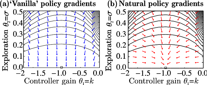
Figure 6-4. An example of the standard (left) and natural (right) policy gradients produced in a simple two-dimensional problem. Image from Peters et al. (2005) with permission.¹⁹

Equation 6-7 presents a slight reformulation of the A2C policy gradient. If you look at the derivation of the policy gradient theorem in Equation 5-3, at the end I introduced a logarithm to simplify the mathematics. Technically, this gradient is computed using trajectories sampled from an old policy. So if you undo the last step (chain rule), you end up with the same equation, but the use of the old policy parameters is more explicit.

Equation 6-7. Reformulated advantage actor-critic loss function

$$\begin{array}{cc}\hfill \nabla J\left(\theta \right)& ={𝔼}_{{\pi }_{\theta }}\left[\nabla ln{\pi }_{\theta }(a\mid s)A_w(s,a)\right]\hfill \\ & ={𝔼}_{{\pi }_{\theta }}\left[\frac{\nabla {\pi }_{\theta }(a\mid s)}{{\pi }_{{\theta }_{\text{old}}}(a\mid s)}{A}_w(s,a)\right]\hfill \end{array}$$

Next, because you can delegate the gradient calculation, you can rewrite Equation 6-7 in terms of the objective, which is to maximize the expected advantages by altering the policy parameters, $\theta$. You can see the result in Equation 6-8.

Equation 6-8. Presenting A2C in terms of maximization of the objective

$$\begin{array}{cc}\hfill \underset{\theta }{maximize}{L}^{PG}\left(\theta \right)& ={𝔼}_{{\pi }_{\theta }}\left[\frac{{\pi }_{\theta }(a\mid s)}{{\pi }_{{\theta }_{\text{old}}}(a\mid s)}{A}_w(s,a)\right]\hfill \end{array}$$

An alternative interpretation of Equation 6-8 is that this is importance sampling of the advantages (not the gradient, like in “Off-Policy Actor-Critics”). The expected advantage is equal to the advantage of the trajectories sampled by the old policy, adjusted by importance sampling, to yield the results that would be obtained if you used the new policy.

Equation 6-9 shows the loss function for the NPG algorithm, which as you can see is the same as Equation 6-8, but with a constraint (a mathematical tool that limits the value of the equation above it). NPG uses a constraint based upon the KL divergence of the new and old policies. This constraint prevents the divergence from being greater than $\delta$.

Equation 6-9. Natural policy gradients optimization loss function

$$\begin{array}{cc}\hfill \underset{\theta }{maximize}{L}^{TRPO}\left(\theta \right)={𝔼}_{{\pi }_{\theta }}& \left[\frac{{\pi }_{\theta }(a\mid s)}{{\pi }_{{\theta }_{\text{old}}}(a\mid s)}{A}_w(s,a)\right]\hfill \\ \hfill subjectto{𝔼}_{{\pi }_{\theta }}& \left[\text{KL}\left[{\pi }_{{\theta }_{\text{old}}}(·\mid s)\parallel {\pi }_{\theta }(·\mid s)\right]\right]\le \delta \hfill \end{array}$$

This is all well and good, but the major problem is that you can’t use stochastic gradient descent to optimize constrained nonlinear loss functions. Instead, you have to use conjugate gradient descent, which is similar to standard gradient descent but you can include a constraint.

TRPO adds a few bells and whistles like an extra linear projection to double-check that the step really does improve the objective.

The major problem, however, is that the implementation involves a complex calculation to find the conjugate gradients, which makes the algorithm hard to understand and computationally complex. There are other issues too, like the fact that you can’t use a neural network with a multihead structure, like when you predict action probabilities and a state-value estimate, because the KL divergence doesn’t tell you anything about how you should update the state-value prediction. In practice, then, it doesn’t work well for problems where good estimates of a complex state-value space are important, like the Atari games.

These issues prevent TRPO from being popular. You can read more about the derivation of NPG and TRPO in the resources suggested in “Further Reading”. Thankfully, there is a much simpler alternative.

Proximal Policy Optimization

One of the main problems with NPG and TRPO is the use of conjugate gradient descent. Recall that the goal is to prevent large changes in the policy, or in other words, to prevent large changes in the action probability distribution. NPG and TRPO use a constraint on the optimization to achieve this, but another way is to penalize large steps.

Equation 6-8 is a maximization; it’s trying to promote the largest advantage estimates, so you could add a negative term inside the loss function that arbitrarily decreases the advantage value whenever policies change too much. Equation 6-10 shows this in action, where the constraint is moved to a negation and an extra term, $\beta$, controls the proportion of penalization applied to the advantages.

The major benefit is that you can use standard gradient ascent optimization algorithms again, which dramatically simplifies the implementation. However, you would struggle to pick a value for $\beta$ that performs consistently well. How big of a penalization should you apply? And should that change depending on what the agent is doing? These are the same problems presented at the start of this section, which makes this implementation no better than picking a step size for A2C.

Equation 6-10. Penalizing large changes in policy

$$\begin{array}{cc}\hfill \underset{\theta }{maximize}{𝔼}_{{\pi }_{\theta }}& \left[\frac{{\pi }_{\theta }(a\mid s)}{{\pi }_{{\theta }_{\text{old}}}(a\mid s)}{A}_w(s,a)-\beta \text{KL}\left[{\pi }_{{\theta }_{\text{old}}}(·\mid s)\parallel {\pi }_{\theta }(·\mid s)\right]\right]\hfill \end{array}$$

But do not despair; Equation 6-10 highlights an important idea. It shows that you can add arbitrary functions to influence the size and direction of the step in an optimization algorithm. This opens a Pandora’s box of possibilities, where you could imagine adding things like (simpler) functions to prevent large steps sizes, functions to increase step sizes when you want more exploration, and even changes in direction to attempt to explore different regions in policy space. Proximal policy optimization (PPO) is one such implementation that adds a simpler penalization, an integrated function to allow for multihead networks, and an entropy-based addition to improve exploration.²⁰

PPO’s clipped objective

Schulman et al. proposed that although TRPO was technically more correct, it wasn’t necessary to be so fancy. You can use the importance sampling ratio as an estimate of the size of the change in the policy. Values not close to 1 are indicative that the agent wants to make a big change to the policy. A simple solution is to clip this value, which constrains the policy to change by a small amount. This results in the a new clipped loss function shown in Equation 6-11.

Equation 6-11. Clipping large changes in policy according to the importance sampling ratio

$$L^{CLIP}\left(\theta \right)\doteq 𝔼\left[min(r\left(\theta \right)A(s,a),clip(r\left(\theta \right),1-ϵ,1+ϵ)\widehat{a}(s,a))\right]$$

$r\left(\theta \right)\doteq {\pi }_{\theta }(a\mid s)/{\pi }_{{\theta }_{\text{old}}}(a\mid s)$ is the importance sampling ratio. Inside the expectation operator there is a min function. The righthand side of min contains an importance sampling ratio that is clipped whenever the value veers more than $ϵ$ away from 1. The lefthand side of the min function is the normal unclipped objective. The reason for using min is so that the objective results in providing the worst possible loss for these parameters, which is called a lower bound or pessimistic bound.

At first this sounds counterintuitive. In situations like this I find it useful to imagine what happens when you test the function with different inputs. Remember that the advantage function can have positive and negative values. Figure 6-5 shows the clipped loss when the advantages are positive (left) and negative (right).

Figure 6-5. A plot of the clipped PPO loss when advantages are positive (left) or negative (right).

A positive advantage (left) indicates that the policy has a better than expected effect on the outcome. Positive loss values will nudge the policy parameters toward these actions. As the importance sampling ratio [$r\left(\theta \right)$] increases, the righthand side of the min function will clip at the $1+ϵ$ point and produce the lowest loss. This has the effect of limiting maximum loss value and therefore the maximum change in parameters. You don’t want to change parameters too quickly when improving, because a jump too big might push you back into poor performance. Most of the time the ratio will be near 1. The $ϵ$ allows a little room to improve.

A negative advantage suggests that the policy has a worse than expected effect on the outcome. Negative loss values will push the policy parameters away from these actions. At high ratios, the lefthand side of the min function will dominate. Large negative advantages will push the agent back toward more promising actions. At low ratios, the righthand side of the min function dominates again and is clipped at $1-ϵ$. In other words, if the distribution has a low ratio (meaning there is a significant difference in the old and new policies), then the policy parameters will continue to change at the same rate.

But why? Why do this at all? Why not just use the raw advantage? Schulman et al. set out to establish and improve a lower bound on performance, a worst-case scenario. If you can design a loss function that guarantees improvement (they did) then you don’t need to care so much about the step size.

Figure 6-6 is a depiction of this problem using notation from TRPO. $\theta$ are the parameters of the current policy. Ideally, you want to observe the curve labeled $\eta \left(\theta \right)$, which is the true performance using the parameters $\theta$. But you can’t because it would take too long to estimate that complex nonlinear curve at every step. A faster method is to calculate the gradient at this point, which is shown as the line labeled $L\left(\theta \right)$. This is the gradient of the A2C loss. If you take a large step on this gradient, then you could end up with parameters that over- or undershoot the maximum. The curve labeled $L\left(\theta \right)-\beta KL$ is the TRPO lower bound. It is the A2C gradient with the KL divergence subtracted. You can see that no matter what step size you chose, you would still end up somewhere within $\eta \left(\theta \right)$; even if the agent makes a really bad step, it is constrained to end up somewhere within that lower bound, which isn’t too bad.

Figure 6-6. A depiction of the TRPO lower bound with gradients.

PPO achieves a similar lower bound by ignoring the importance sampling when the policy is improving (take bigger steps), but includes it and therefore accentuates the loss when the policy is getting worse (provide a lower bound). I like to think of it as a buildup of pressure; PPO is pressuring the advantages to improve.

PPO’s value function and exploration objectives

Most techniques for computing the advantages use an approximation to estimate the state-value function. At this point you’ve probably resigned to using a neural network, so it makes sense to use the same network to predict policy actions and the state-value function. In this scenario PPO includes a squared-loss term in the final objective to allow the DL frameworks to learn the state-value function at the same time as learning the policy: $L^{VF}\left(\theta \right)\doteq {(V_{\theta }\left(s\right)-V^{target})}^2$.

PPO also includes a term in the final objective that calculates the entropy of a policy, $\mathscr{H}\left[{\pi }_{\theta }\right]\left(s\right)$.²¹ This improves exploration by discouraging premature convergence to suboptimal deterministic policies. In other words, it actively discourages deterministic polices and forces the agent to explore. You will learn more about this idea in Chapter 7.

You can see the final PPO objective function in Equation 6-12. $C_1$ and $C_2$ are hyperparameters that control the proportion of the loss function attributed to the state-value loss and the entropy loss, respectively.

Equation 6-12. The final objective function for PPO

$$L^{CLIP+VF+S}\left(\theta \right)\doteq 𝔼\left[L^{CLIP}\left(\theta \right)+C_1{L}^{VF}\left(\theta \right)+C_2\mathscr{H}\left[{\pi }_{\theta }\right]\left(s\right)\right]$$

Algorithm 6-5 shows the deceptively simple pseudocode from the original paper by Schulman et al.²² It neglects implementation details like the policy and value function approximation, although it does assume a deep-learning–based implementation to provide the automatic differentiation. Note that the algorithm does have an implicit delayed update in there; it iterates for $T$ time steps before retraining the weights. But it does not concern itself with any other extensions (for example, determinism, replay buffers, separate training networks, distributions of actions/rewards, and so on). Any of these could improve performance for your particular problem.

What is interesting is the use of multiple agents in step (2). I haven’t talked much about asynchronous methods, but this is a simple way to improve the learning speed (in wall clock time). Multiple agents can observe different situations and feed that back into a central model. I discuss this idea in more depth in “A Note on Asynchronous Methods”.

Schulman et al. used values of between 0.1 and 0.3 for the divergence clipping hyperparameter, $ϵ$. The hyperparameter $C_1$ depends on whether you are using the same neural network to predict the policy and the state-value function. Schulman et al. didn’t even need to use an entropy bonus in some of their experiments and set $C_2\doteq 0$. There is no right answer, so use a hyperparameter search to find the optimal values for your problem.

Algorithm 6-5. Asynchronous PPO algorithm

$$\begin{array}{cc}\hfill \text{1:}& 𝐟𝐨𝐫\text{iteration}\doteq 0,1,\cdots \text{:}\hfill \\ \hfill \text{2:}& 𝐟𝐨𝐫\text{agent}\doteq 0,1,\cdots ,N-1\text{:}\hfill \\ \hfill \text{3:}& \text{Run}\text{policy}{\pi }_{{\theta }_{old}}\text{in}\text{environment}\text{for}T\text{time}\text{steps}\hfill \\ \hfill \text{4:}& \text{Compute}\text{advantage}\text{estimates}{A}_0,\cdots ,A_{T-1}\hfill \\ \hfill \text{5:}& \text{Optimize}L\text{with}\text{respect}\text{to}\theta \text{,}\text{for}K\text{epochs}\text{and}\text{minibatch}\text{size}M\le NT\hfill \\ \hfill \text{6:}& {\theta }_{old}\leftarrow \theta \hfill \end{array}$$

Example: Using Servos for a Real-Life Reacher

You have probably noticed that the majority of RL examples use simulations. This is mostly for practical purposes; it is much easier, cheaper, and faster to train in a simulated environment. But you can easily apply RL to problems that have a direct interface with real life. One of the most common examples of RL in industry is robotic control because RL is especially well suited to deriving efficient policies for complex tasks.

Academia has attempted to standardize robotics platforms to improve reproducibility. The ROBEL platform is one notable example of three simple, standardized robots that are capable of demonstrating a range of complex movements.²³ But even though they are “relatively inexpensive,” the $3,500 cost for D’Claw is a large price to justify.

These two challenges, the lack of real-life RL examples and the cost, were the basis for the next experiment. I wanted to re-create a typical RL experiment, but in real life, which lead me back to the classic CartPole and Reacher problems. Second, the high cost of D’Claw is primarily due to the expensive servo motors. For this experiment I only need a single servo motor and driver, which can be both purchased for less than $20. Full details of the hardware setup can be found on the accompanying website (see “Supplementary Materials”).

Experiment Setup

This experiment consists of a simulated and a real-life servo motor, which I drive toward a preset goal. Servo motors are like standard DC motors, except they have extra gearing and controls in place to provide accurate control. The servos I used also had positional feedback, which is not found in cheaper servos. Figure 6-7 shows a video of the servo motor while being trained.

Figure 6-7. A video of the PPO agent training the movement of a servo motor.

The state is represented by the current position of the servo and a fixed goal that is changed every episode. There is one action: the position of the servo. States and actions are normalized to fall within the range of –1 to 1. The reward is the negative Euclidian distance to the goal, a classic distance-to-goal metric that is used in many robotics examples. The episode ends when the servo moves within 5% of the goal position. Therefore the goal is to train an agent to derive a policy that moves to the precise position of the goal in the lowest number of moves.

This problem statement is not precisely the same as CartPole or Reacher. But the idea of training a robot to move to achieve a desired goal is a common requirement. The single servo makes the problem much easier to solve and you could handcode a policy. But the simplicity makes it easy to understand and more complicated variants are just an extension of the same idea.

RL Algorithm Implementation

Tip

Always try to solve the next simplest problem. RL is especially difficult to debug because there are so many feedback loops, hyperparameters, and environmental intricacies that fundamentally alter training efficiency. The best mitigation is to take baby steps and verify simpler problems are working before you move onto something more complex.

My first attempt at this problem involved trying to learn to move toward a goal that was completely fixed, for all episodes. I wanted to use PPO for this example. I chose a value of –1 because the random initializations would often accidentally lead to a policy that moved to 0 every step. This means that the agent has to learn an incredibly simple policy: always predict an action of –1. Easy right?

Incredibly, it didn’t converge. If I were less tenacious then I would hang up my engineering hat and retire. In general, I find that most problems involve an error between brain and keyboard. So I started debugging by plotting the predicted value function and the policy, the actual actions that were being predicted for a given observation, and I found that after a while the value function was predicting the correct values but the policy was just stuck. It wasn’t moving at all. It turned out that the default learning rate (stable-baselines, PPO2, 2.5e – 4) is far too small for such a simple problem. It wasn’t that the agent failed to learn, it was just learning too slowly.

After increasing the learning rate massively (0.05)to match the simplicity of the problem, it solved it in only a few updates.

The next problem was when I started tinkering with the number of steps per update and the minibatch size. The number of steps per update represents how many observations are sampled before you retrain the policy and value approximators. The minibatch size is the number of random samples passed to the training.

Remember that PPO, according to the paper implementation, does not have any kind of replay buffer. The number of steps per update represents the size of the minibatch used for training. If you set this too low, then the samples are going to be correlated and the policy will never converge.

You want to set the number of steps parameter to be greater than the minibatch size (so samples are less correlated) and ideally capture multiple episodes to again de-correlate. Another way to think about this is that each episode captured during an update is like having multiple independent workers. More independent workers allow the agent to average over independent observations and therefore break the correlation, with diminishing returns.

The minibatch size impacts the accuracy of the policy and value approximation gradients, so a larger value provides a more accurate gradient for that sample. In machine learning this is considered to be a good thing, but in RL it can cause all sorts of stability issues. The policy and value approximations are valid for that phase of exploration only. For example, on a complex problem with large state spaces, it is unlikely that the first sample is representative of the whole environment. If you use a large minibatch size it will reinforce the current policy behavior, not push the policy toward a better policy. Instead, it is better to use a lower minibatch size to prevent the policy from overfitting to a trajectory. The best minibatch size, however, is problem and algorithm dependent.24

For the problem at hand, I set the minibatch size very low, 2 or 4 in most experiments, so that I could retrain often and solve the problem quickly, and the number of steps to 32 or 64. The agent was easily able to solve the environment in this many steps so it was very likely that multiple episodes were present within a single update.

Finally, since the resulting policy was so easy to learn I dramatically reduced the size of the policy and value function networks. This constrained them both and prevented overfitting. The default implementation of a feed-forward multilayer perceptron in stable-baselines does not have any dropout, so I also forced the network to learn a latent representation of the data by using an autoencoder-like fan-in.

Figure 6-8 shows the final policy, which I generated by asking for the predicted action for all position observations for a fixed goal of –1. After only 20 steps of the motor, PPO has learned a policy that produces an action of –1 for all observations.

Figure 6-8. The final policy of the fixed goal experiment. The x-axis is the current observation of the position. The y-axis is the resulting action from the policy. There is a straight line at the –1 action, which correctly corresponds to the goal of –1.

Increasing the Complexity of the Algorithm

Now that I have verified that the hardware works and the agent is able to learn a viable policy, it is time to take the next step and tackle a slightly more difficult problem.

I now expand the problem by generating random goals upon every episode. This is more challenging because the agent will need to observe many different episodes and therefore multiple goals to learn that it needs to move to an expected position. The agent won’t know that there are different goals until it encounters different goals.

The agent also needs to generalize. The goals are selected uniformly to lie between –1 and 1. This is a continuous variable; the agent will never observe every single goal.

But the goal is still simple, however. The agent has to learn to move to the position suggested by the goal. It is a one-to-one mapping. But this poses a small challenge to RL agents because they don’t know that. The agents are equipped to map a very complex function. So similar to before I will need to constrain that exploration to the problem at hand.

From a technical perspective this is an interesting experiment because it highlights the interplay between the environment dynamics and the agent’s hyperparameters. Despite this being an easy function to learn (a direct mapping), the agent’s exploration and interaction adds a significant amount of noise into the process. You have to be careful to average out that noise. In particular, if the learning rate is too high, then the agent tends to continuously update its value and policy networks, which results in a policy that dances all over the place.

The number of steps is important,too. Previously, it was easy to complete an episode, since there was always a single goal. But now the goal could be anywhere, so an episode can take a lot more time early on in the training. This, coupled with a high learning rate, could lead to samples that are changing rapidly.

I could solve this problem by constraining the agent to use a simpler model, a linear one, for example. Another approach would be to optimize the hyperparameters. I chose the latter option so that I can continue to use the standard multilayer perceptron approach.

I found that a small number of minibatches with a fast update rate learned quickest at the expense of long-term training stability. If you are training to perform a more important task, then you should decrease the learning rate to make training more stable and consistent.

Hyperparameter Tuning in a Simulation

But I didn’t do all this tuning with the servos directly. When problems start to get harder, it becomes increasingly difficult to do a hyperparameter search. This is primarily due to the amount of time it takes to execute a step in a real environment, but there are also concerns about safety and wear. In these experiments I successfully managed to damage one servo after only 5 days of development; the positional feedback failed. Figure 6-9 is an image of the dead servo, which is a reminder that in real life excessive movements cause wear and tear.

Figure 6-9. The final resting place of an overworked servo.

Because of this it makes sense to build a simulator to do your initial tuning. It is likely to be far quicker and cheaper to evaluate than the real thing. So I added a basic simulation of the servo and did some hyperparameter tuning.

Here is a list of tips when tuning:

• The learning rate is inversely proportional to the required training time. Smaller, slower learning rates take longer to train.

• Smaller sized minibatches generalize better.

• Try to have multiple episodes in each update, to break the sample correlation.

• Tune the value estimation and policy networks independently.

• Don’t update too quickly, or the training will oscillate.

• There is a trade-off between training speed and training stability. If you want more stable training, learn slower.

But to be honest it doesn’t matter what hyperparameters you use for this. It can be solved by anything. All we’re doing here is attempting to control the stability of the learning and improve the speed. Even so it still takes around 1,000 steps to get a reasonably stable policy. The main factor is the learning rate. You can decrease it and get faster training, but the policy tends to oscillate.

Resulting Policies

Figure 6-10 shows a trained policy over four different stages of training on the simulated environment: 250, 500, 750, and 1,000 environment steps, which correspond to simulated moves of the servo. You can generate a plot like this by asking the policy to predict the action (value denoted by shading) for a given goal (x-axis) and position (y-axis) observation. A perfect policy should look like smooth vertical stripes, smooth because this is a continuous action and vertical because we want an action that maps directly with the requested goal; the position observation is irrelevant.

Figure 6-10. A trained policy on the simulated environment at different numbers of environment steps. This image shows the policy predicting the action (shading) for a given goal (x-axis) and observed position (y-axis).

At the start of the training all predictions are zero. Over time the agent is learning to move higher when the goal is higher and lower when the goal is lower. There is a subtle diagonal in the resulting policy because the model has enough freedom to make that choice and the various random samples have conspired to result in this policy over a perfect one. Given more training time and averaging this would eventually be perfect.

Figure 6-11 shows a very similar result when asking the agent to train upon a real servo. The diagonal is more pronounced, but this could just be due to the particular random samples chosen. But the actions aren’t quite as pronounced either. The blacks are not as black, and the whites are not as white. It’s as if in real-life there is more uncertainty in the correct action, which I account to the fact that the requested movement is not perfect. If I request a position of 0.5, it will actually move to 0.52, for example. I believe this positional error is manifesting as a slightly unsure policy.

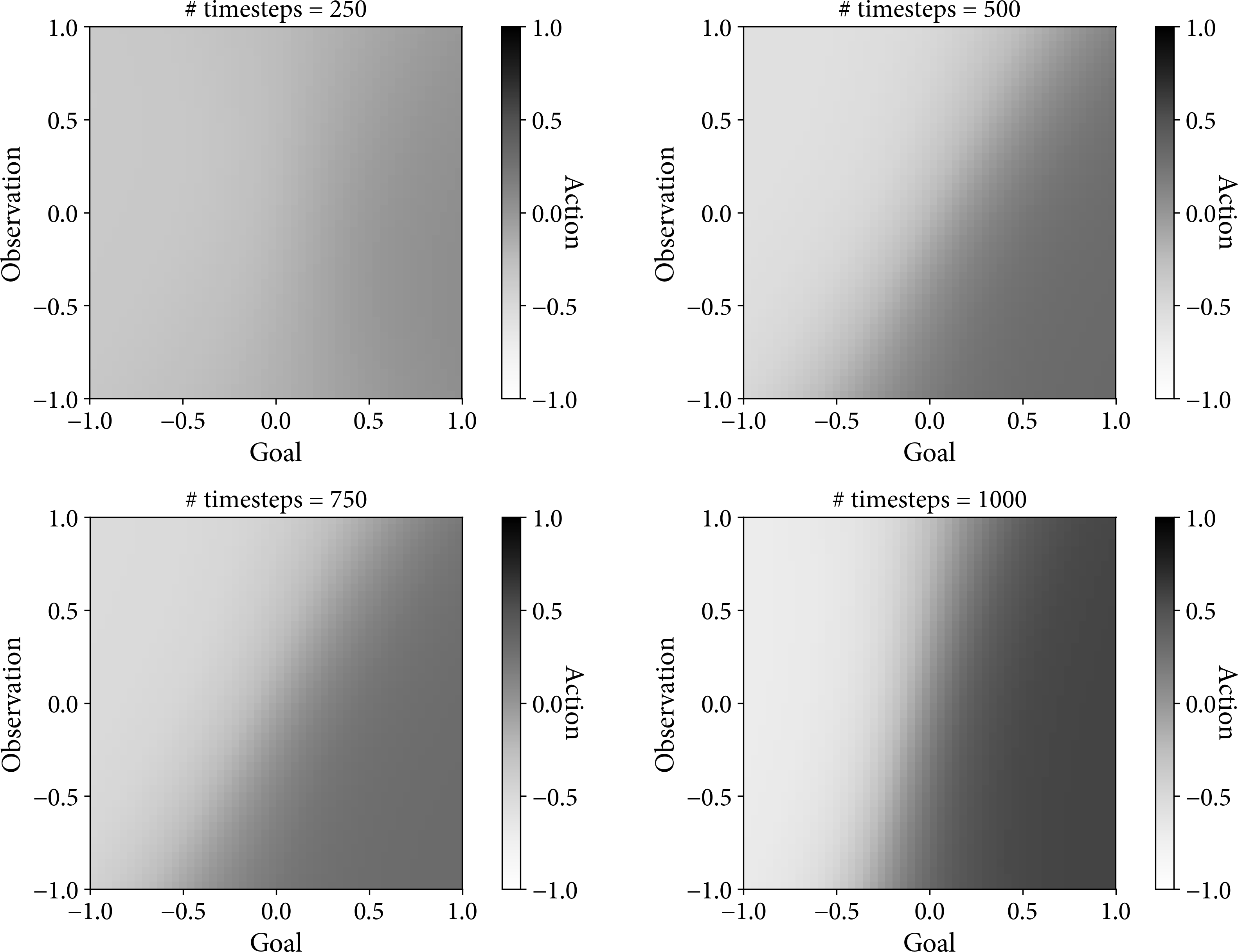
Figure 6-11. A trained policy using a real servo motor at different numbers of environment steps. Axes are the same as Figure 6-10.

Of course, like before, given more training time and averaging it would result in a perfectly viable and useful policy.

Other Policy Gradient Algorithms

Policy gradients, especially off-policy PG algorithms, are an area of enthusiastic research, because of the inherent attractiveness of directly learning a policy from experience. But in some environments, especially environments with complex state spaces, performance lags behind that of value methods. In this section I present introductions to two main streams of research: other ways of stabilizing off-policy updates, which you have already seen in the form of TRPO and PPO, and emphatic methods, which attempt to use the gradient of the Bellman error, rather than advantages.

Retrace($\lambda$)

Retrace($\lambda$) is an early off-policy PG algorithm that uses weighted and clipped importance sampling to help control how much of the off-policy is included in an update.25

Munos et al. truncate the importance sampling ratio to a maximum of 1, which is similar to the pessimistic bound in TRPO/PPO, and constrains improvements to the policy. At best the difference is minimal so the update is a standard A2C. At worst the update is negligible because the two policies are so different. The reason for clipping is to prevent variance explosion (repeated high values cause dramatic changes in the policy). The downside is that this adds bias; the result is more stable, but less able to explore.

The returns are also weighted by $\lambda$, eligibility traces from “Eligibility Traces”. This updates the policy based upon previous visitations, which provides a hyperparameter to control the bias–variance trade-off.

Actor-Critic with Experience Replay (ACER)

ACER extends Retrace($\lambda$) by including a combination of experience replay, trust region policy optimization, and a dueling network architecture.26

First, Wang et al. reformulate Retrace($\lambda$) to compensate for the bias introduced by truncating the importance sampling. To put it another way, Retrace($\lambda$) prevents large changes in policy, which makes it more stable (more biased), but less able to explore. The compensating factor compensates for this loss of exploration in proportion to the amount of truncation in Retrace($\lambda$).

They also include a more efficient TRPO implementation, which maintains an average policy, predicted by the neural network. If you code the the KL divergence as a penalty, rather than a constraint, then you can use the auto-differentiation of the DL framework.

Finally, they improve sample efficiency using experience replay (see “Experience Replay”). For continuous action spaces, they include a dueling architecture (see “Dueling Networks”) to reduce variance. This leads to two separate algorithms: one for discrete actions and one for continuous.

The result is an algorithm that approaches the performance of DQN with prioritized experience replay (see “Prioritized Experience Replay”), but can also work with continuous action spaces. However, all the corrections lead to a rather complicated algorithm and therefore a complex neural network architecture.

Actor-Critic Using Kronecker-Factored Trust Regions (ACKTR)

In “Natural Policy Gradients and Trust Region Policy Optimization” you saw that using the natural policy gradient and constraining by the KL divergence is beneficial because the gradient is independent of the parameterization of the approximating function and the KL constraint improves stability. However, calculating the gradient requires a costly computation to calculate the Fisher information matrix. TRPO’s linear projection is another source of inefficiency.

In 2017 Wu et al. proposed using approximations to speed up computation.27 They use Kronecker-factored approximation (K-FAC), which is an approximation of the Fisher information matrix, to improve computational performance, and a rolling average of this approximation instead of a linear projection, to reduce the number of times the agent has to interact with the environment.

Furthermore, because you can use K-FAC with convolutional neural networks (like PPO), this means that ACKTR can handle discrete, visual state spaces, like the Atari benchmarks.

Since 2017, independent reviews have shown that the performance of ACKTR versus TRPO is highly dependent on environment. For example, in the highly unstable Swimmer-v1 MuJoCo environment, TRPO outperforms most algorithms. But in the HalfCheetah-v1 environment, TRPO performs significantly worse.28 In the original paper, Henderson et al. present results from Swimmer-v1 that show A2C, TRPO, and ACKTR performing similarly (see “Which Algorithm Should I Use?”). Anecdotally, practitioners prefer ACKTR over TRPO because the idea and resulting performance is similar but computational efficiency is dramatically improved.

Emphatic Methods

Gradient temporal-difference methods (see “Gradient Temporal-Difference Learning”) introduced the idea using a function to approximate the state-value function and computing the gradient of the projected Bellman error directly to avoid the approximation from diverging. However, they need two sets of parameters and two learning rates, which make them hard to use in practice. To solve this, Sutton et al. proposed emphatic temporal-difference methods.^29,30

In its most general form, emphatic temporal-difference learning uses a function to quantify interest in particular states according to the current policy. This is presented alongside importance sampling to compensate for off-policy agents. However, deciding upon a function has proven difficult and performance issues relating to the projection prevent breakout success.³¹

One particularly interesting emphatic proposal called generalized off-policy actor-critic (Geoff-PAC) suggests using the gradient of a counterfactual objective.32 Counterfactual reasoning is the process of questioning data that is not observed; for example, asking what the reward of a new policy would be given data collected in the past. Although the details are beyond the scope of this book, the idea is that you can learn an approximation to the emphatic function (using a neural network of course) by predicting the density ratio, which is like a continuous version of importance sampling. The results are promising but have not gained widespread popularity.

Extensions to Policy Gradient Algorithms

Throughout this book you have seen a range of enhancements to algorithms that you could, in principle, apply to any algorithm. Every few years researchers release a paper that combines these enhancements to produce state-of-the-art results in benchmark environments and gains media attention. But from a practitioner’s point of view, it is the accompanying ablation study that tends to be more interesting, because it shows you which tweaks might be best for your problem. To demonstrate this approach, here is an example of how you can add distributional RL to PG algorithms.

Quantile Regression in Policy Gradient Algorithms

Richter et al. demonstrate how you can incorporate distributional RL into policy gradient algorithms in much the same way “Improving Rewards” did for value methods.³³ They use a neural network to predict the quantiles for each action. Like before, this is useful because the mapping from actions to rewards is often stochastic and many environments have distributions that are multimodal. The key difference in this paper is the adaption to policy gradient algorithms. They begin with the standard A2C loss function (Equation 6-8) and instead of learning the advantage function, they replace it with quantile estimates. Next they make a series of approximations to factor out the quantile estimate, which leads to a version that iteratively updates the quantile estimates according to a temperature hyperparameter. They implemented an on-policy version of this algorithm, which beat TRPO in some of the benchmarks (they didn’t compare it against PPO) and suggest that it should be possible to use this off-policy in a similar way.

Summary

In this rather extensive chapter you have seen a variety of state-of-the-art policy gradient algorithms, with a focus on off-policy actor-critic methods. Chapter 5 introduced the idea of abstracting policy evaluation and policy improvement into actor-critic architectures. The aim of this chapter was to explain and demonstrate the power of learning off-policy.

The promise of off-policy learning is great, whereby an agent learns a multitude of policies that are different from the behavior policy. Learning off-policy frees the agent from the tyranny of the exploration–exploitation trade-off, allowing the behavior policy to freely explore. Since the optimal policy is separate, you can use offline logs of data or learn from human demonstration. But the primary advantage is that you retrain your approximation functions as much as you like, because there is no environmental cost. This leads to algorithms that are far more sample-efficient, albeit at the expense of computational complexity, especially if you involve neural networks.

Which Algorithm Should I Use?

Your confusion over which algorithm is best is not lost on researchers. There have been a number of studies that have attempted to provide an answer, but to paraphrase one summary, it is very tempting for researchers to present opportunistic results that might not be entirely robust.34 To give one specific example, the original ACKTR paper presents results for a number of environments that others have struggled to reproduce. Of course, this is probably due to an implementation detail or a lucky set of hyperparameters. But it does highlight the issue. However, I can make some general recommendations:

• Prefer TD3 over DDPG

• Prefer a trust region method in environments that have unstable dynamics, which is the situation where a slight move in policy can have disastrous consequences

• Prefer deterministic methods in environments that have stable dynamics

• Consider simpler algorithms and smaller neural networks if performance or robustness is a concern, like PPO or TD3

A Note on Asynchronous Methods

Another important feature of off-policy algorithms is that it frees you from using a single critic. I haven’t mentioned it yet (see “Scaling RL”) but because the critics are learning from a replay buffer, there is no reason why you can’t have many duplicate critics all learning separate policies. In these asynchronous methods, you need to recombine that knowledge back into the behavior policy at some point, but this can dramatically improve the wall-clock performance of algorithms. I haven’t discussed it yet because I believe this is an implementation detail and depends on having a problem that needs to learn faster to justify the extra expense. For industrial problems, I would first suggest that you consider simplifying the problem or the domain to remove the need for such methods, because it adds a significant amount of operational complexity and cost.

Further Reading

• Natural policy gradients and TRPO (papers in references):

  • Brief, but nice lectures from John Schulman

  • Slides from CMU 10703

  • Lecture from Sergey Levine

  • Explanation video from Xander Steenbrugge

• Numerical optimization:

  • Nocedal, Jorge, and S. Wright. 2006. Numerical Optimization. 2nd ed. Springer Series in Operations Research and Financial Engineering. New York: Springer-Verlag.

¹ Sutton, Richard S., Hamid R. Maei, and Csaba Szepesvári. 2009. “A Convergent O(n) Temporal-Difference Algorithm for Off-Policy Learning with Linear Function Approximation”. In Advances in Neural Information Processing Systems 21, edited by D. Koller, D. Schuurmans, Y. Bengio, and L. Bottou, 1609–1616. Curran Associates, Inc.

² Sutton, Richard S., Hamid Reza Maei, Doina Precup, Shalabh Bhatnagar, David Silver, Csaba Szepesvári, and Eric Wiewiora. 2009. “Fast Gradient-Descent Methods for Temporal-Difference Learning with Linear Function Approximation”. In Proceedings of the 26th Annual International Conference on Machine Learning, 993–1000. ICML 09. Montreal, Quebec, Canada: Association for Computing Machinery.

³ Sutton, Richard S., Hamid Reza Maei, Doina Precup, Shalabh Bhatnagar, David Silver, Csaba Szepesvári, and Eric Wiewiora. 2009. “Fast Gradient-Descent Methods for Temporal-Difference Learning with Linear Function Approximation”. In Proceedings of the 26th Annual International Conference on Machine Learning, 993–1000. ICML 09. Montreal, Quebec, Canada: Association for Computing Machinery.

⁴ Maei, Hamid Reza, Csaba Szepesvári, Shalabh Bhatnagar, and Richard S. Sutton. 2010. “Toward Off-Policy Learning Control with Function Approximation.” In Proceedings of the 27th International Conference on International Conference on Machine Learning, 719–726. ICML’10. Haifa, Israel: Omnipress.

⁵ White, Adam, and Richard S. Sutton. 2017. GQ(λ) “Quick Reference and Implementation Guide”. ArXiv:1705.03967, May.

⁶ Degris, Thomas, Martha White, and Richard S. Sutton. 2013. “Off-Policy Actor-Critic”. ArXiv:1205.4839, June.

⁷ Silver, David, Guy Lever, Nicolas Heess, Thomas Degris, Daan Wierstra, and Martin Riedmiller. 2014. “Deterministic Policy Gradient Algorithms”. In International Conference on Machine Learning, 387–95.

⁸ Lillicrap, Timothy P., Jonathan J. Hunt, Alexander Pritzel, Nicolas Heess, Tom Erez, Yuval Tassa, David Silver, and Daan Wierstra. 2019. “Continuous Control with Deep Reinforcement Learning”. ArXiv:1509.02971, July.

⁹ Plappert, Matthias, Rein Houthooft, Prafulla Dhariwal, Szymon Sidor, Richard Y. Chen, Xi Chen, Tamim Asfour, Pieter Abbeel, and Marcin Andrychowicz. 2018. “Parameter Space Noise for Exploration”. ArXiv:1706.01905, January.

¹⁰ Salimans, Tim, and Durk P. Kingma. 2016. “Weight Normalization: A Simple Reparameterization to Accelerate Training of Deep Neural Networks”. In Advances in Neural Information Processing Systems 29, edited by D. D. Lee, M. Sugiyama, U. V. Luxburg, I. Guyon, and R. Garnett, 901–909. Curran Associates, Inc.

¹¹ Fujimoto, Scott, Herke van Hoof, and David Meger. 2018. “Addressing Function Approximation Error in Actor-Critic Methods”. ArXiv:1802.09477, October.

¹² Wang, Chaoyang, Zhiqiang Guo, Jianjun Li, Peng Pan, and Guohui Li. 2020. “A Text-Based Deep Reinforcement Learning Framework for Interactive Recommendation”. ArXiv:2004.06651, July.

¹³ Ie, Eugene, Vihan Jain, Jing Wang, Sanmit Narvekar, Ritesh Agarwal, Rui Wu, Heng-Tze Cheng, et al. 2019. “Reinforcement Learning for Slate-Based Recommender Systems: A Tractable Decomposition and Practical Methodology”. ArXiv:1905.12767, May.

¹⁴ Ie, Eugene, Chih-wei Hsu, Martin Mladenov, Vihan Jain, Sanmit Narvekar, Jing Wang, Rui Wu, and Craig Boutilier. 2019. “RecSim: A Configurable Simulation Platform for Recommender Systems”. ArXiv:1909.04847, September.

¹⁵ Barth-Maron, Gabriel, Matthew W. Hoffman, David Budden, Will Dabney, Dan Horgan, Dhruva TB, Alistair Muldal, Nicolas Heess, and Timothy Lillicrap. 2018. “Distributed Distributional Deterministic Policy Gradients”. ArXiv:1804.08617, April.

¹⁶ Cai, Qingpeng, Ling Pan, and Pingzhong Tang. 2019. “Deterministic Value-Policy Gradients”. ArXiv:1909.03939, November.

¹⁷ Kakade, Sham M. 2002. “A Natural Policy Gradient”. In Advances in Neural Information Processing Systems 14, edited by T. G. Dietterich, S. Becker, and Z. Ghahramani, 1531–1538. MIT Press.

¹⁸ Schulman, John, Sergey Levine, Philipp Moritz, Michael I. Jordan, and Pieter Abbeel. 2017. “Trust Region Policy Optimization”. ArXiv:1502.05477, April.

¹⁹ Peters, Jan, Sethu Vijayakumar, and Stefan Schaal. 2005. “Natural Actor-Critic”. In Machine Learning: ECML 2005, edited by João Gama, Rui Camacho, Pavel B. Brazdil, Alípio Mário Jorge, and Luís Torgo, 280–91. Lecture Notes in Computer Science. Berlin, Heidelberg: Springer.

²⁰ Schulman, John, Filip Wolski, Prafulla Dhariwal, Alec Radford, and Oleg Klimov. 2017. “Proximal Policy Optimization Algorithms”. ArXiv:1707.06347, August.

²¹ Mnih, Volodymyr, Adrià Puigdomènech Badia, Mehdi Mirza, Alex Graves, Timothy P. Lillicrap, Tim Harley, David Silver, and Koray Kavukcuoglu. 2016. “Asynchronous Methods for Deep Reinforcement Learning”. ArXiv:1602.01783, June.

²² Schulman, John, Filip Wolski, Prafulla Dhariwal, Alec Radford, and Oleg Klimov. 2017. “Proximal Policy Optimization Algorithms”. ArXiv:1707.06347, August.

²³ Ahn, Michael, Henry Zhu, Kristian Hartikainen, Hugo Ponte, Abhishek Gupta, Sergey Levine, and Vikash Kumar. 2019. “ROBEL: Robotics Benchmarks for Learning with Low-Cost Robots”. ArXiv:1909.11639, December.

²⁴ Song, Xingyou, Yilun Du, and Jacob Jackson. 2019. “An Empirical Study on Hyperparameters and Their Interdependence for RL Generalization”. ArXiv:1906.00431, June.

²⁵ Munos, Rémi, Tom Stepleton, Anna Harutyunyan, and Marc G. Bellemare. 2016. “Safe and Efficient Off-Policy Reinforcement Learning”. ArXiv:1606.02647, November.

²⁶ Wang, Ziyu, Victor Bapst, Nicolas Heess, Volodymyr Mnih, Remi Munos, Koray Kavukcuoglu, and Nando de Freitas. 2017. “Sample Efficient Actor-Critic with Experience Replay”. ArXiv:1611.01224, July.

²⁷ Wu, Yuhuai, Elman Mansimov, Shun Liao, Roger Grosse, and Jimmy Ba. 2017. “Scalable Trust-Region Method for Deep Reinforcement Learning Using Kronecker-Factored Approximation”. ArXiv:1708.05144, August.

²⁸ Henderson, Peter, Riashat Islam, Philip Bachman, Joelle Pineau, Doina Precup, and David Meger. 2019. “Deep Reinforcement Learning That Matters”. ArXiv:1709.06560, January.

²⁹ Sutton, Richard S., A. Rupam Mahmood, and Martha White. 2015. “An Emphatic Approach to the Problem of Off-Policy Temporal-Difference Learning”. ArXiv:1503.04269, April.

³⁰ Zhang, Shangtong, Wendelin Boehmer, and Shimon Whiteson. 2019. “Generalized Off-Policy Actor-Critic”. ArXiv:1903.11329, October.

³¹ Gelada, Carles, and Marc G. Bellemare. 2019. “Off-Policy Deep Reinforcement Learning by Bootstrapping the Covariate Shift”. ArXiv:1901.09455, January.

³² Zhang, Shangtong, Wendelin Boehmer, and Shimon Whiteson. 2019. “Generalized Off-Policy Actor-Critic”. ArXiv:1903.11329, October.

³³ Richter, Oliver, and Roger Wattenhofer. 2019. “Learning Policies through Quantile Regression”. ArXiv:1906.11941, September.

³⁴ Henderson, Peter, Riashat Islam, Philip Bachman, Joelle Pineau, Doina Precup, and David Meger. 2019. “Deep Reinforcement Learning That Matters”. ArXiv:1709.06560, January.