Chapter 7. Learning All Possible Policies with Entropy Methods

Deep reinforcement learning (RL) is a standard tool due to its ability to process and approximate complex observations, which result in elaborate behaviors. However, many deep RL methods optimize for a deterministic policy, since if you had full observability, there is only one best policy. But it is often desirable to learn a stochastic policy or probabilistic behaviors to improve robustness and deal with stochastic environments.

What Is Entropy?

Shannon entropy (abbreviated to entropy from now on) is a measure of the amount of information contained within a stochastic variable, where information is calculated as the number of bits required to encode all possible states. Equation 7-1 shows this as an equation where $X\doteq \{x_0,x_1,\cdots ,x_{n-1}\}$ is a stochastic variable, $\mathscr{H}$ is the entropy, $I$ is the information content, and $b$ is the base of the logarithm used (commonly bits for $b\doteq 2$, bans for $b\doteq 10$, and nats for $b\doteq e$). Bits are the most common base.

Equation 7-1. The information content of a random variable

$$\mathscr{H}\left(X\right)\doteq 𝔼\left[I\left(X\right)\right]=-\sum _{x\in X}p\left(x\right){log}_{b}p\left(x\right)$$

For example, a coin has two states, assuming it doesn’t land on its edge. These two states can be encoded by a zero and a one, therefore the amount of information contained within a coin, measured by entropy in bits, is one. A die has six possible states, so you would need three bits to describe all of those states (the real value is 2.5849…).

A probabilistic solution to optimal control is a stochastic policy. To have an accurate representation of the action-probability distribution, you must sample enough states and actions. You could measure the number of states and actions you have visited, like in UCB (see “Improving the $ϵ$-greedy Algorithm”). But this isn’t directly coupled to a policy; UCB is an exploration strategy, not part of the policy. Instead, you can use a proxy measure of how well distributed a policy is, like entropy, and include that as a penalty term in the objective function.

Maximum Entropy Reinforcement Learning

Maximizing the entropy of a policy forces the agent to visit all states and actions. Rather than aiming to find a deterministic behavior that maximizes the reward, the policy can learn all behaviors. In other words, instead of learning the best way of performing a task, the entropy term forces the agent to learn all the ways to solve a task. This leads to policies that can intuitively explore and provide more robust behavior in the face of adversarial attacks—pelting a robot with bricks, for example. See the videos on the PPO blog post for some fun. I talk more about this in Chapter 10.

Equation 7-2 shows the objective function for maximum entropy RL, where $\alpha$ is a hyperparameter (called the temperature, which links back to the thermodynamic definition of entropy) that determines the relative importance of the entropy term against the reward and controls the stochasticity of the optimal policy.

Equation 7-2. Maximum entropy objective function

$$\begin{array}{c}\hfill {\pi }^{*}\doteq \underset{\pi }{argmax}\sum _{s\in 𝒮,a\in 𝒜}𝔼\left[r+\alpha \mathscr{H}\left(\pi \right(a\mid s\left)\right)\right]\end{array}$$

Equation 7-2 states that the optimal policy is defined as the policy that maximizes the return regularized by the entropy of the policy. This is similar to the standard definition of an optimal policy except that it is augmented with a bonus to promote nondeterministic policies, the exact opposite of deterministic policy gradients.

How well this works depends on the problem. If you have a discretized problem that only has one optimal trajectory, and you never expect that the agent will veer off that trajectory, then a deterministic policy is a good choice. But in continuous problems, where it is likely that the agent will veer away from the optimal policy, then this might be a better option.

The $\alpha$ hyperparameter allows you to control how much of a bonus is included. Values close to zero become deterministic and larger values promote nondeterminate actions and therefore more exploration.

Soft Actor-Critic

The soft actor-critic (SAC) algorithm is an off-policy policy gradient approximation of the maximum entropy objective function.1 The term “soft” is used to emphasize the nondeterministic elements within the algorithm; the standard Bellman equation with no entropy term could be considered “hard,” so Q-learning and DDPG are corresponding “hard” algorithms.

Haarnoja et al. begin by defining the critic as a soft approximation of the action-value function presented in an earlier paper.² Recall that the goal is to generate a policy that maximizes the entropy, which means the agent should value high entropy states more than others. Following Equation 7-2, Equation 7-3 shows that the value of a state is the action value plus a bonus for the entropy of that new state. I have simplified the notation to match the rest of this book; Equation 7-3 assumes that you are following a policy, but I hide that information to make the mathematics easier to understand. $V$ and $Q$ represent state-value and action-value functions, respectively.

Equation 7-3. Maximum entropy state-value function

$$\begin{array}{cc}\hfill V\left(s\right)& =𝔼\left[Q(s,a)+\alpha \mathscr{H}\left(\pi (a\mid s)\right)\right]\hfill \\ & =𝔼\left[Q(s,a)-\alpha log\pi (a\mid s)\right]\hfill \end{array}$$

Using Equation 7-3, Equation 7-4 shows the corresponding action-value function from dynamic programming.

Equation 7-4. Maximum entropy action-value function

$$Q(s,a)\doteq 𝔼\left[r+\gamma 𝔼\left[V\left(s^{\text{'}}\right)\right]\right]$$

To handle complex state spaces you can train a function to approximate Equation 7-4, for which you need an objective function (Equation 7-5).

Equation 7-5. Maximum entropy action-value objective function

$$\begin{array}{cc}\hfill J_Q\left(\theta \right)& =𝔼\left[\frac{1}{2}{\left(Q_{\theta }(s,a)-Q(s,a)\right)}^2\right]\hfill \\ & =𝔼\left[\frac{1}{2}{\left(Q_{\theta }(s,a)-\left(r+\gamma 𝔼\left[V_{\theta }\left(s^{\text{'}}\right)\right]\right)\right)}^2\right]\hfill \end{array}$$

You can derive the gradient of Equation 7-4 (you will see this shortly), but SAC implementations typically leverage the automatic differential frameworks included with your deep learning library. Next, you need a policy for the actor and a similar objective function. It is possible to derive a soft policy gradient analytically.³ But Haarnoja et al. chose to minimize the Kullback–Leibler (KL) divergence instead (see “Kullback–Leibler Divergence”). The reason for this was because Liu and Wang developed an approach called Stein variational gradient descent, which is an analytical solution to the gradient of the KL divergence, the derivation of which is beyond the scope of the book.4 Haarnoja et al. applied this technique to the soft policy, which results in the policy objective shown in Equation 7-6, which you can solve using auto-differentiation.

Equation 7-6. SAC policy objective function

$$\begin{array}{c}\hfill J_{\pi }\left(\varphi \right)=𝔼\left[\alpha log\left({\pi }_{\varphi }(a\mid s)\right)-Q_{\theta }(s,a)\right]\end{array}$$

SAC Implementation Details and Discrete Action Spaces

There are details within the derivation that impact the implementation. First, performance is highly sensitive to the choice of temperature parameter. You need to perform a hyperparameter scan to establish the best temperature for each problem. Second, because of the sensitivity to the temperature hyperparameter, this also means that it is sensitive to the scale of the rewards. For example, large rewards would overwhelm small temperature values. Rescale your rewards to mitigate. These two issues are fixed in the next algorithm.

Finally, Haarnoja et al. assume Gaussian actions, which makes the problem tractable (called the reparameterization trick) and allows it to work with continuous action spaces.5 SAC does not work with discrete action spaces out of the box.

This capability is added in the SAC algorithm suggested by Christodoulou, which reformulates the maximum entropy problem with discrete actions—the differences are minimal.⁶ You might ask why use a policy gradient algorithm over something like DQN. The major benefit of using SAC with discrete action spaces is that it can compete with value methods in terms of learning performance but with zero hyperparameter tuning. SAC implements this via a subsequent algorithm that automatically adjusts the temperature.

Automatically Adjusting Temperature

A follow-up paper from Haarnoja et al. presented a way to automatically adjust the SAC temperature parameter by converting the problem into a constraint, rather than a penalty. They constrain the current policy to have a higher entropy than an expected minimum entropy of the solution. Then they find that they can iteratively update a model of the temperature parameter to minimize the difference between the entropy of the current policy and expected entropy, as shown in Equation 7-7, where $\alpha$ is the temperature parameter and $\overline{\mathscr{H}}\doteq -\text{dim}\left(𝒜\right)$ is the expected entropy, which is the same as the negative of the number of actions.⁷

Equation 7-7. SAC temperature parameter objective function

$$\begin{array}{c}\hfill J_{\alpha }=𝔼\left[-\alpha log\left(\pi (a\mid s)\right)-\alpha \overline{\mathscr{H}}\right]\end{array}$$

Haarnoja et al. add this line to the original SAC algorithm to turn it into a hyperparameter-free off-policy policy gradient algorithm. This is an enticing feature, because it mitigates against developer bias and speeds up development, with state-of-the-art performance. Of course, you still have tuning to do: neural network structure, state engineering, action class, and so on. But this is a step in the right direction.

Case Study: Automated Traffic Management to Reduce Queuing

There is nothing more universal than the synchronized groan from passengers when approaching a traffic jam. Bottlenecks generated by work zones and incidents are one of the most important contributors to nonrecurrent congestion and secondary accidents. “Smart” highways aim to improve average speed in a high-density flow by suggesting when users should merge into open lanes. Recent developments in automated driving like adaptive cruise control, which matches your speed with the vehicles in front of you, allow vehicles to drive at high speed while maintaining a small gap. But this doesn’t take advantage of knowledge of vehicles in other lanes or behind. In the future, vehicles will be able to access greater amounts of local information, which will potentially allow vehicles to collaborate. If vehicles can collaborate, then you can use RL to derive a global optimal policy to increase speed and density to reduce congestion and the number of secondary incidents.

Ren, Xie, and Jiang have developed an RL approach to solving this problem. They first split the road into zones, one of which is a merging zone where vehicles are forced to merge into an open lane. A previous zone allows for the vehicle to speed up or slow down so that they can align with traffic in an open lane.8

The state of the MDP is a velocity and acceleration matrix within this zone, and local information about the vehicle under control. This is fed into quite a complicated neural network that includes convolutional, fully connected, and recurrent elements.

The action is control over a single vehicle’s speed, in order to position it within a safe gap. They iterate over all vehicles currently within the control zone.

The reward is complex, but aims to promote successful merges (no crashes and with a safe distance) and increased speed.

They choose SAC as the algorithm of choice, because of the continuous actions, its off-policy sample efficiency, and its stability during exploration.

They simulate this formulation in a traffic simulation tool called VISSIM and compare the RL implementation to common road-sign–based merge strategies, which either tell vehicles to merge into the open lane early or late. The RL solution significantly improves mobility over the basic algorithms, reducing delays by an order of magnitude. It is also much safer, with stable, low-valued densities throughout the queue, whereas the basic algorithms promoted a dangerous backward-forming shockwave.

Despite impressive results, there is quite a lot of room for improvement. First, this is a simulation. It would have been great to have some real-life results, although I know from experience that it is incredibly difficult to develop against potentially dangerous environments such as this. I also would like to see more realistic observations. For example, vehicle position and local information can be inferred from video cameras. There is no need to assume that the vehicles or the oracle have perfect knowledge of the vehicles around them. Finally, I am concerned about the complexity of the policy model for what is quite a simple state space. I don’t believe that this much complexity is required, and that the state representation should be delegated. I’m confident the policy itself, for selecting the right speed to fit into a gap, is actually quite simple to learn.

Extensions to Maximum Entropy Methods

SAC provides you with a simple and performant off-policy algorithm out of the box but like other algorithms, researchers continue to offer improvements in the search for maximum performance. As usual, these improvements do not guarantee better performance for your specific problem; you have to test them.

Other Measures of Entropy (and Ensembles)

Shannon entropy is only one way of measuring entropy. There are other forms that alter the way SAC penalizes the policy to prefer or ignore unpromising actions. Chen and Peng try Tsallis and Rényi entropy and find that these improve performance on baseline algorithms.9 They also demonstrate the use of an ensemble of policies, whereby you train multiple policies at the same time. Upon each new episode, the agent uses a random policy from this ensemble to choose actions. This approach comes from bootstrapped DQN to improve exploration (see “Improving Exploration”).

Optimistic Exploration Using the Upper Bound of Double Q-Learning

Similar to how double Q-learning formulates a lower bound on the action-value estimate (see “Double Q-Learning”) Ciosek et al. propose using the pessimistic bound as the target policy (with an entropy term that makes it look similar to standard SAC), but the upper bound, the action value that overestimates the reward, for the behavior policy.10 They suggest that this helps prevent pessimistic under-exploration caused by relying on the lower bound. Empirically, the results on the standard MuJoCo environments are better, but not dramatically. You might want to consider this approach if you are working in an environment where agents are struggling to explore fully.

Tinkering with Experience Replay

As described in “Prioritized Experience Replay”, which experiences you choose to learn from have an impact on learning performance. Wang and Ross demonstrate that adding prioritized experience replay can improve SAC on some environments, but oversampling more recent experience improves results consistently across all environments.¹¹ This is a simple addition and worth a try, but watch out for catastrophic forgetting (see “Experience Replay”), whereby the agent forgets previous experiences. A large replay buffer mitigates against this effect.

Soft Policy Gradient

Rather than penalizing by an entropy measure, why not derive an entropy-inspired soft policy gradient instead? Shi, Song, and Wu introduced the soft policy gradient method that is reportedly more principled and stable than SAC.12

Shi et al. start by taking the maximum entropy definition of RL and differentiate the policy to result in an gradient calculation that is surprisingly simple, as shown in Equation 7-8. This is more effective than using the automatic differential frameworks because you can then observe and operate directly on the gradients, so they chose to clip the gradients directly rather than apply trust-region optimization, to prevent catastrophic updates. This results in a simpler implementation and better stability. I would not be surprised if this becomes the “default” maximum entropy interpretation in the future.

Equation 7-8. Deep soft policy gradient

$$\begin{array}{c}\hfill \nabla J_{\pi }\left(\varphi \right)=𝔼\left[\left(Q_{\theta }(s,a)-log\pi (a\mid s)-1\right){\nabla }_{\varphi }log\pi (a\mid s)\right]\end{array}$$

Soft Q-Learning (and Derivatives)

You can also apply maximum entropy RL to Q-learning. Haarnoja et al. first showed that you can derive entropy-based value and action estimates.13 Others have applied the same idea to calculate the advantage function and found it to work well on complex, potentially continuous environments that have discrete action spaces.¹⁴ I can imagine that integrating these estimates into other algorithms, like PPO, may bring positive results.

Path Consistency Learning

Path consistency learning (PCL) from Nachum et al. is related to SAC, because it appreciates that entropy encourages exploration and derives the same soft state and action value functions as soft Q-learning. However, PCL investigates using rollouts, in the style of $n$-step algorithms, and leads to an $n$-step off-policy algorithm that does not need any correction (importance sampling, for example).15 A subsequent paper implemented a KL-divergence–based trust method (Trust-PCL) that beats TRPO.16 This highlights that even with deep learning and off-policy sampling techniques, you can still incorporate improvements to the underlying temporal-difference algorithms. Despite this, SAC tends to dramatically outperform PCL methods.

Performance Comparison: SAC Versus PPO

There is an elephant in the room and it runs amok throughout RL: which algorithm is better for continuous control tasks, PPO or SAC? It is generally accepted that SAC and its derivatives perform better than PPO. But it’s not as clear as it should be. As I mentioned before, researchers measure performance in different ways and implementation details severely alter performance.17 The main issue for this section was that researchers mostly don’t publish the raw values for learning curves. And often they don’t even report values in tables, just in plots. This makes it incredibly hard to compare results between papers.

Table 7-1 shows a sample of results from papers and implementations. All results were taken at 1 million steps, except for (†) at 1.5 million steps. (*) only published images of results, so I estimated performance from the images.

Table 7-1. Performance results from continuous control benchmarks for SAC and PPO

Environment	SACa	SACb	SAC†c	SAC-auto*d	PPOe	PPO†f	SAC-autog	PPOh
MuJoCo Walker	3475	3941	3868	4800	3425	3292
MuJoCo Hopper	2101	3020	2922	3200	2316	2513
MuJoCo Half-cheetah	8896	6095	10994	11000	1669
MuJoCo Humanoid	4831		5723	5000	4900	806
MuJoCo Ant	3250	2989	3856	4100
MuJoCo Swimmer			42		111
AntBulletEnv-v0							3485	2170
BipedalWalker-v2							307	266
BipedalWalkerHardcore-v2							101	166
HalfCheetahBulletEnv-v0							3331	3195
HopperBulletEnv-v0							2438	1945
HumanoidBulletEnv-v0							2048	1286
InvertedDoublePendulumBulletEnv-v0							9357	7703
InvertedPendulumSwingupBulletEnv-v0							892	867
LunarLanderContinuous-v2							270	128
MountainCarContinuous-v0							90	92
Pendulum-v0							-160	-168
ReacherBulletEnv-v0							18	18
Walker2DBulletEnv-v0							2053	2080
a Haarnoja, Tuomas, Aurick Zhou, Pieter Abbeel, and Sergey Levine. 2018. “Soft Actor-Critic: Off-Policy Maximum Entropy Deep Reinforcement Learning with a Stochastic Actor”. ArXiv:1801.01290, August. b Wang, Tingwu, Xuchan Bao, Ignasi Clavera, Jerrick Hoang, Yeming Wen, Eric Langlois, Shunshi Zhang, Guodong Zhang, Pieter Abbeel, and Jimmy Ba. 2019. “Benchmarking Model-Based Reinforcement Learning”. ArXiv:1907.02057, July. c Wang, Che, and Keith Ross. 2019. “Boosting Soft Actor-Critic: Emphasizing Recent Experience without Forgetting the Past”. ArXiv:1906.04009, June. d Haarnoja, Tuomas, Aurick Zhou, Kristian Hartikainen, George Tucker, Sehoon Ha, Jie Tan, Vikash Kumar, et al. 2019. “Soft Actor-Critic Algorithms and Applications”. ArXiv:1812.05905, January. e Dhariwal, Prafulla, Christopher Hesse, Oleg Klimov, Alex Nichol, Matthias Plappert, Alec Radford, John Schulman, Szymon Sidor, Yuhuai Wu, and Peter Zhokhov. 2017. OpenAI Baselines. GitHub Repository. f Logan Engstrom et al. 2020. “Implementation Matters in Deep Policy Gradients: A Case Study on PPO and TRPO”. ArXiv:2005.12729, May. g Raffin, Antonin. (2018) 2020. Araffin/Rl-Baselines-Zoo. Python. https://oreil.ly/H3Nc2 h Raffin, Antonin. (2018) 2020. Araffin/Rl-Baselines-Zoo. Python. https://oreil.ly/H3Nc2

The first thing you will notice is the variance of the results. Some SAC implementations and experiments perform far worse than others. In these it is likely that worse hyperparameter tuning caused worse performance. This is why the automatic temperature variant of SAC is so important. This achieves good results without tuning. If you scan across all the numbers, then SAC mostly outperforms PPO in the MuJoCo environments. Looking at the open source PyBullet results also suggests that automatic temperature SAC is better on the whole, but there are many environments where performance is similar.

These numbers also don’t tell the whole story, though. They don’t tell you whether performance will continue to increase if you left them training. They also represent average performance; this doesn’t tell you how stable training runs were. As I have recommended several times already, always retest algorithms and implementations yourself for your specific problems. Your results might not match published baselines.

How Does Entropy Encourage Exploration?

Maximum entropy reinforcement learning encourages application, but how? Equation 7-2 added a bonus proportional to the entropy of the actions in a state, which means that the agent observes an artificial reward higher than the actual reward. The amount of extra reward is defined by the temperature value and the entropy of the actions.

Imagine a child in a candy store. You could measure candy anticipation using entropy; more choices mean more enjoyment. In the middle of the shop, the child could move in hundreds of different directions and get a new candy. But at the door, right at the edge, there’s only a few to choose from. Entropy suggests that the child would have more choices if they move toward the center of the shop.

By combining the reward with an entropy bonus you are promoting actions that are not strictly optimal. This helps to ensure that all states are adequately sampled.

To demonstrate, I created a simple grid environment with the goal in the top righthand corner and the starting point in the middle. The agent is allowed to move in any direction (including diagonals) and there is a sparse reward of one when the agent reaches the goal. The episode ends with zero reward if agents do not reach the goal within 100 steps.

I used an $ϵ$-greedy Q-learning agent as a baseline. Figure 7-1 shows the result of running the agent with action values plotted as pixels; white colors represent high action values, black low. The arrow denotes the optimal trajectory (no exploration) for the policy. You can see that it has found a path to the goal, but it is suboptimal in terms of the number of steps (remember, I am not penalizing for steps and the exploration is dependent on the random seed) and the agent hasn’t explored other regions of the state. If you changed the starting location of the agent, it would not be able to find its way to the goal. This is not a robust policy.

One simple enhancement that accounts for much of SAC’s performance is the use of the action values as a distribution, rather than relying on the random sampling of $ϵ$-greedy for exploration. When this crude probabilistic approach is applied to the Q-learning algorithm by using a softmax function to convert the action values to probabilities, exploration improves dramatically, as you can see in Figure 7-2. I also plot the most probable action as arrows for each state, of which the direction and magnitude is based upon the weighted combination of action values. Note how the direction arrows are all pointing toward the optimal trajectory, so no matter where the agent starts, it will always reach the goal. This policy is far more robust and has explored more of the state space than the previous agent.

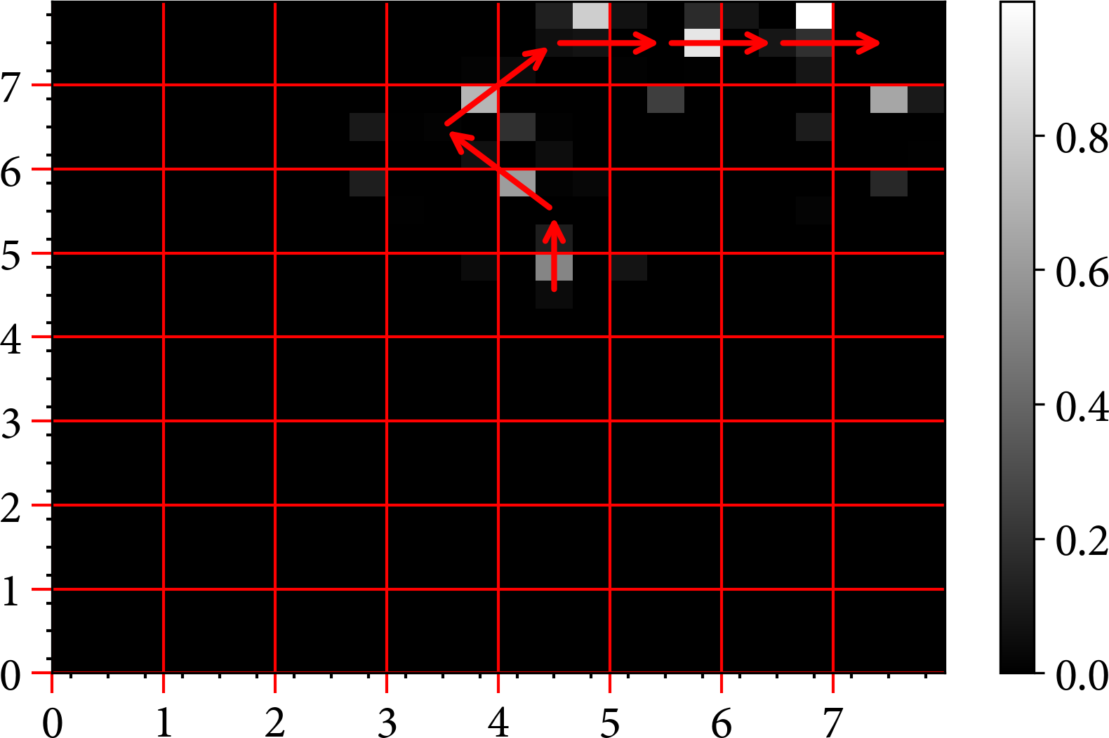
Figure 7-1. The results of using an $ϵ$-greedy Q-learning agent on a grid environment. Pixels represent action values and the grid represents the state. The arrows are the optimal trajectory according to the current policy.

Figure 7-2. The results of using a crude probabilistic, softmax-based Q-learning agent on a grid environment. Decorations are the same as Figure 7-1 except state arrows represent the most probable action with a direction and magnitude that is weighted by the action values.

Tip

The performance of a robust policy should degrade gracefully in the presence of adversity. Policies that have uncharted regions near the optimal trajectory are not robust because the tiniest of deviations could lead to states with an undefined policy.

Next I implemented soft Q-learning (see “Soft Q-Learning (and Derivatives)”) and set the temperature parameter to 0.05. You can see the results in Figure 7-3. The optimal policies are unremarkable, even though they generally point in the right direction. But if you look closely, you can see that the action values and the direction arrows are smaller or nonexistent on the Q-learning side of the plot. Soft Q-learning has visited states other than the optimal trajectory. You can also see that the white colors representing larger action values are shifted toward the center of the images for soft Q-learning. The reason is explained by the candy store example; entropy promotes states with the greatest amount of choice.

Figure 7-3. Comparing crude probabilistic Q-learning against soft Q-learning with the same setup as Figure 7-2.

The lack of exploration in the Q-learning agent is even more pronounced if you keep track of the number of times each agent visits each action, as I did in Figure 7-4. You can see that the soft Q-learning agent has sampled states more uniformly. This is why entropy helps exploration in more complex state spaces.

Figure 7-4. Number of action-value interactions for both agents. Colors represent the number of times the agent has visited each action.

How Does the Temperature Parameter Alter Exploration?

The soft Q-learning (SQL) or SAC algorithm is very dependent on the temperature parameter. It controls the amount of exploration, and if you weight entropy too highly then the agent receives higher rewards for exploration than it does for achieving the goal!

There are two solutions to this problem. The simplest is annealing. By reducing the temperature parameter over time, this forces the agent to explore early on, but become deterministic later. A second approach is to automatically learn the temperature parameter, which is used in most SAC implementations.

In the experiment in Figure 7-5 I increase the temperature value to promote more exploration. As you can see from the magnitudes of the action values, the entropy term is now so large that it overpowers the reward (with a value of 1). So the optimal policy is to move toward the states with the highest entropy, which are the states in the middle, like in the candy store.

To combat this problem, you can reduce the temperature over time to guide the child, I mean agent, toward the goal. In the experiment shown in Figure 7-6 I anneal the temperature parameter from 0.5 to 0.005. Note that the original SAC paper used annealing.

This experiment demonstrates how annealing helps the agent explore in early episodes. This is extremely useful in complex environments that require large amounts of exploration. The change in temperature causes the agent to become more Q-learning-like and homes in on the optimal policy.

Figure 7-5. Setting the temperature parameter to 1 in the soft Q-learning agent. To emphasize the effect, I increased the number of episodes to 500. All other settings are as in Figure 7-3.

Figure 7-6. Annealing the temperature parameter to from 0.5 to 0.005 in the soft Q-learning agent. All other settings are as in Figure 7-5.

However, the starting, stopping, and annealing rate parameters are important. You need to choose these carefully according to your environment and trade off robustness against optimality.

Industrial Example: Learning to Drive with a Remote Control Car

Donkey Car began life as an open source Raspberry Pi–based radio control car and made the bold move to include a single sensor; a wide-angle video camera. All of the control is derived from a single image, which poses a significant challenge and opportunity for RL. The name Donkey was chosen to set low expectations. But don’t let the name fool you; this straightforward piece of hardware is brought to life through advanced machine learning. Take a look at some of the impressive results and learn more on the Donkey Car website.

Tawn Kramer, a Donkey Car enthusiast, developed a simulation environment based upon the Unity framework.¹⁸ You can use this as a rapid development platform to develop new self-driving algorithms. And after I was inspired by Antonin Raffin, one of the core contributors to the Stable Baselines range of libraries, I decided to have a go myself.¹⁹ In this example I demonstrate that a SAC-based RL approach generates a viable policy.

Description of the Problem

The state is represented by an observation through a video camera. The video has a resolution of 160×120 with 8-bit RGB color channels. The action space is deceptively simple, allowing a throttle amount and a steering angle as input. The environment rewards the agent for speed and staying in the center of a lane/track on every time step. If the car is too far outside its lane it receives a negative reward. The goal is to reach the end of the course in the fastest time possible.

There are several tracks. The simplest is a desert road with clearly defined and consistent lanes. The hardest is an urban race simulation, where the agent has to navigate obstacles and a track without clear boundaries.

The Unity simulation is delivered as a binary. The Gym environment connects to the simulation over a websocket and supports multiple connections to allow for RL-driven competitive races.

Minimizing Training Time

Whenever you work with data that is based upon pixels, the majority of your training time will be taken up by feature extraction. The key to rapid development of a project like this is to split the problem; the more you can break it down, the faster and easier it is to improve individual components. Yes, it is possible to learn a viable policy directly from pixels, but it slows down development iterations and is costly. Your wallet will thank you.

One obvious place to start is to separate the vision part of the process. The RL agent doesn’t care if the state is a flattened image or a set of high-level features. But performance is impacted by how informative the features are; more informative features lead to faster training and more robust policies.

One computer vision approach could be to attempt to segment the image or detect the boundaries of the track. Using a perspective transformation could compensate for the forward view of the road. A segmentation algorithm or a trained segmentation model could help you pick out the road. You could use a Hough or Radon transform to find the lines in the image and use physical assumptions to find the nearest lanes. You can probably imagine more. The goal, remember, is to make the observation data more informative.

Another (or symbiotic) approach is to train an autoencoder (see “Common Neural Network Architectures”) to constrain the number of features to those that are the most informative. This consists of using a convolutional neural network that is shaped like an hourglass to decompose and reconstruct images from a dataset until the small number of neurons in the middle reliably encode all necessary information about the image. This is an offline process, independent of the RL. The pretrained low-dimensional representation is then used as the observation for RL.

Figures 7-7 and 7-8 show the original observation and reconstruction, respectively, after training a variational autoencoder for 1,000 training steps. Note how there are blurry similarities at this stage.

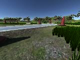
Figure 7-7. Raw observation of the DonkeyCar environment at 1,000 training steps.

Figure 7-8. Reconstruction of the DonkeyCar environment at 1,000 training steps by the variational autoencoder.

Figures 7-9 and 7-10 show another observation and reconstruction after 10,000 training steps. Note how much detail is now in the reconstruction, which indicates that the hidden neural network embedding has learned good latent features.

Figure 7-9. Raw observation of the DonkeyCar environment at 10,000 training steps.

Figure 7-10. Reconstruction of the DonkeyCar environment at 10,000 training steps by the VAE.

Figure 7-11 compares videos of the observation from the RGB camera on the Donkey Car against a reconstruction of the low-dimensional observation, which is the input to the SAC algorithm.

Figure 7-11. A reconstruction of the DonkeyCar simulation through the eyes of a variational autoencoder. The video on the left shows the raw video feed from the simulation. On the right is the reconstructed video from a low-dimensional state. This reconstructed video has been cropped to remove the sky region, which is unnecessary for this problem.

Reducing the state space, the input to the reinforcement learning algorithm, will reliably cut down RL training time to a matter of minutes, rather than days. I talk more about this in “Transformation (dimensionality reduction, autoencoders, and world models)”.

Dramatic Actions

In some environments it is possible to apply actions that dramatically alter the environment. In the case of DonkeyCar, large values for the steering action cause the car to spin, skid, and otherwise veer off the optimal trajectory. But of course, the car needs to steer and sometimes it needs to navigate around sharp corners.

But these actions and the subsequent negative rewards can cause training to get stuck, because it constantly skids and never manages to capture enough good observations. In the DonkeyCar environment, this effect becomes worse when large jumps in actions are allowed. For example, when you ride a bike, you know it is technically possible to turn the steering sharply at speed, but I doubt that you have ever tried it. You’ve probably tried something much less vigorous and had a bad experience, so you will never try anything like turning the steering by 90 degrees. Figure 7-12 shows some example training footage with the original action space.

Figure 7-12. A video of DonkeyCar training when the action space is left unaltered.

You can influence the training of the agent by including this prior information in your RL model. You could alter the reward signal to promote (or demote) certain states. Or, as in this case, you can filter the action of the agent to make it behave in a safer way.

If you try training the agent using the full range of steering angles (try it!) then you will see that after a long time it learns to steer away from the edges, but it does it so forcefully it sends the car into a three-wheel drift. Despite this looking cool, it doesn’t help finish the course. You need to smooth out the steering.

One of the simplest ways of constraining how an agent behaves is to alter the action space. Like in machine learning, constraining the problem makes it easier to solve. In the training shown in Figure 7-13 I have limited the throttle to a maximum of 0.15 (originally 5.0) and steering angle to an absolute maximum of 0.5 (originally 1.0). The slow speed prevents the car from going into a skid and the smaller steering angle helps to mitigate against the jerky steering. Note that training performance is greatly impacted by these parameters. Try altering them yourself.

Figure 7-13. A video of DonkeyCar training after simplifying the action space.

Hyperparameter Search

The maximum throttle and steering settings are hyperparameters of the problem; they are not directly tuned. Changes to the problem definition tend to impact performance the most, but there are a host of other hyperparameters from the SAC algorithm, like the architecture of the policy model. The objective is to find what combination of parameters leads to the best rewards. To do this you would perform a hyperparameter search, by writing some code that iterates through all permutations and reruns the training. You can read more about hyperparameter tuning in “Hyperparameter tuning”.

I ran an optimized grid search using the optuna library to tune the hyperparameters of the SAC algorithm and viewed all the results in TensorBoard. I found that I could increase the learning rates by an order of magnitude to speed up learning slightly. Tweaking the entropy coefficient also helped; by default the stable-baselines implementation starts with a value of 1.0 and learns the optimal value. But in this example the agent trains a small number of steps, so it doesn’t have time to learn the optimal coefficient. Starting from 0.1 and learning the optimal coefficient worked better. But overall I was underwhelmed by how much the hyperparameters affected performance (which is a good thing!). Altering the hyperparameters of the variational autoencoder and the changing the action space impacted performance much more.

Final Policy

After all the engineering work, all the code, and searching for hyperparameters, I now have a viable policy that has been trained for between 5,000 and 50,000 environment steps, depending on the environment and how perfect you want to the policy to be. This took about 10–30 minutes on my old 2014 Macbook Pro. Figures 7-14 and 7-15 show example policies for the donkey-generated-track-v0 and donkey-generated-road-v0 environments, respectively.

Figure 7-14. A video of the final DonkeyCar policy for the `donkey-generated-track-v0` environment.

Figure 7-15. A video of the final DonkeyCar policy for the `donkey-generated-road-v0` environment.

But note throughout this I barely touched upon the RL algorithm. All the hard work went into feature engineering, hyperparameter searches, and constraining the problem to make it simpler. These are precisely the tasks that take all the time in industrial ML projects. Also like ML, RL algorithms will become standardized over time, which will lead to the situation where you won’t need to touch the RL algorithms at all.

Further Improvements

You could make a multitude of improvements to this policy. By the time you read these words, other engineers will have crushed my feeble effort. You could spend your time improving the autoencoding or trying any of the other ideas suggested in “Minimizing Training Time”. You could alter the action space further, like increasing the maximum actions until it breaks. One thing I wanted to try was annealing the action space limit, whereby the action space starts small and increases up to the maximum values over training time. You could try altering the rewards, too; maybe speed shouldn’t be rewarded so highly. Attempting to penalize jerkiness makes sense, too.

You can probably imagine many more, but if you are working on an industrial problem then you will need to take more care: take baby steps, make sure you are evaluating correctly, make sure what you are doing is safe, split the problem up, constrain the problem, and test more. You can read more about this in Chapter 9.

Summary

RL aims to find a policy that maximizes the expected return from sampled states, actions, and rewards. This definition implies maximization of the expected return irrespective of the consequences. Research has shown that bounding or constraining the policy updates leads to more stable learning and better rounded policies.

Chapter 6 approached this problem by constraining updates so they don’t dramatically alter the policy. But this can still lead to brittle, overly sparse policies where most actions have zero value except for the optimal trajectory. This chapter introduced entropy-based algorithms, which modify the original definition of MDP returns to rescale or regularize the returns. This lead to proposals that other definitions of entropy might perform better, because Shannon entropy is not sparse enough. I would argue that it is possible to tweak the temperature parameter to produce a policy that suits your own problem. But it is reasonably likely that another entropy measure will perform better for your specific problem.

The logical conclusion of this argument is to use an arbitrary function. This was proposed by Li, Yang, and Zhang in regularized MDPs and mandates several theoretical rules that the function has to follow, like that it should be strictly positive, differentiable, concave, and fall to zero outside of the range of zero to one. They suggest that other exponential-based functions and trigonometric functions are interesting proposals.20

Irrespective of the implementation, augmenting the value function with an exploration bonus is a good thing for production implementations. You want your agent to be robust to change. Be careful not to overfit to your environment.

Equivalence Between Policy Gradients and Soft Q-Learning

To round this chapter off I wanted to come back to a comparison of value methods to policy methods. Simplistically, Q-learning and policy gradient methods both attempt to reinforce behavior that leads to better rewards. Q-learning increases the value of an action whereas policy gradients increase the probability of selecting an action.

When you add entropy-based policy gradients to the mix (or equivalent) you boost the probability of an action proportional to some function of the action value (refer to Equation 7-2). Or more succinctly, the policy is proportional to a function of the Q-values. Hence, policy gradient methods solve the same problem as Q-learning.²¹

Even empirically, comparisons of Q-learning and policy gradient approaches conclude that performance is similar (look at Figure 4 in the ACER paper, where policy gradient and Q-learning approaches are almost the same).²² Many of the differences can be accounted for when considering external improvements to things like sample efficiency or parallelism. Schulman and Abbeel went so far as to normalize Q-learning and policy gradient–based algorithms to be equivalent and prove they produce the same results.²³

What Does This Mean For the Future?

The conclusion you can draw from this is that given time there will be little difference between value methods and policy gradient methods. The two disciplines will merge (which they have already done to some extent with the actor-critic paradigm) since both policy improvement and value estimation are inextricably linked.

What Does This Mean Now?

But for now it is clear that no one single implementation is good for all problems, the classic interpretation of the no free lunch theorem. You have to consider several implementations to be sure that you have optimized the performance. But make sure you pick the simplest solution that solves your problem, especially if you are running this in production. The cumulative industrial knowledge and experience of these algorithms also helps. For example, you wouldn’t pick some esoteric algorithm over SAC by default, because people, platforms, and companies have more experience with SAC.

1 Haarnoja, Tuomas, Aurick Zhou, Pieter Abbeel, and Sergey Levine. 2018. “Soft Actor-Critic: Off-Policy Maximum Entropy Deep Reinforcement Learning with a Stochastic Actor”. ArXiv:1801.01290, August.

² Haarnoja, Tuomas, Haoran Tang, Pieter Abbeel, and Sergey Levine. 2017. “Reinforcement Learning with Deep Energy-Based Policies”. ArXiv:1702.08165, July.

³ Shi, Wenjie, Shiji Song, and Cheng Wu. 2019. “Soft Policy Gradient Method for Maximum Entropy Deep Reinforcement Learning”. ArXiv:1909.03198, September.

⁴ Liu, Qiang, and Dilin Wang. 2019. “Stein Variational Gradient Descent: A General Purpose Bayesian Inference Algorithm”. ArXiv:1608.04471, September.

⁵ Haarnoja, Tuomas, Aurick Zhou, Pieter Abbeel, and Sergey Levine. 2018. “Soft Actor-Critic: Off-Policy Maximum Entropy Deep Reinforcement Learning with a Stochastic Actor”. ArXiv:1801.01290, August.

⁶ Christodoulou, Petros. 2019. “Soft Actor-Critic for Discrete Action Settings”. ArXiv:1910.07207, October.

⁷ Haarnoja, Tuomas, Aurick Zhou, Kristian Hartikainen, George Tucker, Sehoon Ha, Jie Tan, Vikash Kumar, et al. 2019. “Soft Actor-Critic Algorithms and Applications”. ArXiv:1812.05905, January.

⁸ Ren, Tianzhu, Yuanchang Xie, and Liming Jiang. 2020. “Cooperative Highway Work Zone Merge Control Based on Reinforcement Learning in A Connected and Automated Environment”. ArXiv:2001.08581, January.

⁹ Chen, Gang, and Yiming Peng. 2019. “Off-Policy Actor-Critic in an Ensemble: Achieving Maximum General Entropy and Effective Environment Exploration in Deep Reinforcement Learning”. ArXiv:1902.05551, February.

¹⁰ Ciosek, Kamil, Quan Vuong, Robert Loftin, and Katja Hofmann. 2019. “Better Exploration with Optimistic Actor-Critic”. ArXiv:1910.12807, October.

¹¹ Wang, Che, and Keith Ross. 2019. “Boosting Soft Actor-Critic: Emphasizing Recent Experience without Forgetting the Past”. ArXiv:1906.04009, June.

¹² Shi, Wenjie, Shiji Song, and Cheng Wu. 2019. “Soft Policy Gradient Method for Maximum Entropy Deep Reinforcement Learning”. ArXiv:1909.03198, September.

¹³ Haarnoja, Tuomas, Haoran Tang, Pieter Abbeel, and Sergey Levine. 2017. “Reinforcement Learning with Deep Energy-Based Policies”. ArXiv:1702.08165, July.

¹⁴ “End to End Learning in Autonomous Driving Systems”. EECS at UC Berkeley. n.d. Accessed 5 May 2020.

¹⁵ Nachum, Ofir, Mohammad Norouzi, Kelvin Xu, and Dale Schuurmans. 2017. “Bridging the Gap Between Value and Policy Based Reinforcement Learning”. ArXiv:1702.08892, November.

¹⁶ Nachum, Ofir, Mohammad Norouzi, Kelvin Xu, and Dale Schuurmans. 2018. “Trust-PCL: An Off-Policy Trust Region Method for Continuous Control”. ArXiv:1707.01891, February.

¹⁷ Engstrom, Logan, Andrew Ilyas, Shibani Santurkar, Dimitris Tsipras, Firdaus Janoos, Larry Rudolph, and Aleksander Madry. 2020. “Implementation Matters in Deep Policy Gradients: A Case Study on PPO and TRPO”. ArXiv:2005.12729 Cs, Stat, May.

¹⁸ Kramer, Tawn. 2018. Tawnkramer/Gym-Donkeycar. Python.

¹⁹ Raffin, Antonin and Sokolkov, Roma. 2019. Learning to Drive Smoothly in Minutes. GitHub.

²⁰ Li, Xiang, Wenhao Yang, and Zhihua Zhang. 2019. “A Regularized Approach to Sparse Optimal Policy in Reinforcement Learning”. ArXiv:1903.00725, October.

²¹ Schulman, John, Xi Chen, and Pieter Abbeel. 2018. “Equivalence Between Policy Gradients and Soft Q-Learning”. ArXiv:1704.06440, October.

²² Mnih, Volodymyr, Adrià Puigdomènech Badia, Mehdi Mirza, Alex Graves, Timothy P. Lillicrap, Tim Harley, David Silver, and Koray Kavukcuoglu. 2016. “Asynchronous Methods for Deep Reinforcement Learning”. ArXiv:1602.01783, June.

²³ Schulman, John, Xi Chen, and Pieter Abbeel. 2018. “Equivalence Between Policy Gradients and Soft Q-Learning”. ArXiv:1704.06440, October.