5 Similarity-based Learning
When I see a bird that walks like a duck and swims like a duck and quacks like a duck, I call that bird a duck.
—James Whitcomb Riley
Similarity-based approaches to machine learning come from the idea that the best way to make a predictions is to simply look at what has worked well in the past and predict the same thing again. The fundamental concepts required to build a system based on this idea are feature spaces and measures of similarity, and these are covered in the fundamentals section of this chapter. These concepts allow us to understand the standard approach to building similarity-based models: the nearest neighbor algorithm. After covering the standard algorithm, we then look at extensions and variations that allow us to handle noisy data (the k nearest neighbor, or k-NN, algorithm), to make predictions more efficiently (k-d trees), to predict continuous targets, and to handle different kinds of descriptive features with varying measures of similarity. We also take the opportunity to introduce the use of data normalization and feature selection in the context of similarity-based learning. These techniques are generally applicable to all machine learning algorithms but are especially important when similarity-based approaches are used.
5.1 Big Idea
The year is 1798, and you are Lieutenant-Colonel David Collins of HMS Calcutta exploring the region around Hawkesbury River, in New South Wales. One day, after an expedition up the river has returned to the ship, one of the men from the expedition tells you that he saw a strange animal near the river. You ask him to describe the animal to you, and he explains that he didn’t see it very well because, as he approached it, the animal growled at him, so he didn’t approach too closely. However, he did notice that the animal had webbed feet and a duck-billed snout.
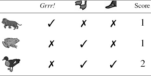
In order to plan the expedition for the next day, you decide that you need to classify the animal so that you can determine whether it is dangerous to approach it or not. You decide to do this by thinking about the animals you can remember coming across before and comparing the features of these animals with the features the sailor described to you. Table 5.1[180] illustrates this process by listing some of the animals you have encountered before and how they compare with the growling, web-footed, duck-billed animal that the sailor described. For each known animal, you count how many features it has in common with the unknown animal. At the end of this process, you decide that the unknown animal is most similar to a duck, so that is what it must be. A duck, no matter how strange, is not a dangerous animal, so you tell the men to get ready for another expedition up the river the next day.
Matching animals you remember to the features of the unknown animal described by the sailor.
Images created by Jan Gillbank, English for the Australian Curriculum website (www.e4ac.edu.au). Used under Creative Commons Attribution 3.0 license.
The process of classifying an unknown animal by matching the features of the animal against the features of animals you have encountered before neatly encapsulates the big idea underpinning similarity-based learning: if you are trying to make a prediction for a current situation then you should search your memory to find situations that are similar to the current one and make a prediction based on what was true for the most similar situation in your memory. In this chapter we are going to see how this type of reasoning can be implemented as a machine learning algorithm.
5.2 Fundamentals
As the name similarity-based learning suggests, a key component of this approach to prediction is defining a computational measure of similarity between instances. Often this measure of similarity is actually some form of distance measure. A consequence of this, and a somewhat less obvious requirement of similarity-based learning, is that if we are going to compute distances between instances, we need to have a concept of space in the representation of the domain used by our model. In this section we introduce the concept of a feature space as a representation for a training dataset and then illustrate how we can compute measures of similarity between instances in a feature space.
5.2.1 Feature Space
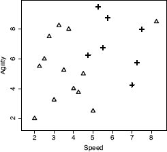
Table 5.2[182] lists an example dataset containing two descriptive features, the SPEED and AGILITY ratings for college athletes (both measures out of 10), and one target feature that lists whether the athletes were drafted to a professional team.1 We can represent this dataset in a feature space by taking each of the descriptive features to be the axes of a coordinate system. We can then place each instance within the feature space based on the values of its descriptive features. Figure 5.1[182] is a scatter plot to illustrate the resulting feature space when we do this using the data in Table 5.2[182]. In this figure SPEED has been plotted on the horizontal axis, and AGILITY has been plotted on the vertical axis. The value of the DRAFT feature is indicated by the shape representing each instance as a point in the feature space: triangles for no and crosses for yes.
There is always one dimension for every descriptive feature in a dataset. In this example, there are only two descriptive features, so the feature space is two-dimensional. Feature spaces can, however, have many more dimensions—in document classification tasks, for example, it is not uncommon to have thousands of descriptive features and therefore thousands of dimensions in the associated feature space. Although we can’t easily draw feature spaces beyond three dimensions, the ideas underpinning them remain the same.
We can formally define a feature space as an abstract m-dimensional space that is created by making each descriptive feature in a dataset an axis of an m-dimensional coordinate system and mapping each instance in the dataset to a point in this coordinate system based on the values of its descriptive features.
For similarity-based learning, the nice thing about the way feature spaces work is that if the values of the descriptive features of two or more instances in the dataset are the same, then these instances will be mapped to same point in the feature space. Also, as the differences between the values of the descriptive features of two instances grows, so too does the distance between the points in the feature space that represent these instances. So the distance between two points in the feature space is a useful measure of the similarity of the descriptive features of the two instances.
The SPEED and AGILITY ratings for 20 college athletes and whether they were drafted by a professional team.
ID |
SPEED |
AGILITY |
DRAFT |
1 |
2.50 |
6.00 |
no |
2 |
3.75 |
8.00 |
no |
3 |
2.25 |
5.50 |
no |
4 |
3.25 |
8.25 |
no |
5 |
2.75 |
7.50 |
no |
6 |
4.50 |
5.00 |
no |
7 |
3.50 |
5.25 |
no |
8 |
3.00 |
3.25 |
no |
9 |
4.00 |
4.00 |
no |
10 |
4.25 |
3.75 |
no |
11 |
2.00 |
2.00 |
no |
12 |
5.00 |
2.50 |
no |
13 |
8.25 |
8.50 |
no |
14 |
5.75 |
8.75 |
yes |
15 |
4.75 |
6.25 |
yes |
16 |
5.50 |
6.75 |
yes |
17 |
5.25 |
9.50 |
yes |
18 |
7.00 |
4.25 |
yes |
19 |
7.50 |
8.00 |
yes |
20 |
7.25 |
5.75 |
yes |
5.2.2 Measuring Similarity Using Distance Metrics
The simplest way to measure the similarity between two instances, a and b, in a dataset is to measure the distance between the instances in a feature space. We can use a distance metric to do this: metric(a, b) is a function that returns the distance between two instances a and b. Mathematically, a metric must conform to the following four criteria:
- Non-negativity: metric(a, b) ≥ 0
- Identity: metric(a, b) = 0 ⇔ a = b
- Symmetry: metric(a, b) = metric(b, a)
- Triangular Inequality: metric(a, b) ≤ metric(a, c) + metric(b, c)
One of the best known distance metrics is Euclidean distance, which computes the length of the straight line between two points. Euclidean distance between two instances a and b in an m-dimensional feature space is defined as

The descriptive features in the college athlete dataset are both continuous, which means that the feature space representing this data is technically known as a Euclidean coordinate space, and we can compute the distance between instances in it using Euclidean distance. For example, the Euclidean distance between instances d12 (SPEED = 5.00, AGILITY = 2.50) and d5 (SPEED = 2.75, AGILITY = 7.50) from Table 5.2[182] is

Another, less well-known, distance metric is the Manhattan distance.2 The Manhattan distance between two instances a and b in a feature space with m dimensions is defined as

where the abs() function returns the absolute value. For example, the Manhattan distance between instances d12 (SPEED = 5.00, AGILITY = 2.50) and d5 (SPEED = 2.75, AGILITY = 7.50) in Table 5.2[182] is

Figure 5.2(a)[184] illustrates the difference between the Manhattan and Euclidean distances between two points in a two-dimensional feature space. If we compare Equation (5.1)[183] and Equation (5.2)[183], we can see that both distance metrics are essentially functions of the differences between the values of the features. Indeed, the Euclidean and Manhattan distances are special cases of the Minkowski distance, which defines a family of distance metrics based on differences between features.
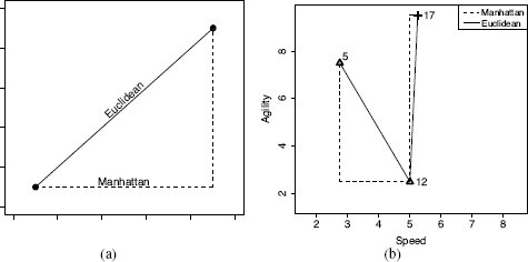
(a) A generalized illustration of the Manhattan and Euclidean distances between two points; (b) a plot of the Manhattan and Euclidean distances between instances d12 and d5 and between d12 and d17 from Table 5.2[182].
The Minkowski distance between two instances a and b in a feature space with m descriptive features is defined as

where the parameter p is typically set to a positive value and defines the behavior of the distance metric. Different distance metrics result from adjusting the value of p. For example, the Minkowski distance with p = 1 is the Manhattan distance, and with p = 2 is the Euclidean distance. Continuing in this manner, we can define an infinite number of distance metrics.
The fact that we can define an infinite number of distance metrics is not merely an academic curiosity. In fact, the predictions produced by a similarity-based model will change depending on the exact Minkowski distance used (i.e., p = 1, 2, …, ∞). Larger values of p place more emphasis on large differences between feature values than smaller values of p because all differences are raised to the power of p. Consequently, the Euclidean distance (with p = 2) is more strongly influenced by a single large difference in one feature than the Manhattan distance (with p = 1).3
We can see this if we compare the Euclidean and Manhattan distances between instances d12 and d5 with the Euclidean and Manhattan distances between instances d12 and d17 (SPEED = 5.25, AGILITY = 9.50). Figure 5.2(b)[184] plots the Manhattan and Euclidean distances between these pairs of instances.
The Manhattan distances between both pairs of instances are the same: 7.25. It is striking, however, that the Euclidean distance between d12 and d17 is 8.25, which is greater than the Euclidean distance between d12 and d5, which is just 5.48. This is because the maximum difference between d12 and d17 for any single feature is 7 units (for AGILITY), whereas the maximum difference between d12 and d5 on any single feature is just 5 units (for AGILITY). Because these differences are squared in the Euclidean distance calculation, the larger maximum single difference between d12 and d17 results in a larger overall distance being calculated for this pair of instances. Overall the Euclidean distance weights features with larger differences in values more than features with smaller differences in values. This means that the Euclidean difference is more influenced by a single large difference in one feature rather than a lot of small differences across a set of features, whereas the opposite is true of Manhattan distance.
Although we have an infinite number of Minkowski-based distance metrics to choose from, Euclidean distance and Manhattan distance are the most commonly used of these. The question of which is the best one to use, however, still remains. From a computational perspective, the Manhattan distance has a slight advantage over the Euclidean distance—the computation of the squaring and the square root is saved—and computational considerations can become important when dealing with very large datasets. Computational considerations aside, Euclidean distance is often used as the default.
5.3 Standard Approach: The Nearest Neighbor Algorithm
We now understand the two fundamental components of similarity-based learning: a feature space representation of the instances in a dataset and a measure of similarity between instances. We can put these components together to define the standard approach to similarity-based learning: the nearest neighbor algorithm. The training phase needed to build a nearest neighbor model is very simple and just involves storing all the training instances in memory. In the standard version of the algorithm, the data structure used to store training data is a simple list. In the prediction stage, when the model is used to make predictions for new query instances, the distance in the feature space between the query instance and each instance in memory is computed, and the prediction returned by the model is the target feature level of the instance that is nearest to the query in the feature space. The default distance metric used in nearest neighbor models is Euclidean distance. Algorithm 5.1[186] provides a pseudocode definition of the algorithm for the prediction stage. The algorithm really is very simple, so we can move straight to looking at a worked example of it in action.
| Algorithm 5.1 Pseudocode description of the nearest neighbor algorithm. |
| Require: a set of training instances |
Require: a query instance 1: Iterate across the instances in memory to find the nearest neighbor—this is the instance with the shortest distance across the feature space to the query instance. 2: Make a prediction for the query instance that is equal to the value of the target feature of the nearest neighbor. |
5.3.1 A Worked Example
Assume that we are using the dataset in Table 5.2[182] as our labeled training dataset, and we want to make a prediction to tell us whether a query instance with SPEED = 6.75 and AGILITY = 3.00 is likely to be drafted or not. Figure 5.3[187] illustrates the feature space of the training dataset with the query, represented by the ? marker.

A feature space plot of the data in Table 5.2[182], with the position in the feature space of the query represented by the ? marker.
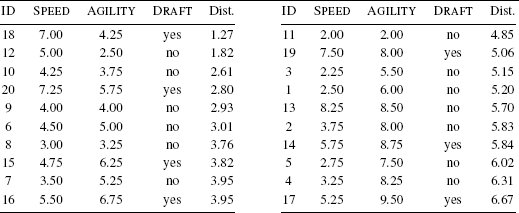
Just by visually inspecting Figure 5.3[187], we can see that the nearest neighbor to the query instance has a target level of yes, so this is the prediction that the model should return. However, let’s step through how the algorithm makes this prediction. Remember that during the prediction stage, the nearest neighbor algorithm iterates across all the instances in the training dataset and computes the distance between each instance and the query. These distances are then ranked from lowest to highest to find the nearest neighbor. Table 5.3[188] shows the distances between our query instance and each instance from Table 5.2[182] ranked from lowest to highest. Just as we saw in Figure 5.3[187], this shows that the nearest neighbor to the query is instance d18, with a distance of 1.2749 and a target level of yes.
When the algorithm is searching for the nearest neighbor using Euclidean distance, it is partitioning the feature space into what is known as a Voronoi tessellation4, and it is trying to decide which Voronoi region the query belongs to. From a prediction perspective, the Voronoi region belonging to a training instance defines the set of queries for which the prediction will be determined by that training instance. Figure 5.4(a)[189] illustrates the Voronoi tessellation of the feature space using the training instances from Table 5.2[182] and shows the position of our sample query instance within this decomposition. We can see in this figure that the query is inside a Voronoi region defined by an instance with a target level of yes. As such, the prediction for the query instance should be yes.
The distances (Dist.) between the query instance with SPEED = 6.75 and AGILITY = 3.00 and each instance in Table 5.2[182].
The nearest neighbor prediction algorithm creates a set of local models, or neighborhoods, across the feature space where each model is defined by a subset of the training dataset (in this case, one instance). Implicitly, however, the algorithm is also creating a global prediction model based on the full dataset. We can see this if we highlight the decision boundary within the feature space. The decision boundary is the boundary between regions of the feature space in which different target levels will be predicted. We can generate the decision boundary by aggregating the neighboring local models (in this case Voronoi regions) that make the same prediction. Figure 5.4(b)[189] illustrates the decision boundary within the feature space for the two target levels in the college athlete dataset. Given that the decision boundary is generated by aggregating the Voronoi regions, it is not surprising that the query is on the side of the decision boundary representing the yes target level. This illustrates that a decision boundary is a global representation of the predictions made by the local models associated with each instance in the training set. It also highlights the fact that the nearest neighbor algorithm uses multiple local models to create an implicit global model to map from the descriptive feature values to the target feature.
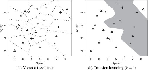
(a) The Voronoi tessellation of the feature space for the dataset in Table 5.2[182] with the position of the query represented by the ? marker; (b) the decision boundary created by aggregating the neighboring Voronoi regions that belong to the same target level.
One of the advantages of the nearest neighbor approach to prediction is that it is relatively straightforward to update the model when new labeled instances become available—we simply add them to the training dataset. Table 5.4[190] lists the updated dataset when the example query instance with its prediction of yes is included.5 Figure 5.5(a)[191] illustrates the Voronoi tessellation of the feature space that results from this update, and Figure 5.5(b)[191] presents the updated decision boundary. Comparing Figure 5.5(b)[191] with Figure 5.4(b)[189], we can see that the main difference is that the decision boundary in the bottom right region of the feature space has moved to the left. This reflects the extension of the yes region due to the inclusion of the new instance.
In summary, the inductive bias underpinning similarity-based machine learning algorithms is that things that are similar (i.e., instances that have similar descriptive features) also have the same target feature values. The nearest neighbor algorithm creates an implicit global predictive model by aggregating local models, or neighborhoods. The definition of these neighborhoods is based on similarity within the feature space to the labeled training instances. Predictions are made for a query instance using the target level of the training instance defining the neighborhood in the feature space that contains the query.
The extended version of the college athletes dataset.
ID |
SPEED |
AGILITY |
DRAFT |
1 |
2.50 |
6.00 |
no |
2 |
3.75 |
8.00 |
no |
3 |
2.25 |
5.50 |
no |
4 |
3.25 |
8.25 |
no |
5 |
2.75 |
7.50 |
no |
6 |
4.50 |
5.00 |
no |
7 |
3.50 |
5.25 |
no |
8 |
3.00 |
3.25 |
no |
9 |
4.00 |
4.00 |
no |
10 |
4.25 |
3.75 |
no |
11 |
2.00 |
2.00 |
no |
12 |
5.00 |
2.50 |
no |
13 |
8.25 |
8.50 |
no |
14 |
5.75 |
8.75 |
yes |
15 |
4.75 |
6.25 |
yes |
16 |
5.50 |
6.75 |
yes |
17 |
5.25 |
9.50 |
yes |
18 |
7.00 |
4.25 |
yes |
19 |
7.50 |
8.00 |
yes |
20 |
7.25 |
5.75 |
yes |
21 |
6.75 |
3.00 |
yes |
5.4 Extensions and Variations
We now understand the standard nearest neighbor algorithm. The algorithm, as presented, can work well with clean, reasonably sized datasets containing continuous descriptive features. Often, however, datasets are noisy, very large, and may contain a mixture of different data types. As a result, a lot of extensions and variations of the algorithm have been developed to address these issues. In this section we describe the most important of these.
5.4.1 Handling Noisy Data
Throughout our worked example using the college athlete dataset, the top right corner of the feature space contained a no region (see Figure 5.4[189]). This region exists because one of the no instances occurs far away from the rest of the instances with this target level. Considering that all the immediate neighbors of this instance are associated with the yes target level, it is likely that either this instance has been incorrectly labeled and should have a target feature value of yes, or one of the descriptive features for this instance has an incorrect value and hence it is in the wrong location in the feature space. Either way, this instance is likely to be an example of noise in the dataset.
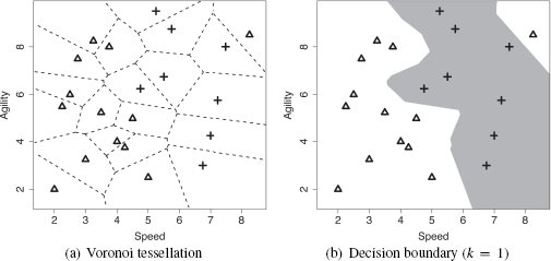
(a) The Voronoi tessellation of the feature space when the dataset has been updated to include the query instance; (b) the updated decision boundary reflecting the addition of the query instance in the training set.
Fundamentally, the nearest neighbor algorithm is a set of local models, each defined using a single instance. Consequently, the algorithm is sensitive to noise because any errors in the description or labeling of training data results in erroneous local models and hence incorrect predictions. The most direct way of mitigating against the impact of noise in the dataset on a nearest neighbor algorithm is to dilute the dependency of the algorithm on individual (possibly noisy) instances. To do this we simply modify the algorithm to return the majority target level within the set of k nearest neighbors to the query q:

where  k(q) is the prediction of the model
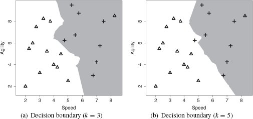
  for the query q given the parameter of the model k; levels(t) is the set of levels in the domain of the target feature, and l is an element of this set; i iterates over the instances di in increasing distance from the query q; ti is the value of the target feature for instance di; and δ(ti, l) is the Kronecker delta function, which takes two parameters and returns 1 if they are equal and 0 otherwise. Figure 5.6(a)[192] demonstrates how this approach can regularize the decision boundary for the dataset in Table 5.4[190]. In this figure we have set k = 3, and this modification has resulted in the no region in the top right corner of the feature space disappearing.
Although, in our example, increasing the set of neighbors from 1 to 3 removed the noise issue, k = 3 does not work for every dataset. There is always a trade-off in setting the value of k. If we set k too, low we run the risk of the algorithm being sensitive to noise in the data and overfitting. Conversely, if we set k too high, we run the risk of losing the true pattern of the data and underfitting. For example, Figure 5.6(b)[192] illustrates what happens to the decision boundary in our example feature space when k = 5. Here we can see that the decision boundary may have been pushed too far back into the yes region (one of the crosses is now on the wrong side of the decision boundary). So, even a small increase in k can have a significant impact on the decision boundary.
The risks associated with setting k to a high value are particularly acute when we are dealing with an imbalanced dataset. An imbalanced dataset is a dataset that contains significantly more instances of one target level than another. In these situations, as k increases, the majority target level begins to dominate the feature space. The dataset in the college athlete example is imbalanced—there are 13 no instances and only 7 yes instances. Although this differential between the target levels in the dataset may not seem substantial, it does have an impact as k increases. Figure 5.7(a)[193] illustrates the decision boundary when k = 15. Clearly, large portions of the yes region are now on the wrong side of the decision boundary. Moreover, if k is set to a value larger than 15, the majority target level dominates the entire feature space. Given the sensitivity of the algorithm to the value of k, how should we set this parameter? The most common way to tackle this issue is to perform evaluation experiments to investigate the performance of models with different values for k and to select the one that performs best. We return to these kinds of evaluation experiments in Chapter 8[397].
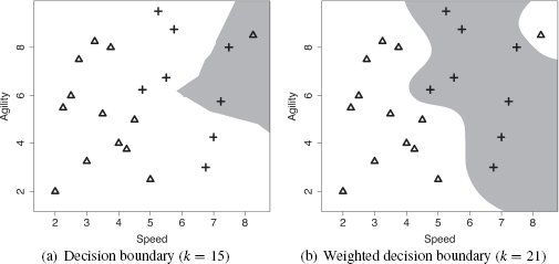
(a) The decision boundary using majority vote of the nearest 15 neighbors; (b) the weighted k nearest neighbor model decision boundary (with k = 21).
Another way to address the problem of how to set k is to use a weighted k nearest neighbor approach. The problem with setting k to a high value arises because the algorithm starts taking into account neighbors that are far away from the query instance in the feature space. As a result, the algorithm tends toward the majority target level in the dataset. One way of counterbalancing this tendency is to use a distance weighted k nearest neighbor approach. When a distance weighted k nearest neighbor approach is used, the contribution of each neighbor to the prediction is a function of the inverse distance between the neighbor and the query. So when calculating the overall majority vote across the k nearest neighbors, the votes of the neighbors that are close to the query get a lot of weight, and the votes of the neighbors that are further away from the query get less weight. The easiest way to implement this weighting scheme is to weight each neighbor by the reciprocal6 of the squared distance between the neighbor d and the query q:

Using the distance weighted k nearest neighbor approach, the prediction returned for a given query is the target level with the highest score when we sum the weights of the votes of the instances in the neighborhood of k nearest neighbors for each target level. The weighted k nearest neighbor model is defined as

where  k(q) is the prediction of the model
  for the query q given the parameter of the model k; levels(t) is the set of levels in the domain of the target feature, and l is an element of this set; i iterates over the instances di in increasing distance from the query q; ti is the value of the target feature for instance di; and δ(ti, l) is the Kronecker delta function, which takes two parameters and returns 1 if they are equal and 0 otherwise. The reason we multiply by the Kronecker delta function is to ensure that in calculating the score for each of the candidate target levels, we include only the weights for the instances whose target feature value matches that level.
When we weight the contribution to a prediction of each of the neighbors by the reciprocal of the distance to the query, we can actually set k to be equal to the size of the training set and therefore include all the training instances in the prediction process. The issue of losing the true pattern of the data is less acute now because the training instances that are very far away from the query naturally won’t have much of an effect on the prediction.
Figure 5.7(b)[193] shows the decision boundary for a weighted k nearest neighbor model for the dataset in Table 5.4[190] with k = 21 (the size of the dataset) and weights computed using the reciprocal of the squared distance. One of the most striking things about this plot is that the top-right region of the feature space again belongs to the no region. This may not be a good thing if this instance is due to noise in the data, and this demonstrates that there is no silver bullet solution to handling noise in datasets. This is one of the reasons that creating a data quality report7 and spending time on cleaning the dataset is such an important part of any machine learning project. That said, there are some other features of this plot that are encouraging. For example, the size of a no region in the top right of the feature space is smaller than the corresponding region for the nearest neighbor model with k = 1 (see Figure 5.4(b)[189]). So by giving all the instances in the dataset a weighted vote, we have a least reduced the impact of the noisy instance. Also, the decision boundary is much smoother than the decision boundaries of the other models we have looked at in this section. This may indicate that the model is doing a better job of modeling the transition between the different target levels.
Using a weighted k nearest neighbor model does not require that we set k equal to the size of the dataset, as we did in this example. It may be possible to find a value for k—using evaluation experiments—that eliminates, or further reduces, the effect of the noise on the model. As is so often the case in machine learning, fitting the parameters of a model is as important as selecting which model to use.
Finally, it is worth mentioning two situations where this weighted k nearest neighbor approach can be problematic. The first is if the dataset is very imbalanced, then even with a weighting applied to the contribution of the training instances, the majority target level may dominate. The second is when the dataset is very large, which means that computing the reciprocal of squared distance between the query and all the training instances can become too computationally expensive to be feasible.
5.4.2 Efficient Memory Search
The fact that the nearest neighbor algorithm stores the entire training dataset in memory has a negative effect on the time complexity of the algorithm. In particular, if we are working with a large dataset, the time cost in computing the distances between a query and all the training instances and retrieving the k nearest neighbors may be prohibitive. Assuming that the training set will remain relatively stable, this time issue can be offset by investing in some one-off computation to create an index of the instances that enables efficient retrieval of the nearest neighbors without doing an exhaustive search of the entire dataset.
The k-d tree,8 which is short for k-dimensional tree, is one of the best known of these indices. A k-d tree is a balanced binary tree9 in which each of the nodes in the tree (both interior and leaf nodes) index one of the instances in a training dataset. The tree is constructed so that nodes that are nearby in the tree index training instances that are nearby in the feature space.
To construct a k-d tree, we first pick a feature and split the data into two partitions using the median value of this feature.10 We then recursively split each of the two new partitions, stopping the recursion when there are fewer than two instances in a partition. The main decision to be made in this process is how to select the feature to split on. The most common way to do this is to define an arbitrary order over the descriptive features before we begin building the tree. Then, using the feature at the start of the list for the first split, we select the next feature in the list for each subsequent split. If we get to a point where we have already split on all the features, we go back to the start of the feature list.
Every time we partition the data, we add a node with two branches to the k-d tree. The node indexes the instance that had the median value of the feature, the left branch holds all the instances that had values less than the median, and the right branch holds all the instances that had values greater than the median. The recursive partitioning then grows each of these branches in a depth-first manner.
Each node in a k-d tree defines a boundary that partitions the feature space along the median value of the feature the data was split on at that node. Technically these boundaries are hyperplanes11 and, as we shall see, play an important role when we are using the k-d tree to find the nearest neighbor for a query. In particular, the hyperplane at a node defines the boundary between the instances stored on each of the subtrees below the node. We will find this useful when we are trying to decide whether to search both branches of a node when we are looking for the nearest neighbor or whether we can prune one of them.
Figure 5.8[198] illustrates the creation of the first two nodes of a k-d tree for the college athlete dataset in Table 5.4[190]. In generating this figure we have assumed that the algorithm selected the features to split on using the following ordering over the features: SPEED, AGILITY. The non-leaf nodes in the trees list the ID of the instance the node indexes and the feature and value pair that define the hyperplane partition on the feature space defined by the node. Figure 5.9(a)[199] shows the complete k-d tree generated for the dataset, and Figure 5.9(b)[199] shows the partitioning of the feature space as defined by the k-d tree. The lines in this figure indicate the hyperplanes partitioning the feature space that were created by the splits encoded in the non-leaf nodes in the tree. The heavier the weight of the line used to plot the hyperplane, the earlier in the tree the split occurred.
Once we have stored the instances in a dataset in a k-d tree, we can use the tree to quickly retrieve the nearest neighbor for a query instance. Algorithm 5.2[200] lists the algorithm we use to retrieve the nearest neighbor for a query. The algorithm starts by descending through the tree from the root node, taking the branch at each interior node that matches the value of the query for the feature tested at that node, until it comes to a leaf node (Line 3 of the algorithm). The algorithm stores the instance indexed by the leaf node in the best variable and sets the best-distance variable to the distance between the instance indexed by the leaf node and the query instance (Lines 5, 6, and 7). Unfortunately, there is no guarantee that this instance will be the nearest neighbor, although it should be a good approximate neighbor for the query. So the algorithm then searches the tree looking for instances that are closer to the query than the instance stored in best (Lines 4-11 of the algorithm control this search).
At each node encountered in the search, the algorithm does three things. First, it checks that the node is not NULL. If this is the case, then the algorithm has reached the parent node of the root of the tree and should terminate (Line 4) by returning the instance stored in best (Line 12). Second, the algorithm checks if the instance indexed by the node is closer to the query than the instance at the current best node. If it is, best and best-distance are updated to reflect this (Lines 5, 6, and 7). Third, the algorithm chooses which node it should move to next: the parent of the node or a node in the subtree under the other branch of the node (Lines 8, 9, 10, 11).
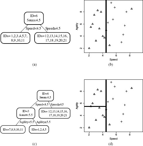
(a) The k-d tree generated for the dataset in Table 5.4[190] after the initial split using the SPEED feature with a threshold of 4.5; (b) the partitioning of the feature space by the k-d tree in (a); (c) the k-d tree after the dataset at the left child of the root has been split using the AGILITY feature with a threshold of 5.5; and (d) the partitioning of the feature space by the k-d tree in (c).
The decision of which node to move to next is made by checking if any instances indexed by nodes in the subtree on the other branch of the current node could be the nearest neighbor. The only way that this can happen is if there is at least one instance on the other side of the hyperplane boundary that bisects the node that is closer to the query than the current best-distance. Fortunately, because the hyperplanes created by the k-d tree are all axis-aligned, the algorithm can test for this condition quite easily. The hyperplane boundary bisecting a node is defined by the value used to split the descriptive feature at the node. This means that we only need to test whether the difference between the value for this feature for the query instance and the value for this feature that defines the hyperplane is less than the best-distance (Line 8). If this test succeeds, the algorithm descends to a leaf node of this subtree, using the same process it used to find the original leaf node (Line 9). If this test fails, the algorithm ascends the tree to the parent of the current node and prunes the subtree containing the region on the other side of the hyperplane without testing the instances in that region (Line 11). In either case, the search continues from the new node as before. The search finishes when it reaches the root node and both its branches have been either searched or pruned. The algorithm returns the instance stored in the best variable as the nearest neighbor.
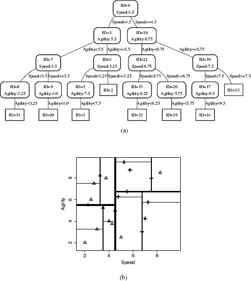
(a) The final k-d tree generated for the dataset in Table 5.4[190]; (b) the partitioning of the feature space defined by this k-d tree.
| Algorithm 5.2 Pseudocode description of the k-d tree nearest neighbor retrieval algorithm. |
Require: query instance q and a k-d tree kdtree 1: best = null 2: best-distance = ∞ 3: node = descendTree(kdtree,q) 4: while node! = NULL do 5: if distance(q,node) < best-distance then 6: best = node 7: best-distance = distance(q,node) 8: if boundaryDist(q, node) < best-distance then 9: node = descendtree(node,q) 10: else 11: node = parent(node) 12: return best |
We can demonstrate how this retrieval algorithm works by showing how the algorithm finds the nearest neighbor for a query instance with SPEED = 6.00 and AGILITY = 3.50. Figure 5.10(a)[201] illustrates the first stage of the retrieval of the nearest neighbor. The bold lines show the path taken to descend the tree from the root to a leaf node based on the values of the query instance (use Figure 5.9(a)[199] to trace this path in detail). This leaf node indexes instance d12 (SPEED = 5.00, AGILITY = 2.50). Because this is the initial descent down the tree, best is automatically set to d12, and best-distance is set to the distance between instance d12 and the query, which is 1.4142 (we use Euclidean distance throughout this example). At this point the retrieval process will have executed Lines 1–7 of the algorithm.
Figure 5.10(b)[201] illustrates the location of the query in the feature space (the ?). The dashed circle centered on the query location has a radius equal to the best-distance. We can see in Figure 5.10(b)[201] that this circle intersects with the triangle marking the location of d12, which is currently stored in best (i.e., it is our current best guess for the nearest neighbor). This circle covers the area in the feature space that we know must contain all the instances that are closer to the query than best. Although this example is just two dimensional, the k-d tree algorithm can work in a many dimensional feature space, so we will use the term target hypersphere12 to denote the region around the query that is inside the best-distance. We can see in Figure 5.10(b)[201] that instance d12 is not the true nearest neighbor to the query—several other instances are inside the target hypersphere.
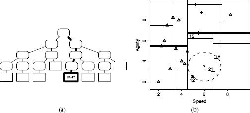
(a) The path taken from the root node to a leaf node when we search the tree with a query SPEED = 6.00, AGILITY = 3.50; (b) the ? marks the location of the query, the dashed circle plots the extent of the target, and for convenience in the discussion, we have labeled some of the nodes with the IDs of the instances they index (12, 15, 18, and 21).
The search process must now move to a new node (Lines 8, 9, 10, and 11). This move is determined by Line 8, which checks if the distance between the query and the hyperplane13 defined by the current node is less than the value of best-distance. In this case, however, the current node is a leaf node, so it does not define a hyperplane on the feature space. As a result, the condition checked in Line 8, fails and the search moves to the parent node of the current node (Line 11).
This new node indexes d15. The node is not NULL, so the while loop on Line 4 succeeds. The distance between instance d15 and the query instance is 3.0208, which is not less than the current value of best-distance, so the if statement on Line 5 will fail. We can see this easily in Figure 5.10(b)[201], as d15 is well outside the target hypersphere. The search will then move to a new node (Lines 8, 9, 10, and 11). To calculate the distance between the query instance and the hyperplane defined by the node indexing d15 (the boundaryDist function on Line 8), we use only the AGILITY feature as it is the splitting feature at this node. This distance is 2.75, which is greater than best-distance (we can see this in Figure 5.10(b)[201], as the hyperplane defined at the node indexing d15 does not intersect with the target hypersphere). This means that the if statement on Line 8 fails, and the search moves to the parent of the current node (Line 11).
This new node indexes d21, which is not NULL, so the while loop on Line 4 succeeds. The distance between the query instance and d21 is 0.9014, which is less than the value stored in best-distance (we can see this in Figure 5.10(b)[201], as d21 is inside the target hypersphere). Consequently, the if statement on Line 5 succeeds, and best is set to d21, and best-distance is set to 0.9014 (Lines 6 and 7). Figure 5.11(a)[203] illustrates the extent of the revised target hypersphere once these updates have been made.
The if statement on Line 8, which tests the distance between the query and the hyperplane defined by the current best node, is executed next. The distance between the query instance and the hyperplane defined by the node that indexes instance d21 is 0.75 (recall that because the hyperplane at this node is defined by the SPEED value of 6.75, we only compare this to the SPEED value of the query instance, 6.00). This distance is less than the current best-distance (in Figure 5.11(a)[203], the hyperplane defined by the node that indexes instance d21 intersects with the target hypersphere). The if statement on line 8 will succeed, and the search process will descend down the other branch of the current node (line 9), because there is possibly an instance closer than the current best instance stored down this branch.
It is obvious from Figure 5.11(a)[203] that the search process will not find any instances closer to the query than d21 nor are there any other hyperplanes that intersect with the target hypersphere. So the rest of the search process will involve a descent down to the node, indexing d18 and a direct ascent to the root node where the search process will then terminate and return d21 as the nearest neighbor (we will skip the details of these steps). Figure 5.11(b)[203] illustrates the parts of the k-d tree that were checked or pruned during the search process.
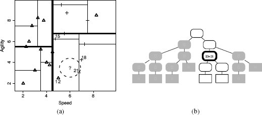
(a) The target hypersphere after instance d21 has been stored as best, and best-distance has been updated; (b) the extent of the search process: white nodes were checked by the search process, and the node with the bold outline indexed instance d21, which was returned as the nearest neighbor to the query. Grayed-out branches indicate the portions of the k-d tree pruned from the search.
In this example, using a k-d tree saved us calculating the distance between the query node and fourteen of the instances in the dataset. This is the benefit of using a k-d tree and becomes especially apparent when datasets are very large. However, using a k-d tree is not always appropriate; k-d trees are reasonably efficient when there are a lot more instances than there are features. As a rough rule of thumb, we should have around 2m instances for m descriptive features. Once this ratio drops, the efficiency of the k-d tree diminishes. Other approaches to efficient memory access have been developed, for example, locality sensitivity hashing, R-Trees, B-Trees, M-Trees, and VoRTrees among others. All these approaches are similar to k-d trees in that they are trying to set up indexes that enable efficient retrieval from a dataset. Obviously, the differences between them make them more or less appropriate for a given dataset, and it often requires some experiments to figure out which is the best one for a given problem.
We can extend this algorithm to retrieve the k nearest neighbors by modifying the search to use distance of the kth closest instance found as best-distance. We can also add instances to the tree after if has been created. This is important because one of the key advantages of a nearest neighbor approach is that it can be updated with new instances as more labeled data arrive. To add a new instance to the tree, we start at the root node and descend to a leaf node, taking the left or right branch of each node depending on whether the value of the instance’s feature is less than or greater than the splitting value used at the node. Once we get to a leaf node, we simply add the new instance as either the left or the right child of the leaf node. Unfortunately, adding nodes in this way results in the tree becoming unbalanced, which can have a detrimental effect on the efficiency of the tree. So if we add a lot of new instances, we may find that the tree has become too unbalanced and that we will need to construct a new tree from scratch using the extended dataset to restore the efficiency of the retrieval process.
A dataset listing salary and age information for customers and whether they purchased a product.
ID |
SALARY |
AGE |
PURCH |
1 |
53,700 |
41 |
no |
2 |
65,300 |
37 |
no |
3 |
48,900 |
45 |
yes |
4 |
64,800 |
49 |
yes |
5 |
44,200 |
30 |
no |
6 |
55,900 |
57 |
yes |
7 |
48,600 |
26 |
no |
8 |
72,800 |
60 |
yes |
9 |
45,300 |
34 |
no |
10 |
73,200 |
52 |
yes |
5.4.3 Data Normalization
A financial institution is planning a direct marketing campaign to sell a pension product to its customer base. In preparation for this campaign, the financial institution has decided to create a nearest neighbor model using a Euclidean distance metric to predict which customers are most likely to respond to direct marketing. This model will be used to target the marketing campaign only at those customers that are most likely to purchase the pension product. To train the model, the institution has created a dataset from the results of previous marketing campaigns that list customer information—specifically the annual salary (SALARY) and age (AGE) of the customer—and whether the customer bought a product after they had been contacted via a direct marketing message (PURCH). Table 5.5[204] lists a sample from this dataset.
Using this nearest neighbor model, the marketing department wants to decide whether they should contact a customer with the following profile:
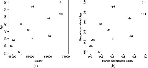
(a) The feature space defined by the SALARY and AGE features in Table 5.5[204]; (b) the normalized SALARY and AGE feature space based on the normalized data in Table 5.7[208]. The instances are labeled with their IDs; triangles represent instances with the no target level; and crosses represent instances with the yes target level. The location of the query SALARY = 56,000, AGE = 35 is indicated by the ?.
SALARY = 56,000 and AGE = 35. Figure 5.12(a)[205] presents a plot of the feature space defined by the SALARY and AGE features, containing the dataset in Table 5.5[204]. The location of the query customer in the feature space is indicated by the ?. From inspecting Figure 5.12(a)[205], it would appear as if instance d1—which has a target level no—is the closest neighbor to the query. So we would expect that the model would predict no and that the customer would not be contacted.
The model, however, will actually return a prediction of yes, indicating that the customer should be contacted. We can analyze why this happens if we examine the Euclidean distance computations between the query and the instances in the dataset. Table 5.6[207] lists these distances when we include both the SALARY and AGE features, only the SALARY features, and only the AGE feature in the distance calculation. The nearest neighbor model uses both the SALARY and AGE features when it calculates distances to find the nearest neighbor to the query. The SALARY and AGE section of Table 5.6[207] lists these distances and the ranking that the model applies to the instances in the dataset using them. From the rankings we can see that the nearest neighbor to the query is instance d6 (indicated by its rank of 1). Instance d6 has a target value of yes, and this is why the model will return a positive prediction for the query.
Considering the distribution of the instances in the feature space as depicted in Figure 5.12(a)[205], the result that instance d6 is the nearest neighbor to the query is surprising. Several other instances appear to be much closer to the query, and importantly, several of these instances have a target level of no, for example, instance d1. Why do we get this strange result?
We can get a hint about what is happening by comparing the distances computed using both the SALARY and AGE features with the distances computed using the SALARY feature only, that listed in the SALARY Only section of Table 5.6[207]. The distances calculated using only the SALARY feature are almost exactly the same as the distances calculated using both the SALARY and AGE features. This is happening because the salary values are much larger than the age values. Consequently, the SALARY feature dominates the computation of the Euclidean distance whether we include the AGE feature or not. As a result, AGE is being virtually ignored by the metric. This dominance is reflected in the ranking of the instances as neighbors. In Table 5.6[207], if we compare the rankings based on SALARY and AGE with the rankings based solely on SALARY, we see that the values in these two columns are identical. The model is using only the SALARY feature and is ignoring the AGE feature when it makes predictions.
This dominance of the distance computation by a feature based solely on the fact that it has a larger range of values than other features is not a good thing. We do not want our model to bias toward a particular feature simply because the values of that feature happen to be large relative to the other features in the dataset. If we allowed this to happen, then our model will be affected by accidental data collection factors, such as the units used to measure something. For example, in a model that is sensitive to the relative size of the feature values, a feature that was measured in millimeters would have a larger effect on the resulting model predictions than a feature that was measured in meters.14 Clearly we need to address this issue.
Fortunately, we have already discussed the solution to this problem. The problem is caused by features having different variance. In Section 3.6.1[92] we discussed variance and introduced a number of normalization techniques that normalize the variances in a set of features. The basic normalization technique we introduced was range normalization,15 and we can apply it to the pension plan prediction dataset to normalize the variance in the SALARY and AGE features. For example, range normalization using the range [0, 1] is applied to instance d1 from Table 5.5[204] as follows:

The dataset from Table 5.5[204] with the Euclidean distance between each instance and the query SALARY = 56,000, AGE = 35 when we use both the SALARY and AGE features, just the SALARY feature, and just the AGE feature.
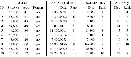
The Rank columns rank the distances of each instance to the query (1 is closest, 10 is furthest away).
Table 5.7[208] lists the dataset from Table 5.5[204] after we have applied range normalization using a range of [0, 1] to the SALARY and AGE features. When we normalize the features in a dataset, we also need to normalize the features in any query instances using the same normalization process and parameters. We normalize the query instance with SALARY =56,000 and AGE = 35 as follows:

The updated version of Table 5.6[207] once we have applied range normalization to the SALARY and AGE features in the dataset and to the query instance.
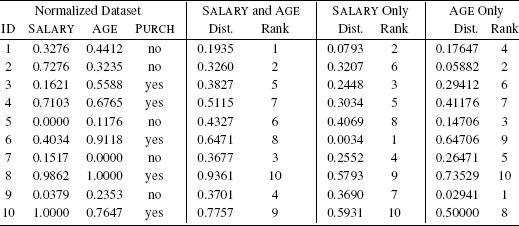
The Rank columns rank the distances of each instance to the query (1 is closest, 10 is furthest away).
Figure 5.12(b)[205] shows a plot of the feature space after the features have been normalized. The major difference between Figure 5.12(a)[205] and Figure 5.12(b)[205] is that the axes are scaled differently. In Figure 5.12(a)[205] the SALARY axis ranged from 45,000 to 75,000, and the AGE axis ranged from 25 to 60. In Figure 5.12(b)[205], however, both axes range from 0 to 1. Although this may seem like an insignificant difference, the fact that both features now cover the same range has a huge impact on the performance of a similarity-based prediction model that uses this data.
Table 5.7[208] also repeats the calculations from Table 5.6[207] using the normalized dataset and the normalized query instance. In contrast with Table 5.6[207], where there was a close match between the SALARY and AGE distances and the SALARY only distances and related rankings, in Table 5.7[208] there is much more variation between the SALARY and AGE distances and the SALARY only distances. This increased variation is mirrored in the fact that the rankings based on the distances calculated using the SALARY and AGE features are quite different from the rankings based on the distances calculated using SALARY only. These changes in the rankings of the instances is a direct result of normalizing the features and reflects the fact that the distance calculations are no longer dominated by the SALARY feature. The nearest neighbor model is now factoring both SALARY and AGE into the ranking of the instances. The net effect of this is that instance d1 is now ranked as the nearest neighbor to the query—this is in line with the feature space representation in Figure 5.12(b)[205]. Instance d1 has a target level of no, so the nearest neighbor model now predicts a target level of no for the query, meaning that the marketing department won’t include the customer in their list of direct marketing prospects. This is the opposite of the prediction made using the original dataset.
In summary, distance computations are sensitive to the value ranges of the features in the dataset. This is something we need to control for when we are creating a model, as otherwise we are allowing an unwanted bias to affect the learning process. When we normalize the features in a dataset, we control for the variation across the variances of features and ensure that each feature can contribute equally to the distance metric. Normalizing the data is an important thing to do for almost all machine learning algorithms, not just nearest neighbor.
5.4.4 Predicting Continuous Targets
It is relatively easy to adapt the k nearest neighbor approach to handle continuous target features. To do this we simply change the approach to return a prediction of the average target value of the nearest neighbors, rather than the majority target level. The prediction for a continuous target feature by a k nearest neighbor model is therefore

where  k(q) is the prediction returned by the model using parameter value k for the query q, i iterates over the k nearest neighbors to q in the dataset, and ti is the value of the target feature for instance i.
Let’s look at an example. Imagine that we are dealers in rare whiskey, and we would like some assistance in setting the reserve price for bottles of whiskey that we are selling at auction. We can use a k nearest neighbor model to predict the likely sale price of a bottle of whiskey based on the prices achieved by similar bottles at previous auctions.16 Table 5.8[210] lists a dataset of whiskeys described by the RATING they were given in popular whiskey enthusiasts magazine and their AGE (in years). The PRICE achieved at auction by the each bottle is also included.
A dataset of whiskeys listing the age (in years), the rating (between 1 and 5, with 5 being the best), and the bottle price of each whiskey.
ID |
AGE |
RATING |
PRICE |
1 |
0 |
2 |
30.00 |
2 |
12 |
3.5 |
40.00 |
3 |
10 |
4 |
55.00 |
4 |
21 |
4.5 |
550.00 |
5 |
12 |
3 |
35.00 |
6 |
15 |
3.5 |
45.00 |
7 |
16 |
4 |
70.00 |
8 |
18 |
3 |
85.00 |
9 |
18 |
3.5 |
78.00 |
10 |
16 |
3 |
75.00 |
11 |
19 |
5 |
500.00 |
12 |
6 |
4.5 |
200.00 |
13 |
8 |
3.5 |
65.00 |
14 |
22 |
4 |
120.00 |
15 |
6 |
2 |
12.00 |
16 |
8 |
4.5 |
250.00 |
17 |
10 |
2 |
18.00 |
18 |
30 |
4.5 |
450.00 |
19 |
1 |
1 |
10.00 |
20 |
4 |
3 |
30.00 |
One thing that is immediately apparent in Table 5.8[210] is that the AGE and RATING features have different ranges. We should normalize these features before we build a model. Table 5.9[211] lists the whiskey dataset after the descriptive features have been normalized, using range normalization to the range [0, 1].
Let’s now make a prediction using this model for a 2-year-old bottle of whiskey that received a magazine rating of 5. Having normalized the dataset, we first need to normalize the descriptive feature values of this query instance using the same normalization process. This results in a query with AGE = 0.0667 and RATING = 1.00. For this example we set k = 3. Figure 5.13[212] shows the neighborhood that this defines around the query instance. The three closest neighbors to the query are instances d12, d16 and d3. Consequently, the model will return a price prediction that is the average price of these three neighbors:

The whiskey dataset after the descriptive features have been normalized.
ID |
AGE |
RATING |
PRICE |
1 |
0.0000 |
0.25 |
30.00 |
2 |
0.4000 |
0.63 |
40.00 |
3 |
0.3333 |
0.75 |
55.00 |
4 |
0.7000 |
0.88 |
550.00 |
5 |
0.4000 |
0.50 |
35.00 |
6 |
0.5000 |
0.63 |
45.00 |
7 |
0.5333 |
0.75 |
70.00 |
8 |
0.6000 |
0.50 |
85.00 |
9 |
0.6000 |
0.63 |
78.00 |
10 |
0.5333 |
0.50 |
75.00 |
11 |
0.6333 |
1.00 |
500.00 |
12 |
0.2000 |
0.88 |
200.00 |
13 |
0.2667 |
0.63 |
65.00 |
14 |
0.7333 |
0.75 |
120.00 |
15 |
0.2000 |
0.25 |
12.00 |
16 |
0.2667 |
0.88 |
250.00 |
17 |
0.3333 |
0.25 |
18.00 |
18 |
1.0000 |
0.88 |
450.00 |
19 |
0.0333 |
0.00 |
10.00 |
20 |
0.1333 |
0.50 |
30.00 |
We can also use a weighted k nearest neighbor model to make predictions for continuous targets that take into account the distance from the query instance to the neighbors (just like we did for categorical target features in Section 5.4.1[190]). To do this, the model prediction equation in Equation (5.7)[209] is changed to

where dist(q, di) is the distance between the query instance and its ith nearest neighbor. This is a weighted average of the target values of the k nearest neighbors, as opposed to the simple average in Equation (5.7)[209].
Table 5.10[213] shows the calculation of the numerator and denominator of Equation (5.8)[211] for our whiskey bottle example, using the normalized dataset with k set to 20 (the full size of the dataset). The final prediction for the price of the bottle of whiskey we plan to sell is

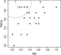
The AGE and RATING feature space for the whiskey dataset. The location of the query instance is indicated by the ? symbol. The circle plotted with a dashed line demarcates the border of the neighborhood around the query when k = 3. The three nearest neighbors to the query are labeled with their ID values.
The predictions using the k = 3 nearest neighbor model and the weighted k nearest neighbor model with k set to the size of the dataset are quite similar: 168.33 and 163.71. So, which model is making the better prediction? In this instance, to find out which model is best, we would really need to put the bottle of whiskey up for auction and see which model predicted the closest price. In situations where we have a larger dataset, however, we could perform evaluation experiments17 to see which value of k leads to the best performing model. In general, standard k nearest neighbor models and weighted k nearest neighbor models will produce very similar results when a feature space is well populated. For datasets that only sparsely populate the feature space, however, weighted k nearest neighbor models usually make more accurate predictions as they take into account the fact that some of the nearest neighbors can actually be quite far away.
5.4.5 Other Measures of Similarity
So far we have discussed and used the Minkowski-based Euclidean and Manhattan distance metrics to compute the similarity between instances in a dataset. There are, however, many other ways in which the similarity between instances can be measured. In this section we introduce some alternative measures of similarity and discuss when it is appropriate to use them. Any of these measures of similarity can simply replace the Euclidean measure we used in our demonstrations of the nearest neighbor algorithm.
The calculations for the weighted k nearest neighbor prediction.
| ID | PRICE |
Distance |
Weight |
PRICE × Weight |
| 1 | 30.00 |
0.7530 |
1.7638 |
52.92 |
| 2 | 40.00 |
0.5017 |
3.9724 |
158.90 |
| 3 | 55.00 |
0.3655 |
7.4844 |
411.64 |
| 4 | 550.00 |
0.6456 |
2.3996 |
1319.78 |
| 5 | 35.00 |
0.6009 |
2.7692 |
96.92 |
| 6 | 45.00 |
0.5731 |
3.0450 |
137.03 |
| 7 | 70.00 |
0.5294 |
3.5679 |
249.75 |
| 8 | 85.00 |
0.7311 |
1.8711 |
159.04 |
| 9 | 78.00 |
0.6520 |
2.3526 |
183.50 |
| 10 | 75.00 |
0.6839 |
2.1378 |
160.33 |
| 11 | 500.00 |
0.5667 |
3.1142 |
1557.09 |
| 12 | 200.00 |
0.1828 |
29.9376 |
5987.53 |
| 13 | 65.00 |
0.4250 |
5.5363 |
359.86 |
| 14 | 120.00 |
0.7120 |
1.9726 |
236.71 |
| 15 | 12.00 |
0.7618 |
1.7233 |
20.68 |
| 16 | 250.00 |
0.2358 |
17.9775 |
4494.38 |
| 17 | 18.00 |
0.7960 |
1.5783 |
28.41 |
| 18 | 450.00 |
0.9417 |
1.1277 |
507.48 |
| 19 | 10.00 |
1.0006 |
0.9989 |
9.99 |
| 20 | 30.00 |
0.5044 |
3.9301 |
117.90 |
Totals: |
99.2604 |
16,249.85 |
Throughout this section we use the terms similarity and distance almost interchangeably, because we often judge the similarity between two instances in terms of the distance between them in a feature space. The only difference to keep in mind is that when we use distances, smaller values mean that instances are closer together in a feature space, whereas when we use similarities, larger values indicate this. We will, however, be specific in distinguishing between metrics and indexes. Recall that in Section 5.2.2[183] we defined four criteria that a metric must satisfy: non-negativity, identity, symmetry, and triangular inequality. It is possible, however, to successfully use measures of similarity in similarity-based models that do not satisfy all four of these criteria. We refer to measures of similarity of this type as indexes. Most of the time the technical distinction between a metric and an index is not that important; we simply focus on choosing the right measure of similarity for the type of instances we are comparing. It is important, however, to know if a measure is a metric or an index as there are some similarity-based techniques that strictly require measures of similarity to be metrics. For example, the k-d trees described in Section 5.4.2[195] require that the measure of similarity used be a metric (in particular that the measure conform to the triangular inequality constraint).
5.4.5.1 Similarity Indexes for Binary Descriptive Features
There are lots of datasets that contain binary descriptive features—categorical features that have only two levels. For example, a dataset may record whether or not someone liked a movie, a customer bought a product, or someone visited a particular webpage. If the descriptive features in a dataset are binary, it is often a good idea to use a similarity index that defines similarity between instances specifically in terms of co-presence or co-absence of features, rather than an index based on distance.
To illustrate a series of similarity indexes for binary descriptive features, we will use an example of predicting upsell in an online service. A common business model for online services is to allow users a free trial period after which time they have to sign up to a paid account to continue using the service. These businesses often try to predict the likelihood that users coming to the end of the trial period will accept the upsell offer to move to the paid service. This insight into the likely future behavior of a customer can help a marketing department decide which customers coming close to the end of their trial period the department should contact to promote the benefits of signup to the paid service.
Table 5.11[215] lists a small binary dataset that a nearest neighbor model could use to make predictions for this scenario. The descriptive features in this dataset are all binary and record the following information about the behavior of past customers:
- PROFILE: Did the user complete the profile form when registering for the free trial?
- FAQ: Did the user read the frequently asked questions page?
- HELPFORUM: Did the user post a question on the help forum?
A binary dataset listing the behavior of two individuals on a website during a trial period and whether they subsequently signed up for the website.

- NEWSLETTER: Did the user sign up for the weekly newsletter?
- LIKED: Did the user Like the website on Facebook?
The target feature, SIGNUP, indicates whether the customers ultimately signed up to the paid service or not (yes or no).
The business has decided to use a nearest neighbor model to predict whether a current trial user whose free trial period is about the end is likely to sign up for the paid service. The query instance, q, describing this user is:
PROFILE = true, FAQ = false, HELPFORUM = true,NEWSLETTER = false, LIKED = false
Table 5.12[216] presents a pairwise analysis of similarity between the current trial user, q, and the two customers in the dataset in Table 5.11[215] in terms of
- co-presence (CP), how often a true value occurred for the same feature in both the query data q and the data for the comparison user (d1 or d2)
- co-absence (CA), how often a false value occurred for the same feature in both the query data q and the data for the comparison user (d1 or d2)
- presence-absence (PA), how often a true value occurred in the query data q when a false value occurred in the data for the comparison user (d1 or d2) for the same feature
- absence-presence (AP), how often a false value occurred in the query data q when a true value occurred in the data for the comparison user (d1 or d2) for the same feature
One way of judging similarity is to focus solely on co-presence. For example, in an online retail setting, co-presence could capture what two users jointly viewed, liked, or bought. The Russel-Rao similarity index focuses on this and is measured in terms of the ratio between the number of co-presences and the total number of binary features considered:

The similarity between the current trial user, q, and the two users in the dataset, d1 and d2, in terms of co-presence (CP), co-absence (CA), presence-absence (PA), and absence-presence (AP).

where q and d are two instances, |q| is the total number of features in the dataset, and CP(q, d) measures the total number of co-presences between q and d. Using Russel-Rao, q has a higher similarity to d1 than to d2:

This means that the current trial user is judged to be more similar to the customer represented by instance d1 than the customer represented by instance d2.
In some domains co-absence is important. For example, in a medical domain when judging the similarity between two patients, it may be as important to capture the fact that neither patient had a particular symptom as it is to capture the symptoms that the patients have in common. The Sokal-Michener similarity index takes this into account and is defined as the ratio between the total number of co-presences and co-absences and the total number of binary features considered:

Using Sokal-Michener for our online services example q, is judged to be more similar to instance d2 than instance d1:

Sometimes, however, co-absences aren’t that meaningful. For example, we may be in a retail domain in which there are so many items that most people haven’t seen, listened to, bought, or visited the vast majority of them, and as a result, the majority of features will be co-absences. The technical term to describe a dataset in which most of the features have zero values is sparse data. In these situations we should use a metric that ignores co-absences. The Jaccard similarity index is often used in these contexts. This index ignores co-absences and is defined as the ratio between the number of co-presences and the total number of features, excluding those that record a co-absence between a pair of instances:18

Using Jaccard similarity, the current trial user in the online retail example is judged to be equally similar to instance d1 and d2:

The fact that the judgment of similarity between current trial user and the other users in the dataset changed dramatically depending on which similarity index was employed illustrates the importance of choosing the correct index for the task. Unfortunately, beyond highlighting that the Jaccard index is useful for sparse binary data, we cannot give a hard and fast rule for how to choose between these indexes. As is so often the case in predictive analytics, making the right choice requires an understanding of the requirements of the task that we are trying to accomplish and matching these requirements with the features we want to emphasize in our model.
5.4.5.2 Cosine Similarity
Cosine similarity is an index that can be used as a measure of the similarity between instances with continuous descriptive features. The cosine similarity between two instances is the cosine of the inner angle between the two vectors that extend from the origin of a feature space to each instance. Figure 5.14(a)[220] illustrates the inner angle, θ, between the vector from the origin to two instances in a feature space defined by two descriptive features, SMS and VOICE.
Cosine similarity is an especially useful measure of similarity when the descriptive features describing instances in a dataset are related to each other. For example, in a mobile telecoms scenario, we could represent customers with just two descriptive features: the average number of SMS messages a customer sends per month, and the average number of VOICE calls a customer makes per month. In this scenario it is interesting to take a perspective on the similarity between customers that focuses on the mix of these two types of services they use, rather than the volumes of the services they use. Cosine similarity allows us to do this. The instances shown in Figure 5.14(a)[220] are based on this mobile telecoms scenario. The descriptive feature values for d1 are SMS = 97 and VOICE = 21, and for d2 are SMS = 181 and VOICE = 184.
We compute the cosine similarity between two instances as the normalized dot product of the descriptive feature values of the instances. The dot product is normalized by the product of the lengths of the descriptive feature value vectors.19 The dot product of two instances, a and b, defined by m descriptive features is

Geometrically, the dot product can be interpreted as equivalent to the cosine of the angle between the two vectors multiplied by the length of the two vectors:

We can rearrange Equation (5.13)[219] to calculate the cosine of the inner angle between two vectors as the normalized dot product:

So, in an m-dimensional feature space, the cosine similarity between two instances a and b is defined as
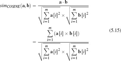
The cosine similarity between instances will be in the range [0, 1], where 1 indicates maximum similarity and 0 indicates maximum dissimilarity.20 We can calculate the cosine similarity between d1 and d2 from Figure 5.14(a)[220] as

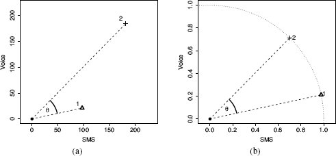
(a) The θ represents the inner angle between the vector emanating from the origin to instance d1 and the vector emanating from the origin to instance d2; (b) shows d1 and d2 normalized to the unit circle.
Figure 5.14(b)[220] highlights the normalization of descriptive feature values that takes place as part of calculating cosine similarity. This is different from the normalization we have looked at elsewhere in this chapter as it takes place within an instance rather than across all the values of a feature. All instances are normalized so as to lie on a hypersphere of radius 1.0 with its center at the origin of the feature space. This normalization is what makes cosine similarity so useful in scenarios in which we are interested in the relative spread of values across a set of descriptive features rather than the magnitudes of the values themselves. For example, if we have a third instance with SMS = 194 and VOICE = 42, the cosine similarity between this instance and d1 will be 1.0, because even though the magnitudes of their feature values are different, the relationship between the feature values for both instances is the same: both customers use about four times as many SMS messages as VOICE calls. Cosine similarity is also an appropriate similarity index for sparse data with non-binary features (i.e., datasets with lots of zero values) because the dot product will essentially ignore co-absences in its computation (0 × 0 = 0).
5.4.5.3 Mahalanobis Distance
The final measure of similarity that we will introduce is the Mahalanobis distance, which is a metric that can be used to measure the similarity between instances with continuous descriptive features. The Mahalanobis distance is different from the other distance metrics we have looked at because it allows us to take into account how spread out the instances in a dataset are when judging similarities. Figure 5.15[221] illustrates why this is important. This figure shows scatter plots for three bivariate datasets that have the same central tendency, marked A and located in the feature space at (50, 50), but whose instances are spread out differently across the feature space. In all three cases the question we would like to answer is, are instance B, located at at (30, 70), and instance C, located at (70, 70), likely to be from the same population from which the dataset has been sampled? In all three figures, B and C are equidistant from A based on Euclidean distance.

Scatter plots of three bivariate datasets with the same center point A and two queries B and C both equidistant from A; (a) a dataset uniformly spread around the center point; (b) a dataset with negative covariance; and (c) a dataset with positive covariance.
The dataset in Figure 5.15(a)[221] is equally distributed in all directions around A, and as a result, we can say that B and C are equally likely to be from the same population as the dataset. The dataset in Figure 5.15(b)[221], however, demonstrates a strong negative covariance21 between the features. In this context, instance B is much more likely to be a member of the dataset than instance C. Figure 5.15(c)[221] shows a dataset with a strong positive covariance, and for this dataset, instance C is much more likely to be a member than instance B. What these examples demonstrate is that when we are trying to decide whether a query belongs to a group, we need to consider not only the central tendency of the group, but also how spread out the members in a group are. These examples also highlight that covariance is one way of measuring the spread of a dataset.
The Mahalanobis distance uses covariance to scale distances so that distances along a direction where the dataset is very spread out are scaled down, and distances along directions where the dataset is tightly packed are scaled up. For example, in Figure 5.15(b)[221] the Mahalanobis distance between B and A will be less than the Mahalanobis distance between C and A, whereas in Figure 5.15(c)[221] the opposite will be true. The Mahalanobis distance is defined as

Let’s step through Equation (5.16)[222] bit by bit. First, this equation computes a distance between two instances a and b, each with m descriptive features. The first big term we come to in the equation is [a [1] − b [1], …, a [m] − b [m]]. This is a row vector that is created by subtracting each descriptive feature value of instance b from the corresponding feature values of a. The next term in the equation, Σ−1, represents the inverse covariance matrix22 computed across all instances in the dataset. Multiplying the difference in feature values by the inverse covariance matrix has two effects. First, the larger the variance of a feature, the less weight the difference between the values for that feature will contribute to the distance calculation. Second, the larger the correlation between two features, the less weight they contribute to the distance. The final element of the equation is a column vector that is created in the same way as the row vector at the beginning of the equation—by subtracting each feature value from b from the corresponding feature value from a. The motivation for using a row vector to hold one copy of the feature differences and a column vector to hold the second copy of the features differences is to facilitate matrix multiplication. Now that we know that the row and column vector both contain the difference between the feature values of the two instances, it should be clear that, similar to Euclidean distance, the Mahalanobis distance squares the differences of the features. The Mahalanobis distance, however, also rescales the differences between feature values (using the inverse covariance matrix) so that all the features have unit variance, and the effects of covariance are removed.
The Mahalanobis distance can be understood as defining an orthonormal coordinate system with (1) an origin at the instance we are calculating the distance from (a in Equation (5.16)[222]); (2) a primary axis aligned with the direction of the greatest spread in the dataset; and (3) the units of all the axes scaled so that the dataset has unit variance along each axis. The rotation and scaling of the axes are the result of the multiplication by the inverse covariance matrix of the dataset (Σ−1). So, if the inverse covariance matrix is the identity matrix  , then no scaling or rotation occurs. This is why for datasets such as the one depicted in Figure 5.15(a)[221], where there is no covariance between the features, the Mahalanobis distance is simply the Euclidean distance.23
Figure 5.16[224] illustrates how the Mahalanobis distance defines this coordinate system, which is translated, rotated, and scaled with respect to the standard coordinates of a feature space. The three scatter plots in this image are of the dataset in Figure 5.15(c)[221]. In each case we have overlaid the coordinate system defined by the Mahalanobis distance from a different origin. The origins used for the figures were (a) (50, 50), (b) (63, 71), and (c) (42, 35). The dashed lines plot the axes of the coordinate system, and the ellipses plot the 1, 3, and 5 unit distance contours. Notice how the orientation of the axes and the scaling of the distance contours are consistent across the figures. This is because the same inverse covariance matrix based on the entire dataset was used in each case.
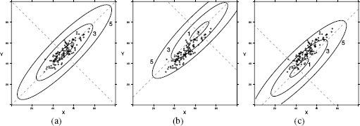
The coordinate systems defined by the Mahalanobis distance using the co-variance matrix for the dataset in Figure 5.15(c)[221] using three different origins: (a) (50, 50), (b) (63, 71), (c) (42, 35). The ellipses in each figure plot the 1, 3, and 5 unit distance contours.
Let’s return to the original question depicted in Figure 5.15[221]: Are B and C likely to be from the same population from which the dataset has been sampled? Focusing on Figure 5.15(c)[221], for this dataset it appears reasonable to conclude that instance C is a member of the dataset but that B is probably not. To confirm this intuition we can calculate the Mahalanobis distance between A and B and A and C using Equation (5.16)[222] as
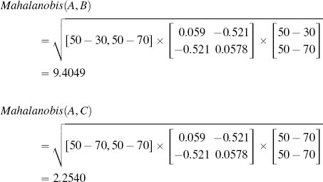
where the inverse covariance matrix used in the calculations is based on the covariance matrix24 calculated directly from the dataset: 
Figure 5.17[225] shows a contour plot of these Mahalanobis distances. In this figure, A indicates the central tendency of the dataset in Figure 5.15(c)[221], and the ellipses plot the Mahalanobis distance contours that the distances from A to the instances B and C lie on. These distance contours were calculated using the inverse covariance matrix for the dataset and point A as the origin. The result is that instance C is much closer to A than B and so should be considered a member of the same population as this dataset.
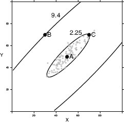
The effect of using a Mahalanobis versus Euclidean distance. A marks the central tendency of the dataset in Figure 5.15(c)[221]. The ellipses plot the Mahalanobis distance contours from A that B and C lie on. In Euclidean terms, B and C are equidistant from A; however, using the Mahalanobis distance, C is much closer to A than B.
To use Mahalanobis distance in a nearest neighbor model, we simply use the model in exactly the same way as described previously but substitute Mahalanobis distance for Euclidean distance.
5.4.5.4 Summary
In this section we have introduced a number of commonly used metrics and indexes for judging similarity between instances in a feature space. These are typically used in situations where a Minkowski distance is not appropriate. For example, if we are dealing with binary features, it may be more appropriate to use the Russel-Rao, Sokal-Michener or Jaccard similarity metric. Or it may be that the features in the dataset are continuous—typically indicating that a Minkowski distance metric is appropriate—but that the majority of the descriptive features for each instance have zero values,25 in which case we may want to use a similarity index that ignores descriptive features with zero values in both features, for example, cosine similarity. Alternatively, we may be dealing with a dataset where there is covariance between the descriptive features, in which case we should consider using the Mahalanobis distance as our measure of similarity. There are many other indexes and metrics we could have presented, for example, Tanimoto similarity (which is a generalization of the Jaccard similarity to non-binary data), and correlation-based approaches such as the Pearson correlation. The key things to remember, however, are that it is important to choose a similarity metric or index that is appropriate for the properties of the dataset we are using (be it binary, non-binary, sparse, covariant, etc.) and second, experimentation is always required to determine which measure of similarity will be most effective for a specific prediction model.
5.4.6 Feature Selection
Intuitively, adding more descriptive features to a dataset provides more information about each instance and should result in more accurate predictive models. Surprisingly, however, the number of descriptive features in a dataset increases, there often comes a point at which continuing to add new features to the dataset results in a decrease in the predictive power of the induced models. The reason for this phenomenon is that, fundamentally, the predictive power of an induced model is based on one of the following:
- Partitioning the feature space into regions based on clusters of training instances with the same target value, and assigning a query located in a region the target value of the cluster that defines that region.
- Assigning a query a target value interpolated (for instance, by majority vote or average) from the target values of individual training instances that are near the query in the feature space.
Both of these strategies depend on a reasonable sampling density of the training instances across the feature space. The sampling density is the average density of training instances across the feature space. If the sampling density is too low, then large regions of the feature space do not contain any training instances, and it doesn’t make sense to associate such a region with any cluster of training instances nor to look for training instances that are nearby. In such instances a model is essentially reduced to guessing predictions. We can measure the sampling density across a feature space in terms of the average density of a unit hypercube26 in the feature space. The density of a unit hypercube is equal to

where k is the number of instances inside the hypercube, and m is the number of dimensions of the feature space.
Figure 5.18[229] provides a graphical insight into the relationship between the number of descriptive features in a dataset and the sampling density of the feature space. Figure 5.18(a)[229] plots a one-dimensional dataset consisting of 29 instances spread evenly between 0.0 and 3.0. We have marked the unit hypercube covering the interval 0 to 1 in this figure. The density of this unit hypercube is  (there are 10 instances inside the hypercube). If we increase the number of descriptive features, the dimensionality of the feature space increases. Figures 5.18(b)[229] and 5.18(c)[229] illustrate what happens if we increase the number of descriptive features in a dataset but do not increase the number of instances. In Figure 5.18(b)[229] we have added a second descriptive feature, Y, and assigned each of the instances in the dataset a random Y value in the range [0.0, 3.0]. The instances have moved away from each other, and the sampling density has decreased. The density of the marked unit hypercube is now
  (there are only 4 instances inside the hypercube). Figure 5.18(c)[229] illustrates the distribution of the original 29 instances when we move to a three-dimensional feature space (each instance has been given a random value in the range [0.0, 3.0] for the Z feature). It is evident that the instances are getting farther and farther away from each other, and the feature space is becoming very sparsely populated, with relatively large areas where there are no or very few instances. This is reflected in a further decrease in the sampling density. The density of the marked hypercube is
Figures 5.18(d)[229] and 5.18(e)[229] illustrate the cost we would have to incur in extra instances if we wished to maintain the sampling density in the dataset in line with each increase in the dimensionality of the feature space. In the two-dimensional feature space in Figure 5.18(d)[229], we have maintained the sampling density (the density of the marked unit hypercube is  ) at the expense of a very large increase in the number of instances—there are 29 × 29 = 841 instances plotted in this figure. This is quite a dramatic increase; however, it gets even more dramatic when we increase from two to three descriptive features. In Figure 5.18(e)[229] we have, again, maintained the sampling density (the density of the marked unit hypercube is
  ) at the expense of a very large increase in the number of instances—there are 29 × 29 × 29 = 24,389 instances in this figure!
So, in order to maintain the sampling density of the feature space as the number of descriptive features increases, we need to dramatically, indeed exponentially, increase the number of instances. If we do not do this, then as we continue to increase the dimensionality of the feature space, the instances will continue to spread out until we reach a point in a high-dimensional feature space where most of the feature space is empty. When this happens, most of the queries will be in locations where none of the training instances are nearby, and as a result, the predictive power of the models based on these training instances will begin to decrease. This trade-off between the number of descriptive features and the density of the instances in the feature space is known as the curse of dimensionality.
Typically, we are not able to increase the number of instances in our dataset, and we face the scenario of a sparsely populated feature space,27 as illustrated in Figures 5.18(b)[229] and 5.18(c)[229]. Fortunately, several features of real data can help us to induce reasonable models in high-dimensional feature spaces.28 First, although real data does spread out, it doesn’t spread out quite as randomly and quickly as we have illustrated here. Real instances tend to cluster. The net effect of this is that the distribution of real data tends to have a lower effective dimensionality than the dimensionality of the feature space. Second, within any small region or neighborhood of the feature space, real data tends to manifest a smooth correlation between changes in descriptive feature values and the values of the target feature. In other words, small changes in descriptive features result in small changes in the target feature. This means that we can generate good predictions for queries by interpolating from nearby instances with known target values.
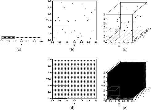
A set of scatter plots illustrating the curse of dimensionality. Across (a), (b), and (c), the number of instances remains the same, so the density of the marked unit hypercubes decreases as the number of dimensions increases; (d) and (e) illustrate the cost we must incur, in terms of the number of extra instances required, if we wish to maintain the density of the instances in the feature space as its dimensionality increases.
Another factor that can help us deal with the curse of dimensionality is that some learning algorithms have a natural resistance to the problem. For example, the decision tree learning algorithms we looked at in the last chapter worked by selecting subsets of features from which to build predictive trees and so naturally reduce dimensionality. Even these algorithms, however, do eventually succumb to the curse as the dimensionality grows. Other algorithms, such as the nearest neighbor algorithm, that use all the descriptive features when making a prediction are particularly sensitive to the curse. The moral here is that the curse of dimensionality is a problem for all inductive learning approaches, and given that acquiring new labeled instances is typically not an option, the best way to avoid it is to restrict the number of descriptive features in a dataset to the smallest set possible, while still providing the learning algorithm with enough information about the instances to be able to build a useful model. This is difficult, however, because when we design descriptive features, we tend not to know exactly which ones will be predictive and which ones will not.
Fortunately, we can use feature selection29 to help reduce the number of descriptive features in a dataset to just the subset that is most useful. Before we begin our discussion of approaches to feature selection, it is useful to distinguish between different types of descriptive features.
- Predictive: a predictive descriptive feature provides information that is useful in estimating the correct value of a target feature.
- Interacting: by itself, an interacting descriptive feature is not informative about the value of the target feature. In conjunction with one or more other features, however, it becomes informative.
- Redundant: a descriptive feature is redundant if it has a strong correlation with another descriptive feature.
- Irrelevant: an irrelevant descriptive feature does not provide information that is useful in estimating the value of the target feature.
The goal of any feature selection approach is to identify the smallest subset of descriptive features that maintains overall model performance. Ideally, a feature selection approach will return the subset of features that includes the predictive and interacting features while excluding the irrelevant and redundant features.
The most popular and straight forward approach to feature selection is to rank and prune. In this approach the features are ranked using a measure of their predictiveness, and any feature outside the top X% of the features in the list is pruned. The measures of predictiveness are called filters because they are used to filter apparently irrelevant features before learning occurs. Technically, a filter can be defined as a heuristic rule that assesses the predictiveness of a feature using only the intrinsic properties of the data, independently of the learning algorithm that will use the features to induce the model. For example, we can use information gain30 as a filter in a rank and prune approach.
Although rank and prune approaches using filters are computationally efficient, they suffer from the fact that the predictiveness of each feature is evaluated in isolation from the other features in the dataset. This leads to the undesirable result that ranking and pruning can exclude interacting features and include redundant features.
To find the ideal subset of descriptive features to use to train a model, we could attempt to build a model using every possible subset, evaluate the performance of all these models, and select the feature subset that leads to the best model. This is unfeasible, however, as for d features, there are 2d different possible feature subsets, which is far too many to evaluate unless d is very small. For example, with just 20 descriptive features, there are 220 = 1,048,576 possible feature subsets. Instead, feature selection algorithms often frame feature selection as a greedy local search problem, where each state in the search space specifies a subset of possible features. For example, Figure 5.19[232] illustrates a feature subset space for a dataset with three descriptive features: X, Y, and Z. In this figure each rectangle represents a state in the search space that is a particular feature subset. For instance, the rectangle on the very left represents the feature subset that includes no features at all, and the rectangle at the top of the second column from the left represents the feature subset including just the feature X. Each state is connected to all the other states that can be generated by adding or removing a single feature from that state. A greedy local search process moves across a feature subset space like this search in order to find the best feature subset.
When framed as a greedy local search problem, feature selection is defined in terms of an iterative process consisting of the following components:
- Subset Generation: This component generates a set of candidate feature subsets that are successors of the current best feature subset.
- Subset Selection: This component selects the feature subset from the set of candidate feature subsets generated by the subset generation component that is the most desirable for the search process to move to. One way to do this (similar to the ranking and pruning approach described previously) is to use a filter to evaluate the predictiveness of each candidate set of features and select the most predictive one. A more common approach is to use a wrapper. A wrapper evaluates a feature subset in terms of the potential performance of the models that can be induced using that subset. This involves performing an evaluation experiment31 for each candidate feature subset, in which a model is induced using only the features in the subset, and its performance is evaluated. The candidate feature subset that leads to the best performing model is then selected. Wrapper approaches are more computationally expensive than filters, as they involve training multiple models during each iteration. The argument for using a wrapper approach is that to get the best predictive accuracy, the inductive bias of the particular machine learning algorithm that will be used should be taken into consideration during feature selection. That said, filter approaches are faster and often result in models with good accuracy.
- Termination Condition: This component determines when the search process should stop. Typically we stop when the subset selection component indicates that none of the feature subsets (search states) that can be generated from the current feature subset is more desirable than the current subset. Once the search process is terminated, the features in the dataset that are not members of the selected feature subset are pruned from the dataset before the prediction model is induced.
Forward sequential selection is a commonly used implementation of the greedy local search approach to feature selection. In forward sequential selection, the search starts in a state with no features (shown on the left of Figure 5.19[232]). In the subset generation component of forward sequential selection, the successors of the current best feature subset are the set of feature subsets that can be generated from the current best subset by adding just a single extra feature. For example, after beginning with the feature subset including no features, the forward sequential search process generates three feature subsets, each containing just one of X, Y, or Z (shown in the second column of Figure 5.19[232]). The subset selection component in forward sequential selection can use any of the approaches described above and moves the search process to a new feature subset. For example, after starting with the feature subset including no features, the process will move to the most desirable of the feature subsets containing just one feature. Forward sequential selection terminates when no accessible feature subset is better than the current subset.
Backward sequential selection is a popular alternative to forward sequential selection. In backward sequential selection, we start with a feature subset including all the possible features in a dataset (shown on the right of Figure 5.19[232]). The successors of the current best feature subset generated in backward sequential selection are the set of feature subsets that can be generated from the current best subset by removing just a single extra feature. Backward sequential selection terminates when no accessible feature subset is better than or as good as the current subset.
Neither forward nor backward sequential selection consider the effect of adding or removing combinations of features, and as a result, they aren’t guaranteed to find the absolute optimal subset of features. So which approach should we use? Forward sequential selection is a good approach if we expect lots of irrelevant features in the dataset, because typically it results in a lower overall computational cost for feature selection due to the fact that on average it generates smaller feature subsets. This efficiency gain, however, is at the cost of the likely exclusion of interacting features. Backward sequential selection has the advantage that it allows for the inclusion of sets of interacting features that individually may not be predictive (because all features are included at the beginning), with the extra computational cost of evaluating larger feature subsets. So if model performance is more important than computational considerations, backward sequential selection may be the better option; otherwise use forward sequential selection.
Figure 5.20[234] illustrates how filter selection fits into the model induction process. It is important to remember that feature selection can be used in conjunction with almost any machine learning algorithm, not just similarity-based approaches. Feature selection is appropriate when there are large numbers of features, so we do not present a worked example here. We do, however, discuss the application of feature selection in the case study in Chapter 10[483].
5.5 Summary
Similarity-based prediction models attempt to mimic a very human way of reasoning by basing predictions for a target feature value on the most similar instances in memory. The fact that similarity-based models attempt to mimic a way of reasoning that is natural to humans makes them easy to interpret and understand. This advantage should not be underestimated. In a business context where people are using models to inform decision making, being able to understand how the model works gives people more confidence in the model and, hence, in the insight that it provides.
The standard approach to implementing a similarity-based prediction model is the nearest neighbor algorithm. This algorithm is built on two fundamental concepts: (1) a feature space, and (2) measures of similarity between instances within the feature space. In this chapter we presented a range of measures of similarity, including distance metrics (such as the Euclidean, Manhattan, and Mahalanobis) and similarity indexes (such as the Russel-Rao, Sokal-Michener, Jaccard, and Cosine). Each of these measures is suitable for different types of data, and matching the appropriate measure to the data is an important step in inducing an accurate similarity-based prediction model.
A point that we didn’t discuss in this chapter is that it is possible to create custom measures for datasets with both continuous and categorical descriptive features by combining measures. For example, we might use a Euclidean distance metric to handle the continuous features in a dataset and the Jaccard similarity index to handle the categorical features. The overall measure of similarity could then be based on a weighted combination of the two. By combining measures in this way, we can apply nearest neighbor models to any dataset.
Custom metrics aside, the standard distance metrics and similarity indexes weight all features equally. Consequently, the predictions made by a nearest neighbor model are based on the full set of descriptive features in a dataset. This is not true of all prediction models. For example, the predictions made by decision tree models are based on the subset of descriptive features tested on the path from the root of the tree to the leaf node that specifies the prediction. The fact that nearest neighbor models use the full set of descriptive features when making a prediction makes them particularly sensitive to the occurrence of missing descriptive feature values. In Section 3.4[73] we introduced a number of techniques for handling missing values, and particular care should be taken to handle missing values if a nearest neighbor model is being used. The same is true for large range variations across the descriptive features in a dataset and normalization techniques (like those described in Section 3.6.1[92]) should almost always be applied when nearest neighbor models are used.
Nearest neighbor models are essentially a composition of a set of local models (recall our discussion on Voronoi tessellation) with the predictions made being a function of the target feature value of the instance in the dataset closest to the query. As a result, these models are very sensitive to noise in the target feature. The easiest way to solve this problem is to employ a k nearest neighbor model, which uses a function of the target feature values of the k closest instances to a query. Care must be taken, however, when selecting the parameter k, particularly when working with imbalanced datasets.
Nearest neighbor models are also sensitive to the presence of redundant and irrelevant descriptive features in training data. Consequently, feature selection is a particularly important process for nearest neighbor algorithms. Feature selection excludes redundant and irrelevant features from the induction process and by doing so alleviates the curse of dimensionality. The fact that we have emphasized feature selection in this chapter does not mean that it is not important to predictive analytics in general. The issue with redundant and irrelevant features is inherent in any large dataset, and the feature selection techniques described in this chapter are generally applicable when any type of machine learning algorithm is being used.
Finally, the nearest neighbor algorithm is what is known as a lazy learner. This contrasts with eager learners, such as the information-based (Chapter 4[117]), probability-based (Chapter 6[247]), and error-based (Chapter 7[323]) approaches to machine learning described in other chapters in this book. The distinction between easy learners and lazy learners is based on when the algorithm abstracts from the data. The nearest neighbor algorithm delays abstracting from the data until it is asked to make a prediction. At this point the information in the query is used to define a neighborhood in the feature space, and a prediction is made based on the instances in this neighborhood. Eager learners abstract away from the data during training and use this abstraction to make predictions, rather than directly comparing queries with instances in the dataset. The decision trees described in Chapter 4[117] are an example of this type of abstraction. One consequence of abstracting away from the training data is that models induced using an eager learning algorithm are typically faster at making predictions than models based on a lazy learner. In the case of a nearest neighbor algorithm, as the number of instances becomes large, the model will become slower because it has more instances to check when defining the neighborhood. Techniques such as the k-d tree can help with this issue by creating a fast index at the cost of some preprocessing. This means that a nearest neighbor model may not be appropriate in domains where speed of prediction is of the essence.
An advantage of the lazy learning strategy, however, is that similarity-based machine learning approaches are robust to concept drift. Concept drift is a phenomenon that occurs when the relationship between the target feature and the descriptive features changes over time. For example, the characteristics of spam emails change both cyclically through the year (typical spam emails at Christmas time are different to typical spam at other times of the year) and also longitudinally (spam in 2014 is very different from spam in 1994). If a prediction task is affected by concept drift, an eager learner may not be appropriate because the abstraction induced during training will go out of date, and the model will need to be retrained at regular intervals, a costly exercise. A nearest neighbor algorithm can be updated without retraining. Each time a prediction is made, the query instance can be added into the dataset and used in subsequent predictions.32 In this way, a nearest neighbor model can be easily updated, which makes it relatively robust to concept drift (we will return to concept drift in Section 8.4.6[447]).
To conclude, the weaknesses of similarity-based learning approaches are that they are sensitive to the curse of dimensionality, they are slower than other models at making predictions (particularly with very large datasets), and they may not be able to achieve the same levels of accuracy as other learning approaches. The strengths of these models, however, are that they are easy to interpret, they can handle different types of descriptive features, they are relatively robust to noise (when k is set appropriately), and they may be more robust to concept drift than models induced by eager learning algorithms.
5.6 Further Reading
Nearest neighbor models are based on the concepts of a feature space and measures of similarity within this feature space. We have claimed that this is a very natural way for humans to think, and indeed, there is evidence from cognitive science to support a geometric basis to human thought (G¨adenfors, 2004). G¨adenfors (2004) also provides an excellent introduction and overview of distance metrics.
Chapter 13 of Hastie et al. (2009) gives an introduction to the statistical theory underpinning nearest neighbor models. The measure used to judge similarity is a key element in a nearest neighbor model. In this chapter, we have described a number of different distance metrics and similarity indexes. Cunningham (2009) provides, a broader introduction to the range of metrics and indexes that are available.
Efficiently indexing and accessing memory is an important consideration in scaling nearest neighbor models to large datasets. In this chapter we have shown how k-d trees (Bentley, 1975; Friedman et al., 1977) can be used to speed up the retrieval of nearest neighbors. There are, however, alternatives to k-d trees. Samet (1990) gives an introduction to r-trees and other related approaches. More recently, hash-based indexes, such as locality sensitive hashing, have been developed. Andoni and Indyk (2006) provides a survey of these hash based approaches. Another approach to scaling nearest neighbor models is to remove redundant or noisy instances from the dataset in which we search for neighbors. For example, the condensed nearest neighbor approach (Hart, 1968) was one of the earliest attempts at this and removes the that instances not near target level boundaries in a feature space as they are not required to make predictions. More recent attempts to do this include Segata et al. (2009) and Smyth and Keane (1995).
Nearest neighbor models are often used in text analytics applications. Daelemans and van den Bosch (2005) discuss why nearest neighbor models are so suitable for text analytics. Widdows (2004) provides a very readable and interesting introduction to geometry and linguistic meaning; see, in particular, Chapter 4 for an excellent introduction to similarity and distance. For a more general textbook on natural language processing, we recommend Jurafsky and Martin (2008). Finally, nearest neighbor models are the basis of case-based reasoning (CBR), which is an umbrella term for applications based on similarity-based machine learning. Richter and Weber (2013) is a good introduction, and overview, to CBR.
5.7 Epilogue
Returning to 1798 and HMS Calcutta, the next day you accompany your men on the expedition up the river, and you encounter the strange animal the sailor had described to you. This time when you see the animal yourself, you realize that it definitely isn’t a duck! It turns out that you and your men are the first Europeans to encounter a platypus.33
This epilogue illustrates two important, and related, aspects of supervised machine learning. First, supervised machine learning is based on the stationarity assumption which states that the data doesn’t change—it remains stationary—over time. One implication of this assumption is that supervised machine learning assumes that new target levels—such as previously unknown animals—don’t suddenly appear in the data from which queries that are input to the model are sampled. Second, in the context of predicting categorical targets, supervised machine learning creates models that distinguish between the target levels that are present in the dataset from which they are induced. So if a prediction model is trained to distinguish between lions, frogs and ducks, the model will classify every query instance as being either a lion, a frog, or a duck—even if the query is actually a platypus.
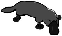
A duck-billed platypus. This platypus image was created by Jan Gillbank, English for the Australian Curriculum website (www.e4ac.edu.au). Used under Creative Commons Attribution 3.0 license.
Creating models that can identify queries as being sufficiently different from what was in a training dataset so as to be considered a new type of entity is a difficult research problem. Some of the areas of research relevant to this problem include outlier detection and one-class classification.
5.8 Exercises
1. The table below lists a dataset that was used to create a nearest neighbour model that predicts whether it will be a good day to go surfing.
ID |
WAVE SIZE (FT) |
WAVE PERIOD (SECS) |
WIND SPEED (MPH) |
GOOD SURF |
1 |
6 |
15 |
5 |
yes |
2 |
1 |
6 |
9 |
no |
3 |
7 |
10 |
4 |
yes |
4 |
7 |
12 |
3 |
yes |
5 |
2 |
2 |
10 |
no |
6 |
10 |
2 |
20 |
no |
Assuming that the model uses Euclidean distance to find the nearest neighbour, what prediction will the model return for each of the following query instances.
| ID | WAVE SIZE (FT) | WAVE PERIOD (SECS) | WIND SPEED (MPH) | GOOD SURF |
| Q1 | 8 |
15 |
2 |
? |
| Q2 | 8 |
2 |
18 |
? |
| Q3 | 6 |
11 |
4 |
? |
2. Email spam filtering models often use a bag-of-words representation for emails. In a bag-of-words representation, the descriptive features that describe a document (in our case, an email) each represent how many times a particular word occurs in the document. One descriptive feature is included for each word in a predefined dictionary. The dictionary is typically defined as the complete set of words that occur in the training dataset. The table below lists the bag-of-words representation for the following five emails and a target feature, SPAM, whether they are spam emails or genuine emails:
- “money, money, money”
- “free money for free gambling fun”
- “gambling for fun”
- “machine learning for fun, fun, fun”
- “free machine learning”

a. What target level would a nearest neighbor model using Euclidean distance return for the following email: “machine learning for free”?
b. What target level would a k-NN model with k = 3 and using Euclidean distance return for the same query?
c. What target level would a weighted k-NN model with k = 5 and using a weighting scheme of the reciprocal of the squared Euclidean distance between the neighbor and the query, return for the query?
d. What target level would a k-NN model with k = 3 and using Manhattan distance return for the same query?
e. There are a lot of zero entries in the spam bag-of-words dataset. This is indicative of sparse data and is typical for text analytics. Cosine similarity is often a good choice when dealing with sparse non-binary data. What target level would a 3-NN model using cosine similarity return for the query?
3. The predictive task in this question is to predict the level of corruption in a country based on a range of macro-economic and social features. The table below lists some countries described by the following descriptive features:
- LIFE EXP., the mean life expectancy at birth
- TOP-10 INCOME, the percentage of the annual income of the country that goes to the top 10% of earners
- INFANT MORT., the number of infant deaths per 1,000 births
- MIL. SPEND, the percentage of GDP spent on the military
- SCHOOL YEARS, the mean number years spent in school by adult females
The target feature is the Corruption Perception Index (CPI). The CPI measures the perceived levels of corruption in the public sector of countries and ranges from 0 (highly corrupt) to 100 (very clean).34

We will use Russia as our query country for this question. The table below lists the descriptive features for Russia.

a. What value would a 3-nearest neighbor prediction model using Euclidean distance return for the CPI of Russia?
b. What value would a weighted k-NN prediction model return for the CPI of Russia? Use k = 16 (i.e., the full dataset) and a weighting scheme of the reciprocal of the squared Euclidean distance between the neighbor and the query.
c. The descriptive features in this dataset are of different types. For example, some are percentages, others are measured in years, and others are measured in counts per 1,000. We should always consider normalizing our data, but it is particularly important to do this when the descriptive features are measured in different units. What value would a 3-nearest neighbor prediction model using Euclidean distance return for the CPI of Russia when the descriptive features have been normalized using range normalization?
d. What value would a weighted k-NN prediction model—with k = 16 (i.e., the full dataset) and using a weighting scheme of the reciprocal of the squared Euclidean distance between the neighbor and the query—return for the CPI of Russia when it is applied to the range-normalized data?
e. The actual 2011 CPI for Russia was 2.4488. Which of the predictions made was the most accurate? Why do you think this was?
 4. You have been given the job of building a recommender system for a large online shop that has a stock of over 100,000 items. In this domain the behavior of customers is captured in terms of what items they have bought or not bought. For example, the following table lists the behavior of two customers in this domain for a subset of the items that at least one of the customers has bought.
| ID | ITEM 107 |
ITEM 498 |
ITEM 7256 |
ITEM 28063 |
ITEM 75328 |
| 1 | true |
true |
true |
false |
false |
| 2 | true |
false |
false |
true |
true |
a. The company has decided to use a similarity-based model to implement the recommender system. Which of the following three similarity indexes do you think the system should be based on?
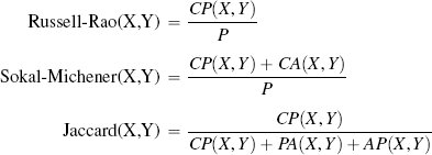
b. What items will the system recommend to the following customer? Assume that the recommender system uses the similarity index you chose in the first part of this question and is trained on the sample dataset listed above. Also assume that the system generates recommendations for query customers by finding the customer most similar to them in the dataset and then recommending the items that this similar customer has bought but that the query customer has not bought.
| ID | ITEM 107 |
ITEM 498 |
ITEM 7256 |
ITEM 28063 |
ITEM 75328 |
| Query | true | false | true | false | false |
 5. You are working as an assistant biologist to Charles Darwin on the Beagle voyage. You are at the Galápagos Islands, and you have just discovered a new animal that has not yet been classified. Mr. Darwin has asked you to classify the animal using a nearest neighbor approach, and he has supplied you the following dataset of already classified animals.
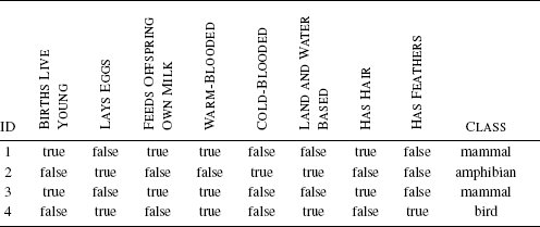
The descriptive features of the mysterious newly discovered animal are as follows:

a. A good measure of distance between two instances with categorical features is the overlap metric (also known as the hamming distance), which simply counts the number of descriptive features that have different values. Using this measure of distance, compute the distances between the mystery animal and each of the animals in the animal dataset.
b. If you used a 1-NN model, what class would be assigned to the mystery animal?
c. If you used a 4-NN model, what class would be assigned to the mystery animal? Would this be a good value for k for this dataset?
 6. You have been asked by a San Francisco property investment company to create a predictive model that will generate house price estimates for properties they are considering purchasing as rental properties. The table below lists a sample of properties that have recently been sold for rental in the city. The descriptive features in this dataset are SIZE (the property size in square feet) and RENT (the estimated monthly rental value of the property in dollars). The target feature, PRICE, lists the prices that these properties were sold for in dollars.
| ID | SIZE |
RENT |
PRICE |
| 1 | 2,700 |
9,235 |
2,000,000 |
| 2 | 1,315 |
1,800 |
820,000 |
| 3 | 1,050 |
1,250 |
800,000 |
| 4 | 2,200 |
7,000 |
1,750,000 |
| 5 | 1,800 |
3,800 |
1,450,500 |
| 6 | 1,900 |
4,000 |
1,500,500 |
| 7 | 960 |
800 |
720,000 |
a. Create a k-d tree for this dataset. Assume the following order over the features: RENT then SIZE.
b. Using the k-d tree that you created in the first part of this question, find the nearest neighbor to the following query: SIZE = 1,000, RENT = 2,200.
_______________
1 This example dataset is inspired by the use of analytics in professional and college sports, often referred to as sabremetrics. Two accessible introductions to this field are Lewis (2004) and Keri (2007).
2 The Manhattan distance, or taxi-cab distance, is so called because it is the distance that a taxi driver would have to cover if going from one point to another on a road system that is laid out in blocks, like the Manhattan road system.
3 In the extreme case with p = ∞ the Minkowski metric simple returns the maximum difference between any of the features. This is known as the Chebyshev distance but is also sometimes called the chessboard distance because it is the number of moves a king must make in chess to go from one square on the board to any other square.
4 A Voronoi tessellation is a way of decomposing a space into regions where each region belongs to an instance and contains all the points in the space whose distance to that instance is less than the distance to any other instance.
5 Instances should only be added to the training dataset if we have determined after making the prediction that the prediction was, in fact, correct. In this example, we assume that at the draft, the query player was drafted.
6 When using the reciprocal of the squared distance as a weighting function, we need to be careful to avoid division by zero in the case where the query is exactly the same as its nearest neighbor. Typically this problem case is handled by assigning the query the target level of the training instance d that it exactly matches.
7 See Section 3.1[56].
8 The primary papers introducing k-d trees are Bentley (1975) and Friedman et al. (1977). Also, note that the k here has no relationship with the k used in k nearest neighbor. It simply specifies the number of levels in the depth of the tree, which is arbitrary and typically determined by the algorithm that constructs the tree.
9 A binary tree is simply a tree where every node in the tree has at most two branches.
10 We use the median value as the splitting threshold because it is less susceptible to the influence of outliers than the mean, and this helps keep the tree as balanced as possible—having a balanced tree helps with the efficiency in retrieval. If more than one instance in a dataset has the median value for a feature we are splitting on, then we select one of these instances to represent the median and place the other instances with the median value in the set containing the instances whose values are greater than the median.
11 A hyperplane is a geometric concept that generalizes the idea of a plane into different dimensions. For example, a hyperplane in 2D space is a line and in a 3D space is a plane.
12 Similar to a hyperplane, a hypersphere is a generalization of the geometric concept of a sphere across multiple dimensions. So, in a 2D space the term hypersphere denotes a circle, in 3D it denotes a sphere, and so on.
13 Recall that each non-leaf node in the tree indexes an instance in the dataset and also defines a hyperplane that partitions the feature space. For example, the horizontal and vertical lines in Figure 5.9(b)[199] plot the hyperplanes defined by the non-leaf nodes of the k-d tree in Figure 5.9(a)[199].
14 Figure 5.12(a)[205] further misleads us because when we draw scatter plots, we scale the values to make the plot fit in a square-shaped image. If we were to plot the axis for the SALARY feature to the same scale as the AGE feature in Figure 5.12(a)[205], it would stretch over almost 400 pages.
15 For convenience we repeat Equation (3.7)[93] for range normalization here:

16 The example given here is based on artificial data generated for the purposes of this book. Predicting the prices of assets such as whiskey or wine using machine learning is, however, done in reality. For example, Ashenfelter (2008) deals with predicting wine prices and was covered in Ayres (2008).
17 These will be covered in Section 8.4.1[405].
18 One note of caution. The Jaccard similarity index is undefined for pairs of instances where all the features manifest co-absence as this leads to a division by zero.
19 The length of a vector, |a|, is computed as the square root of the sum of the elements of the vector squared:  .
.
20 If either vector used to calculate a cosine similarity contains negative feature values, then the cosine similarity will actually be in the range [− 1, 1]. As before, 1 indicates high similarity, and 0 indicates dissimilarity, but it can be difficult to interpret negative similarity scores. Negative similarity values can be avoided, however, if we use range normalization (see Section 3.6.1[92]) to ensure that descriptive feature values always remain positive.
21 Covariance between features means that knowing the value of one feature tells us something about the value of the other feature. See Section 3.5.2[86] for more information.
22 We explain covariance matrices in Section 3.5.2[86]. The inverse covariance matrix is the matrix such that when the covariance matrix is multiplied by its inverse, the result is the identity matrix: Σ × Σ−1 =  . The identity matrix is a square matrix in which all the elements of the main diagonal are 1, and all other elements are 0. Multiplying any matrix by the identity matrix leaves the original matrix unchanged—this is the equivalent of multiplying by 1 for real numbers. So the effect of multiplying feature values be an inverse covariance matrix is to rescale the variances of all features to 1 and to set the covariance between all feature pairs to 0. Calculating the inverse of a matrix involves solving systems of linear equations and requires the use of techniques from linear algebra such as Gauss-Jordan elimination or LU decomposition. We do not cover these techniques here, but they are covered in most standard linear algebra textbooks such as Anton and Rorres (2010).
23 The inverse of the identity matrix  is
is  . So, if there is no covariance between the features, both the covariance and the inverse covariance matrix will be equal to
  .
.
24 Section 3.5.2[86] describes the calculation of covariance matrices. The inverse covariance matrix was calculated using the solve function from the R programming language.
25 Recall that a dataset where the majority of descriptive features have zero as the value is known as sparse data. This often occurs in document classification problems, when a bag-of-words representation is used to represent documents as the frequency of occurrence of each word in a dictionary (the eponymous bag-of-words). The bag-of-words representation is covered more in Question 2[240] at the end of this chapter. One problem with sparse data is that with so few non-zero values, the variation between two instances may be dominated by noise.
26 A hypercube is a generalization of the geometric concept of a cube across multiple dimensions. So in a two-dimensional space, the term hypercube denotes a square, in three-dimensional space, it denotes a cube, and so on. A unit hypercube is a hypercube in which the length of every side is 1 unit.
27 This should not be confused with the concept of sparse data that was introduced earlier.
28 The discussion relating to the features of real data that help with the induction of models in high-dimensional spaces is based on Bishop (2006), pages 33–38.
29 Feature selection is sometimes also known as variable selection.
30 See Section 4.2.3[128].
31 We discuss the design of evaluation experiments in details in Chapter 8[397].
32 Obviously we must verify that the prediction made was correct before adding a new instance to the dataset.
33 The story recounted here of the discovery of the platypus is loosely based on real events. See Eco (1999) for a more faithful account of what happened and for a discussion of the implications of this discovery for classification systems in general. The platypus is not the only animal from Australia whose discovery by Europeans has relevance to predictive machine learning. See Taleb (2008) regarding the discovery of black swans and its relevance to predictive models.
34 The data listed in this table is real and is for 2010/11 (or the most recent year prior to 2010/11 when the data was available). The data for the descriptive features in this table was amalgamated from a number of surveys retrieved from Gapminder (www.gapminder.org). The Corruption Perception Index is generated annually by Transparency International (www.transparency.org).
