In this chapter, we will look at how to train and utilize machine learning models using BigQuery directly.
BigQuery ML (BQML) became generally available on Google Cloud Platform in May of 2019. The aim is to open machine learning models to a wider audience of users. Accordingly, BQML allows you to specify and run machine learning models directly in SQL. In most cases, you don’t need extensive understanding of the code required to produce these models, but a background in the concepts will still be helpful. Machine learning uses fairly accessible mathematical concepts, but as they are abstracted over many variables and iterations, the details get more difficult.
The next chapter will introduce Jupyter Notebooks, which will give a sense of how data science is typically done. The notebook concept now interoperates with Google’s AI Platform and BigQuery, so you can switch among the tools you’re most comfortable with. Before going into Python data analysis, we’ll go over the basic concepts using SQL in this chapter.
The crossover between data science and traditional business intelligence is the future of the field. Machine learning concepts have begun to pervade every industry. The power they’ve already demonstrated is astonishing. Within a few short years, classification and object detection algorithms have evolved to a high rate of success. Machine learning succeeds in places where humans might be unable to conceptualize a solution to a problem. Given some data analysis and some educated guessing, the model learns how to solve the problem on its own.
In June 2018, the GPT-2 text prediction model was released by the DeepMind AI Research Lab. This model is a general-purpose text generator capable of producing writing in nearly any format. Given a prompt, it will produce a plausible continuation of the text. This model can also take inspiration from the writer and will try to convey that writer's style. In fact, the italicized sentence was written by GPT-2. If you don’t believe me, try it for yourself and see.1
In April of 2020, OpenAI trained a neural net to generate raw audio containing music and even singing, based on training models consisting of numerical representations of music datasets and the text of the lyrics.2 In some cases it produces entirely new songs. While this is similarly impressive right now, we’re still only seeing the first fruits of machine learning.
This chapter has two goals: First is to introduce the basic concepts of machine learning to make BQML feel a little less magical. The second goal is to show you ways you can solve business problems with BQML. Both will increase your preparation for an increasingly ML-driven world and the new skill sets that data jobs require.
Fair warning: This chapter does vary both in tone and difficulty from the rest of the book. While BQML is easy to use, the underlying machine learning concepts are complex and are grounded in subject matter which is disparate from the rest of this book.
If this topic is of interest to you, there are several Apress books that explore this topic in significantly more detail.
Background
Machine learning and artificial intelligence are heavily burdened terms crossing multiple disciplines within mathematics and computer science. Before even delving into how to apply machine learning, let’s wade into the morass of ambiguous and confusing terminology.
Artificial Intelligence
Marketers often use the term “artificial intelligence,” or AI, and in recent years have begun to use the terms AI and machine learning (ML) interchangeably. As you may have heard, AI and ML are not the same thing.
History
Artificial intelligence has been a trope of human thought since antiquity. Over the centuries, AI appeared as a by-product of mythology, alchemy, or mechanical engineering. The intersection between artificial intelligence and prototypical computer science comes quite early. The story of the “Mechanical Turk” (the namesake of the Amazon product) tells of an 18th-century machine that could play chess. It enjoyed great success on multiple world tours, playing Benjamin Franklin, Napoleon, and other contemporary luminaries.3 Of course, the Mechanical Turk was in reality a person hidden underneath the table moving the pieces via magnets. However, in 1819, the Turk was encountered by Charles Babbage, the person who would later go on to invent the first mechanical computer. Babbage guessed that the Mechanical Turk was probably not an automaton. Nevertheless, it seems likely that the Turk was in his mind as he produced his first Analytical Engine in the 1830s. While Babbage invented the machine itself, the first person to truly see its potential as a thinking machine was his partner Ada Lovelace. Lovelace is the namesake of the programming language Ada and defensibly the first computer programmer.
The term “artificial intelligence” itself didn’t come into existence until 1955, when computer scientist John McCarthy coined the term.4 Since then, the term has proliferated into modern pop culture, inspiring authors like Isaac Asimov and in turn sentient synthetic lifelike Star Trek’s Mr. Data. The term is in general currency now to the point that it describes, essentially, computers performing any task that was typically done by humans. As a relative definition, it also means that it shifts as technology changes. In 1996, Deep Blue, the IBM chess-playing computer, famously defeated the world-reigning champion, Garry Kasparov, for the first time. At the time, this was the vanguard of AI. Some accounts of the time even claim that Deep Blue passed the Turing Test.5 As our capabilities grow and various entities persist in the claim that their simulations have passed the Turing Test,6 this definition has continued to grow and expand. In short, the term is weighted and conveys a great many things.
Machine Learning
Machine learning (ML) appears in the title of an IBM research paper by scientist Arthur Samuel in 1959,7 where he suggested that “Programming computers to learn from experience should eventually eliminate the need for much…programming effort.”8 This seems like a natural approach to artificial intelligence as an extension of the idea that humans gain intelligence through learning.
Essentially, ML is an approach to solving problems in the AI field. A coarse way to state this is to say that it uses data as an input to learn. This is obviously an oversimplification, as other AI techniques have inputs too. However, machine learning techniques build their models over the input of real observational data. Intriguingly, this also gives them a purpose that is somewhat distinct from classical AI. Typically, the standard for AI is to do things “like humans,” maybe faster or better, but still in a recognizably human way. Science fiction stories turn to horror when rogue AIs decide to take over. Whatever means they choose to do this, they still exhibit recognizably human motivations and ambitions.
Machine learning, on the other hand, is “interested” only in using data to create a model that effectively predicts or classifies things. The method by which it does this is not inherently important. Data scientists prioritize the characteristic of “interpretability,” meaning the model can be dissected and understood by humans, but this sometimes requires explicitly incentivizing a model to do so.
Interpretability
In a well-known example from 2017, Facebook researchers trained chatbots to barter basic objects such as books and hats with each other.9 In the initial model, the chatbots negotiated only with themselves and not other humans. After some time, they began to communicate using exchanges that appeared completely nonsensical to humans, such as “I can can I I everything else” and “Balls have zero to me to me to me to me…” This resulted in a lot of breathless media coverage about how the robots were evolving their own language. They would accordingly take over the world, bent on enslaving humanity to make their books, balls, and hats for all eternity.
In reality, this model was simply not easily “interpretable” by humans. The algorithm drifted away simply because there was no incentive for the chatbots to use English. The researchers tweaked the algorithm to reward humanlike speech, creating a more interpretable and slightly less effective model.
In its quest for optimization, machine learning will take any path that improves its results. There are several entertaining examples where machine learning models (and other artificial intelligence) exploit the simulations themselves to produce unintended but “correct” results.10 One common theme is that the model will learn to delete its inputs altogether and produce an empty output set. In doing so, these models score perfectly over the zero evaluated outputs. For example, a model optimized to sort lists simply emitted empty lists, which are technically sorted. In another similar example, the candidate program deleted all of the target files, ensuring a perfect score on the zero files it had processed.11 (There is an odd parallel to the AI from the 1983 movie WarGames, who discovers that “the only winning move is not to play.” Riffing off of this, the researcher Tom Murphy, teaching an algorithm to play Tetris, found that the algorithm would pause the game forever to avoid losing.12)
Statistics
Machine learning isn’t just statistics, either. Understanding statistical methods is important to building good machine models, but the aims of each are not fully congruent. The relationship between statistics and ML is somewhat like the relationship between computer science and software engineering. The theoretical/applied gap comes into play in a big way.
Statistics is mathematically rigorous and can be used to express some confidence about how a certain system behaves. It’s used academically as a building block to produce accurate conclusions about the reason that data looks the way it does. Machine learning, on the other hand, is most concerned with iterating to a model that takes input and produces the correct output. Additional input is used to refine the algorithm. The focus is much less on the “why” and more on how to get the algorithm to produce useful results.
Of course, ML practitioners use statistics and statisticians use ML methods. There’s too much overlap for this to be a useful comparison, but it comes up a lot and is worth touching upon. To the math/CS analogy, imagine wanting to know the circumference of a circle. Inevitably, the value of π arises in the process. In the algorithmic view, it’s a means to an end—we want to derive a sufficiently accurate value to calculate the circumference of any circles we may encounter. We could do this with measurement or a Monte Carlo method and create a ratio between circumference and diameter that we’d be quite happy with. However, from the mathematical perspective, we want to prove the value of π itself to show “why” it arises in so many contexts and how it is related to other mathematical concepts.
There’s an interpretability factor here, as well. ML models, unless incentivized to do so, can produce pretty opaque results. It may not be trivial or even possible to understand why a model produces extremely accurate predictions or descriptions of certain phenomena. We may apply a statistical method to a machine learning model in retrospect and discover that it’s extremely accurate and still not know why. Statistics, on the other hand, has the ability to formulate intelligent conclusions that help us understand the phenomena under study and their possible origins or relations to other disciplines. And that’s about as granular as is sensical.
Ethics
A discussion of machine learning requires some review of the ethical implications. As custodians of data, we may have access to privileged information including financial or health information, private correspondence, or even classified data. In the aggregate, we may not think much about the value of each data point. However, machine learning models have the potential to affect millions of lives both positively and negatively. Before we jump into BQML, here’s a quick refresher.
Implicit Bias
Implicit bias refers to unconscious feelings or attitudes that influence people’s behaviors or decisions. These attitudes are often formed starting an early age by messages from surroundings or from the media.
When it comes to machine learning, these biases can find their way into the training models in nonobvious ways. One example is if certain language carries coded meaning that is more often used to describe people of particular classes. An ML model might pick up on these distinctions and amplify a bias where none was intended. This could adversely affect a scoring or prediction model, like an application for a loan or a hiring candidate.
Disparate Impact
When a machine learning model is implemented that contains these biases, it can create the possibility for disparate impact. This arises when a seemingly neutral decision-making process unfairly impacts a certain group of people. This could happen very easily—say that certain data points are more commonly missing for certain classes of people, either due to data collection methods or cultural sensitivity. Dropping those data points could cause the affected people to be underrepresented in the data model.
Another scenario highlights a deficiency of statistical learning models. What if the built model in fact contains no implicit bias and correctly represents the state of the world? This may reveal ugly imbalances that do not represent the world as we hope or wish it to be. In that case, the machine learning model is doing exactly what it is “supposed” to do, but it does not get us where we are trying to go.
Responsibility
Many practicing professions require licensure—lawyers, doctors, architects, and civil engineers come to mind. Software and data engineering generally do not, with scant few exceptions. A code of ethics for software engineers was approved in 1999 by the IEEE-CS/ACM Joint Task Force and clearly lays out the professional obligations of software engineers.13 Terms like “big data” and “cloud computing” were still several years in the future, but computer scientists had a good idea of what lay ahead.
Careless or malicious code can cause catastrophic loss of monetary value or human life.14 The twist with machine learning, as applies to both interpretability and power, is that it can take actions humans might consider unethical, even when programmed by humans with the best intentions. It’s too easy to say “the algorithm did it” when something goes awry. This may sound preachy, but the ease of integration brings this power so close to hand. When it’s all there at your command, it’s easy to forget to think about your responsibility in the equation. To the preceding question of disparate impact, the code of ethics states it directly: “Moderate the interests of the software engineer, the employer, the client and the users with the public good.”15
BigQuery ML Concepts
BigQuery ML follows a theme familiar to other services we’ve discussed—it takes a concept from another domain and implements it using familiar SQL. This makes it accessible to data analysts who may not have substantial experience with machine learning. It also provides a gentle slope into more complex topics by allowing the direct implementation of TensorFlow models. As your skill naturally grows through application, you can take on more advanced implementations. In the following chapter, our examples will be in Python as we survey the data science landscape outside of BigQuery.
BQML implements a natural extension to SQL to allow for prediction and classification without leaving the BigQuery console. However, you probably will want to, in order to visualize your results or to work with the model training directly. In general, BQML is great for creating inline models that you can use without a deep understanding of either statistics or machine learning. Options like AutoML and TensorFlow (which we’ll look at in the next chapter) become more appropriate as your investment in ML techniques grows.
Cost
If you are on a flat-rate plan (see Chapter 4), your BQML costs are included with your plan, so you can skip over this. Matrix factorization, in beta as of this writing, is only available through a flat-rate plan or flex slots.
The cost calculations follow the same rules as regular BigQuery for storage and querying, including ML analysis. The free tier includes the same amount of storage and data processing, and any ML queries you run on existing models will be factored into that price.
Machine learning of any type can get expensive pretty quickly. This shouldn’t be a deterrent—the free tier is more than enough for learning the ropes and doing some decent-scale models. (At least in BQML. AutoML Tables, which we’ll cover in the next chapter, has a free trial but no free tier.) As with cost analysis for BigQuery as a whole, assess your intended scale and usage and decide what makes sense. At anything approaching the upper end, you’ll be working with Google instead of paying list price, anyway—tell them I told you to give them a discount. (Your results may vary.)
Creating Models
With model creation, there are some additional costs. BQML model creation (i.e., any job including a “CREATE MODEL” statement) is billed at a different rate and has a different free allotment. The free tier is currently 10 GB of processing data during model creation, after which the price (as of this writing) goes to $250/TB for US multi-region. Recall that multi-region is cheaper than single region because the query can be redistributed according to need.
This creates two separate problems for cost tracking. First, since ML analysis and queries are bundled into the regular analysis pricing, there’s no simple way to separate your ML analysis costs. It might seem like there is no reason to do this, but when a cost-conscious executive suggests that artificial intellige-ma-what is costing the company an arm and a leg, it could be useful to be able to separate those costs. (Of course, on a flat-rate plan it’s all “data warehouse” anyway.)
The second issue is that model creation costs are not itemized at all—on your monthly statement, they’re going to get bundled in with the rest of the BigQuery costs, even though model creation is billed at a different rate. There is some documentation that implies that this limitation will change at some point, and perhaps queries that invoke ML functionality will also get a separate line item.
If you are really interested in how to show individual model creation costs, you’ll have to go into Cloud Logging (see Chapter 12). The BQML documentation has a tutorial16 on how to do this. No doubt, there is a fun infinite loop (and infinite bill) for those who want to use BQML to predict how much they will spend on BQML over time.17
Flex Slots
Flex slots are a new pricing concept that is essentially a time-bounded flat-rate pricing. The minimum reservation is only 60 seconds, and slots are charged per second. This pricing model is considerably more expensive over the long term than actual flat rate—46% at list price for US multi-region. However, for short-term or bounded needs, it can be used without requiring a full flat-rate commitment or reservations.
Any models that use matrix factorization are only available via flat rate, reservations, or flex slots. While flex slots are still basically a “pay-as-you-go” model, it’s worth planning ahead of time how much you intend to use these models and what the right approach is.
Since it’s only the CREATE MODEL calls that are billed separately, it might be possible to create a factorization model using flex slots and then utilize its predictions with regular BigQuery. I did not personally attempt this, but it seems like a possibility.
Supervised vs. Unsupervised Learning
BQML supports two major classes of learning models, supervised and unsupervised. The major difference between the two types is simply whether the model has access to “ground truth”—essentially, objective reality measured empirically. You can use a combination of both or even use unsupervised model results as ground truth for supervised models.
Supervised Models
In a supervised model, you supply some data which is already labeled, that is, it contains both the input and your expected output. Regression is a good example of a supervised model; in order to predict numerical values, the model needs to know existing data relationships. For example, to predict home prices, a regression model needs to know the historical prices of houses sold, as well as other salient features of the data. This is the “ground truth” for a supervised model. By testing your supervised model on facts you know, but your model has not yet seen, you can test its accuracy.
Less than 500 rows: 100% of data goes to validation.
Between 500 and 50,000 rows: 80% of data goes to training and 20% to validation.
Over 50,000 rows: More than 80% of data goes to training; 10,000 rows go to validation.
You can set this directly if you want, either with a percentage or with a BOOL column to say whether the row is for training or evaluation.
Supervised models typically have an additional split in the test data between validation (biased testing while tuning) and testing (unbiased data the model doesn’t see until the end). AutoML Tables, which we’ll talk about in the next chapter, lets you add a column to specify directly which of the three you want each row to do. AutoML Tables also uses a default of 80/10/10 (training/validation/testing).
Unsupervised Models
Unsupervised models , by contrast, don’t have any labeled data. Generally this is because there is no specifically desired outcome. Unsupervised models will search for and extract relationships in the data and then produce clusters or detect anomalies in the data. BQML natively supports k-means clustering, which is covered in more detail in the following, followed by an example.
Unsupervised model results are often useful as a subsequent input to supervised models. They can be used to create groups of similar data points, and then that grouping can be used as an additional feature in a supervised model to increase its predictive capability. Of course, it can amplify biases in the unsupervised results too.
On their own, unsupervised models are well suited to identifying patterns unseen to human observers. Fraud detection, data loss prevention, or unusual system behaviors can all be detected by unsupervised models.
Model Types
BQML supports the most common types of both supervised and unsupervised models. There are other types of models and plenty of other variants on the ones given in the following.
This section contains a lot of math and statistics to illustrate how the various models and metrics work. Don’t let that scare you off—they’re not necessary for comprehension, and in fact you can use BigQuery ML without much of this information at all. However, your ML intuition will be much stronger if you understand how to assess the performance of your model. This is especially good if you have limited resources and want to stop when you believe the results are “good enough.”
Linear Regression Models
Linear regression models are supervised models which generate a function to predict output based on input. Generally, the input features will predict a target value using the function that the model computed.
It works just like a statistical linear regression. Known data points are plotted (“ground truth”), and then a line of best fit is found. Since this technique is mathematical, the labeled inputs must all be real numbers. You can address yes/no variables by assigning them numerical values like {1.0, 0.0}, and you can address variables with a fixed number of choices as {0.0, 1.0, 2.0, ...}. BQML will do this for you automatically.
Linear regressions can be done over multiple variables. In statistics, you take real information about your data and use it to choose appropriate variables. The goal of the statistical analysis is to come up with intelligent theories about which variables are responsible for changing the outcome. In machine learning, you throw every possible combination at it, potentially thousands or millions of terms. You run them all and see how it goes. If the model predicts better with half the variables removed, you take them out and try again. This would be considered a pretty severe lack of rigor as a statistical practice. In machine learning, it’s looking over the largest possible problem space to get the most predictive function. This isn’t brute force, exactly, but it definitely takes advantage of modern parallelization and computation to examine as many results as it can .
RMSE
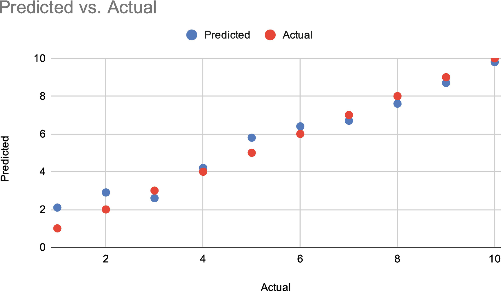
Line of best fit with RMSE

- For each point in the set
Subtract the observed value from the predicted value.
Square it.
Find the average of all of these squares.
Take the square root of that average.
RMSE is an example of a “loss function,” since for a set it tells you exactly how much fidelity is sacrificed by using this linear regression model. Improving linear regression models means optimizing the loss function, and thus a lower RMSE means a better model.
This will come up in the next chapter as well, but if your RMSE is zero, that is probably not a good thing. A perfect fit means your test data and your predictions are an exact match. This is referred to as “overfitting”—the model corresponds so well with its training data that either there is an obvious relationship somewhere or it will be brittle when it encounters new data.
Overfitting
If there is an obvious relationship somewhere, this is often referred to as “data leakage.” Data leakage is a problem with a supervised model where some features accidentally expose information about the target value. This leads the model to pick up a relationship that won’t be present in real-world data. The model will likely be useless in the real world, because the features it determined to calculate the best fit won’t be present or will not follow the pattern.
A great example of this is when the row number of the data makes it into the model. For example, say you want to predict how many people in a given zip code will purchase a specific product this year. One good training input might be the purchases by zip code from last year, so you prep the data. However, it is accidentally sorted by increasing number of purchases and also contains the original row number from the source table. So row 1 is someone who purchased $0 last year, and the last row is the biggest spender. The regression analysis is going to detect that there is a strong correlation between “row number” and total spending. Essentially this is like saying, “Oh, those row number 1s. They never buy anything!” Your real-world datasets aren’t going to come with row number labels—that information only exists retrospectively as the data was collected. But that model would probably score an RMSE of pretty close to zero, and not for the reasons you want.18
Classification Models
The other major type of supervised model is the classification model. In a classification model, the goal is to classify data so that the result predicts a binary or categorical outcome.
The canonical example is spam filtering. In a spam filter algorithm, the features would be things like email body, subject line, from address, headers, time of day, and so on. The output from the binary classifier would be “spam” or “not spam.” Similarly, you could predict a category based on the input. For example, computer vision often uses images or videos of real objects (supervision) and then can train itself to categorize pictures of other objects. If you train a supervised classification algorithm on five different kinds of trees, the output will be able to receive a picture as input and respond with a classification (i.e., oak, birch, pine, jungle, acacia).
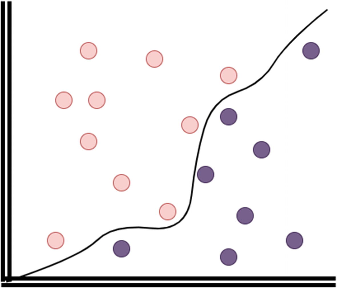
Classification model
At its most basic, a classification model is a linear regression model with discrete outputs. There’s an underlying prediction value (i.e., this email is 0.4 SPAM so therefore it is not spam). Confidence values can be obtained in that way.
You can also test the model in a similar way, by simply assessing what percentage of classifications were made correctly on the test data. This has a drawback, which is that it doesn’t take into account the data distribution. If data is strongly imbalanced between “yes” and “no,” then the model could be right solely by predicting that answer every time. For example, if 99% of customers are repeat purchasers, and the model says “yes” to every input, it will be 99% correct, which looks good, but reflects the data more than the model. This metric is called “accuracy” in ML, and it’s necessary but not sufficient.
Precision and Recall
An additional way to show the performance of a classification model is to look at false positives and negatives as well as correct predictions (“accuracy”). (You may recognize these as Type I and Type II errors from statistics. In machine learning, these ideas are captured in two terms, known as precision and recall. Recall is sometimes known as sensitivity, but BQML is consistent in the use of recall.)
Judging by the amount of blog entries and web pages purporting to explain the definitions of these terms, they must be challenging to understand.
Precision and recall are both measured on a scale of 0.0–1.0. A perfect precision of 1.0 means that there were no false positives. A perfect recall of 1.0 means there were no false negatives. Stated in reverse, precision measures how accurate your positive identifications were. Recall measures how many of the positive truths you identified (labeled as positive).
The extreme cases are useful here in describing the boundaries. Let’s take the preceding spam example. Say you have ten emails and they’re all legitimate. By definition, precision is going to be 1.0 as long as a single positive identification is made—no matter which emails you say are legitimate, you’re right. However, for every email you incorrectly class as spam, the recall score drops. At the end, if you say six of the ten emails are legitimate and four are spam, you have a precision of 1.0—six out of six identifications were right. Your recall is only 0.6 though, because you missed four emails (0.4) that were also legitimate.
Same example, but opposite case. Now you have ten emails, and they’re all spam. In this case, if you identify even a single email as legitimate, your precision will be 0.0, because every email you identified as legitimate was spam. Recall, on the other hand, will be 1.0 no matter what you do, because you found all of the zero positive results without doing anything. So if you make the same determination—six emails legitimate, four spam—those are the results you’d get: 0.0 precision, 1.0 recall.

Confusion matrix followed by calculations
This is sometimes referred to as a confusion matrix, which is intended to refer to the classification of the dataset and not its reader.
You may also have noticed one odd thing about the preceding cases, which is that following this formula, the recall calculation appears to produce division by zero. By convention, since we’re actually talking about sets here and not numbers, this question is really asking what ratio of items in the set were identified—the denominator set is empty (∅) so recall is 1.0.
This also illustrates why both precision and recall are necessary to see how accurately a model worked as a classifier. Generally, as you try to increase precision to avoid making an inaccurate result, recall goes down because you didn’t get all the results. If you go for broke and just return every item in the set, your recall will be perfect but your precision will be terrible.
When you evaluate a logistic model using BQML, it will automatically return the accuracy, precision, and recall of the model, as well as a few other metrics.
Logarithmic Loss
The most common method for evaluating a classification model is logarithmic loss . This is a loss function specifically for logistic regression that essentially measures the prediction error averaged over all samples in the dataset. It’s sometimes called “cross-entropy loss,” referring to the loss between the actual dataset and the predicted dataset. Minimizing cross-entropy maximizes classification.
In practice, log loss improves (decreases) for each correct prediction. It worsens (increases) for each wrong prediction, weighted by how confidently that incorrect prediction was made. The output for a logistic classifier will ultimately be either 0 or 1, but it still reflects an underlying probability, which is selected based on the threshold. The log loss calculates this discrepancy across all thresholds.
The value of the log loss function in measuring the performance of your model will vary based on whether it’s binary or multi-class. It will also vary if the probability of both 0 and 1 in the real dataset is even, like a coin toss, or if it is heavily imbalanced in one direction or another.
F1 Score
The F1 score, so named by apparent accident,20 gives equal weight to precision and recall by calculating their harmonic mean.
Harmonic means to show up in lots of places where the two components influence each other in a way that would bias the arithmetic mean. Basically, both precision and recall are related by the numerator and are already ratios themselves. The canonical example is average speed on a train trip; if you go 40 mph outbound and 120 mph inbound, your average speed was not 80 mph. The ratio of miles over hours means you spent less time at 120 mph to go the same distance. So, if the destination were 120 miles away, this means it took 3 hours at 40 mph one way and 1 hour at 120 mph on the return—the average is actually ((3*40)+(1*120))/4, or 60 mph.

Since precision and recall are both between 0.0 and 1.0, the F1 score is also bounded between 0.0 and 1.0. (Plug 1.0 into both precision and recall, and you’ll see it yields 1.0, the same as the arithmetic average. If both precision and recall have the same value, the harmonic mean will equal the arithmetic mean.)
This score is only useful if you believe that precision and recall have equal weight. An extended version, Fβ, allows you to bias either precision or recall more heavily and could be considered a weighted f-measure.
ROC Curves
An ROC curve, or receiver operating characteristic curve, is another common way to measure the quality of a binary classification model. Developed in World War II, it refers literally to the recall (sensitivity) of a radar receiver at distinguishing birds from enemy aircraft.21 It describes the tension covered in the “Precision and Recall” section. As the sensitivity of the receiver was turned up, it began to lower precision as more false positives were identified. Leaving the sensitivity low ran the risk that enemy aircraft would fly over undetected (false negatives). Using the ROC curve helped to find the optimal setting for recall that yielded the highest precision while maintaining lowest number of false alarms.
The ROC curve uses a measure called specificity, which is the proportion of true negatives correctly identified. Note that while precision and recall both focus on performance of correct positive identification, specificity looks at correct negative identification.
An ROC curve is a two-dimensional graph showing a line, where inverted specificity (1-specificity) is on the x-axis and recall (sensitivity) is on the y-axis. As the origin indicates, it plots hit rates (enemy aircraft) vs. false alarms (geese). Along the curve, you can see the average specificity for all values of recall from 0.0 to 1.0 (or the converse).
The reason the curve is so useful is because depending on the problem you are trying to solve, a greater degree of false positives may be acceptable, especially when the cost for a missed identification is high. For example, in any test to detect a disease, a false positive is usually better than a false negative.
When using BQML, the metric returned is called roc_auc, which refers to the calculation of the area under the curve of the ROC. The area of a 1-by-1 plot is also 1, which means that the maximum area under the curve is also 1.0. A perfect roc_auc score means that the diagnostic accuracy of the model is perfect—it gets both the positive and negative cases accurate in every case.
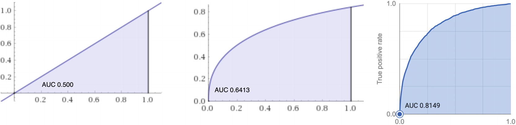
Several plots of roc_aucs graphed together
Where roc_auc can be extremely useful is in comparing the characteristics of two different models. Plotted along the same axes, you can make an apples-to-apples comparison of which model performs “better” without looking at the curves themselves.
To calculate the area under the curve, you can use the trapezoidal rule.22 Since the roc_auc is a definite integral, you don’t need calculus integration techniques to work it out. Or even better, just let BQML tell you the answer.
TensorFlow Models
TensorFlow fills hundreds of books on its own, so by necessity this is only a brief summary. We’ll also touch upon TensorFlow in the next chapter. Essentially, TensorFlow is a Python-based platform for machine learning models. TensorFlow is one of the two most popular Python ML platforms (along with PyTorch), enjoying a robust community and lots of documentation and support. Google supplies its own quick introduction to classification in TensorFlow, in concert with a higher-level library called Keras.23
For our BQML purposes, in late 2019, importing TensorFlow models into BigQuery reached general availability. This bridged existing machine learning practice directly into BigQuery, allowing data analysts to directly utilize and incorporate custom ML models into their work.
To load one in, you can create a model of type TENSORFLOW using a Google Cloud Storage location where the model has been stored. BQML will automatically convert most common data types back and forth. Once you’ve imported the model, it’s locked into BQML.
TensorFlow models in BQML support the common prediction methods, but you won’t have access to the training and statistics. For example, you can’t evaluate a TensorFlow model to see its performance nor examine its features. Models are also currently limited to 250 MB in size, which may not cover larger scale.
Nonetheless, this feature addresses a key concern around the initial BQML release, namely, that custom-tuned TensorFlow models were more accurate and suitable for production workloads. Now, as a data analyst, you could create a BQML model by yourself and begin using it. Once the data science team returns to you a TensorFlow model with more predictive capability, you could silently replace the native BQML model with the TensorFlow model and take advantage of it immediately.
K-Means Clustering
K-means clustering describes an unsupervised machine learning algorithm that performs segmentation on a dataset. The name comes from the algebraic variable k, indicating the number of clusters to produce, and mean as in the statistical average of each cluster. As it is unsupervised, k-means clustering can perform this segmentation without any input on the salient features.
In brief, the algorithm selects k random data points and assigns them as representatives for the clusters. Then, the other points are taken in and calculated for similarity to each of the representatives. Each row is grouped with its closest representative. Then, representatives are recalculated using the arithmetic mean of the current clusters, and the process is repeated. After enough iterations, each cluster’s arithmetic mean, or centroid, stabilizes and future iterations produce the same k arithmetic means. At that point the data has been successfully grouped into k segments, where each segment has a mean that averages all the data points in that segment.

K-means graph, unsorted
 . (Huh, this looks a lot like the RMSE calculation…) Each data point is also an (x,y) coordinate, and its distance to each of the k centroids is calculated accordingly. The point is assigned to the centroid which is closest. After this iteration, the two-dimensional mean of each cluster is calculated, and those values are assigned as the k centroids for the next iteration. Rinse and repeat. Eventually, the centroids converge and stop moving around (stabilize). The data is now segmented into k groups, with each group being compactly described by an average. See Figure 19-6.
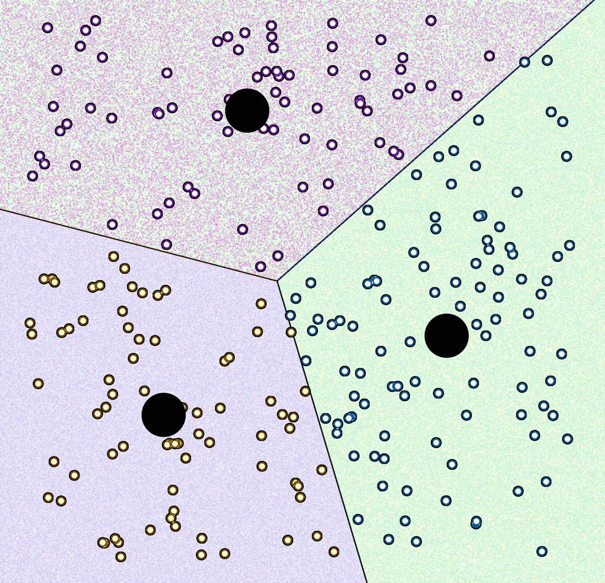
K-means graph, complete
When we look at this in BQML, the equivalent is a k-means model on a two-column table. We can certainly add more columns. The equation for Euclidean distance works in higher dimensions as well, by adding the terms ((z1 − z2)2 + (a1 − a2)2…) under the square root, but this gets pretty difficult to visualize above three.
Procedure
The process for implementing BQML is similar across all types of models. This section will review the general steps, before applying them to a few examples in the following sections.
Prepare the Data
In order to create the model, you first need to prepare your input dataset. Typically this will be a subset of raw data that you believe is salient to answering the business question at hand. This may also include some exploratory data analysis (which will be covered more deeply in the next chapter) and column selection. In some types of supervised learning, you may also need to annotate the data with information about how the model should treat it or to be able to look back at a model’s quality.
If you’re drawing data from multiple sources, you may also need to construct the subquery or table joins required to collect the input data into the same location. Note that you can use regular or even materialized views as the input source for BQML models, so you don’t need to explicitly copy the data in the preparation step.
In the next chapter, we’ll do some model generation without much explicit preparation at all. This preparation procedure should be used on any models for BQML, as well. The nice part is that the majority of these techniques are the same as you would do for regular data cleaning when loading data into a BigQuery warehouse.
Remember that for the purposes of BQML, when we talk about “features,” we’re talking about a table column that will go into the model.
Data Distribution
Depending on your dataset, you may not want outliers in your model. The rule of thumb for eliminating outliers is generally the same. If you have a normal data distribution, generally you want to eliminate values that fall outside of three standard deviations from the mean.
Again, because of the vast amount of rows and columns you may be analyzing, it’s worth looking at outliers to see if you can pinpoint a cause. For example, I was once trying to analyze a dataset of prices with two maxima, one at the far left and one at the far right. The mean was useless, and most data points qualified as outliers by the standard definition. When I went to look at the dataset, I realized that most of the rows were decimal, that is, 4.95, but a significant set were measured as pennies in integers, that is, 495. I multiplied all decimal values by 100 and the data suddenly made sense. (Yes, I did account for decimal values that fell within the range, i.e., $495.)
Sometimes data collection methods are bad or an error produces unhelpful data. If there are a lot of maxint or other sentinel-type values in the data, this could be an indication of that. In some extreme cases, the dataset may be unsuitable for processing until these errors have been corrected and the data reimported.
Missing Data
Real-world datasets are likely to have missing data. Deciding what to do about this is highly model-dependent. In general, removing columns or rows with mostly missing data is preferable. Consider disparate impact when you do this though: why is the data missing?
Normally, you might also consider imputing data. If the data is missing only in a small number of rows and the distribution is normal, you can “make up” the remainder of it by filling in the average. Luckily, BQML will do this for you, so you need only decide whether you want the row or column at all.
Label Cleanup
Depending on the method of data collection, columns may have spelling or labeling variations to represent the same items. If you’re using properly normalized data, you can use the IDs (but mind leakage). Otherwise, you may want to do some alignment to make sure that you use the same string identifier to mean the same class. For example, if your accessory type column has “Women’s Shoes,” “Shoes – Female,” “Women’s Shoes size 6,” and so on, you will want to regularize all of those to “Women’s Shoes” if that feature is important to you.
Feature Encoding
Feature encoding is another task that BQML will handle when you create a model. If there is some reason that it should be done outside of the BQML model creation—that is, you want to use the dataset with Python libraries or you want to combine encoding with data cleanup—you can do it yourself. Here are some of the techniques BQML performs on your input data, since they’re good to know.
Scaling
Scaling, or “standardization,” as Google refers to it, reduces integer and decimal values to a range centered at zero. This means all values will normalize into relative distances from zero, meaning that numeric features can be compared in a scale-agnostic fashion.
One-Hot Encoding
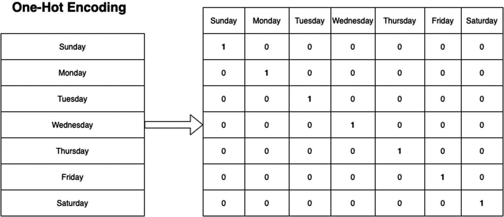
One-hot encoding with days of the week
The reason for this is that it allows each feature to stand on its own. For example, if you needed to convert the days of the week into one-hot encoding, you’d end up with seven columns, one for Monday, one for Tuesday, and so on, where only one of the values could be on (“hot”) at a time. This would allow for a single day of the week to shine through as an individual feature if it made a major impact on the predictions. While you might be inclined to think of these as seven separate booleans, all features are numerical, so it’s actually 0.0 or 1.0.
Another reason for this is that converting categorical data into numerical data might imply scale where none exists. If Monday were 1 and Saturday were 7, that could translate to Saturday being “more” than Monday. It would also lead to nonsensical decimal predictions; what day of the week is 4.1207?
On the flip side, if your categories are ordered or sequenced in some way, you can leave them in numerical form to reflect their relationship. For example, encoding gold, silver, and bronze as 1, 2, and 3 could make sense. While you’ll still get nonsensical decimal predictions, the meaning is slightly more intuitive.
Multi-hot Encoding
Multi-hot encoding is used specifically for transforming BigQuery ARRAY types. Like one-hot encoding, each unique element in the ARRAY will get its own column.
Timestamp Transformation
This is Google’s name for deciding if BQML will apply scaling or one-hot encoding to timestamp values based on the data type and range.
Feature Selection
Feature selection is the process of choosing which features (columns) make sense to go into the model. It’s critically important and BQML can’t do it for you, because it relies on understanding the problem.
First and foremost, the computational complexity (read: time and money) of the model goes up with the number of features included. You can see with one-hot encoding and large datasets how the number of features could easily go into the hundreds or thousands.
Second, you reduce interpretability when there are too many features in the model to easily understand. Often, the first order of approximation is good enough, which means while all those extra features are slightly increasing the performance of your model, it’s not worth the concomitant reduction in comprehension.
Lastly, the more features you use, the more risk there is of overfitting your model or introducing bias. It certainly raises the chances of accidentally adding the row number or something like it. With respect to bias, it could cause the model to reject all loan applications for people with a certain first name. While it very well may be that people named Alastair always default on their loans, it would be hard to assess that as anything more than coincidental.
There are many ways of doing feature selection. For BQML models, you might just go with your gut and see what happens. There are also some statistical methods you can use to assess the quality of various features on your model. For supervised models, you can use Pearson’s correlation to calculate how significant each feature is in predicting the target value.
BigQuery supports this as a statistical aggregate function called CORR, which was conveniently ignored in the chapter about aggregate functions (That was Chapter 9.) CORR will look at all the rows in the group and return a value between -1.0 and 1.0 to indicate the correlation between the dependent and the independent variables. (You can also use it as an analytic function if you need windowing.)
This is just the tip of the iceberg. Many other functions like chi-squared and analysis of variance (ANOVA) can also be used to help with feature selection. Neither of those is built into BigQuery, although you can certainly find plenty of examples in SQL. (Or use a JavaScript UDF!)
It is also possible (though not built into BQML) to use statistics to perform automatic selection to optimize to the metrics you select. However, doing this properly requires actually running the model and calculating the metrics, mutating it, and then doing it again. Looking at all possible combinations across hundreds of features is effectively impossible, and so automated feature selection relies on making good choices based on the available statistical information. There are a number of methods for doing this. In practice, using available Python ML toolkits is the best way, and in the next chapter we’ll look at integrating Python with BigQuery so you can move seamlessly between the two.
Feature Extraction
Whereas feature selection refers to choosing from the columns you already have, extraction refers to creating new columns using available data. Feature encoding and imputation could be seen as a form of extraction, but it generally describes more complex processes. The goal is to synthesize data points which better reflect the problem under consideration. Sometimes it’s a necessity. When you’ve performed feature selection and the remaining features are too large to fit into your available memory, you need to find a way to represent them more compactly without losing too much fidelity.
Feature extraction is especially important on datasets with a lot of extraneous data. Audio and video are too large to process uncompressed in their entirety. In fact, when the Shazam algorithm for music identification was invented25 in 2003, its revolutionary approach involved feature extraction. As a drastic oversimplification, audio tracks are reduced to discrete hashes based on peak intensity over time. When a recording for identification is made, it undergoes the same hash algorithm, and the database is searched for a match. The features that were extracted are invariant (for the most part) under background noise, and clustering techniques (like k-means) can be used to find likely matches.26
One basic feature extraction technique is setting a threshold you know to be good and using that to define a boolean. For instance, if you know that a credit score over 800 is “exceptional” and you feel that this problem is likely to care about that specifically, you can define a new feature which is just (credit score > 800) = 1.0.
BQML also provides a number of feature extraction methods, which they refer to as “preprocessing functions.” These include scalers, bucketizers, and combiners. You can use these in combination with ML.TRANSFORM when creating your model.
One common feature extraction method that isn’t easily described by the preceding techniques is known as “bag of words” in ML. The bag of words model converts text into a list of words and frequencies, either by total count or ratio. This gives ML models a predictable feature as opposed to a mess of text. Text preprocessing also includes filtering punctuation and removing filler words.
The bag of words model is a valuable preprocessing step for natural language analysis. It’s extremely useful for sentiment analysis, that is, deciding if a particular text is positive or negative. While general sentiment analysis can be performed without machine learning, you can use this technique as a classifier for sentiment analysis in your specific domain. For example, you could run it on all of the tickets and emails your call center receives, allowing the prediction of sentiment specifically on relevant data to you. While general sentiment analysis classifies something like “It's been a month since I asked for a replacement” as neutral, your domain-specific classifier could learn that the customer was unhappy. You can use this method on BigQuery with the ML.NGRAMS keyword.
ML.TRANSFORM
The TRANSFORM keyword is used to perform both feature selection and extraction while creating the model. Since it is possible to specify only certain columns, selection is built in, after the hard work of deciding which those are. Transformation is accomplished using preprocessing functions like scaling and bucketizing. Finally, BQML does encoding on its own with whatever data types it gets.
We’ll see this in action in the examples.
Create the Model
Next, you create a model using. SQL. This SQL statement handles the creation and training of the model using the input data that you have supplied. It also creates a BigQuery object to represent the model. In evaluation and prediction, the model name is used as the reference.
This means you can create multiple models of different types using the same input data and then perform predictions and compare them. This is known as “ensemble modeling.” When multiple models agree on a result, it adds weight to the prediction. Of course, as discussed earlier, this can also get quite expensive.
To do this, you run the CREATE MODEL statement and indicate which kind of model to create, as well as the features to be included.
Evaluate the Model
For all model types except TensorFlow, you can then use ML.EVALUATE to see the performance of your model. Depending on the type of model, the returned statistics will be different. For instance, linear regression models will return things like RMSE and R2, and classifier models will return things like roc_auc and the F1 score.
Depending on what sort of performance is required for the use case, these metrics may indicate the need to reprocess data or to refine feature selection/extraction. It may also be necessary to train multiple models and compare their performance. Sometimes this iterative process is referred to as feature engineering, which sounds really cool.
After repeating this process for a while, the metrics will converge on the desired result. Usually as the model approaches its best state, the metrics will stabilize. At some point, it’s time to declare “good enough” and begin using the model for prediction.
Use the Model to Predict
Prediction is accomplished through the use of the ML.PREDICT keyword. This keyword takes a model and the table source used in the model creation. The result columns use the convention of “predicted_” as a prefix to select the result data. For example, if the model predicts how much money a customer will spend next year from a source column called “purchases,” the ML result will be in a column called “predicted_purchases.”
As you might expect, for linear regression, the predicted_ value will be numeric, and for classification models, it will be the predicted classification label. BQML does the same automatic feature encoding on the predictions, so there’s no need to worry about doing it here either.
Exporting Models
If the final destination for the model is not BigQuery or if others need access to the same model for their work in Python, it is possible to export models to a TensorFlow format.
This works for all of the model types discussed earlier. It even works for models that were imported from TensorFlow, in case the data scientist lost the files or something. However, it doesn’t work if you used ML.TRANSFORM or the input features had ARRAYs, TIMESTAMPs, or GEOGRAPHY types. (As of this writing, only the k-means type supports GEOGRAPHY anyway.)
To use it, click “Export Model” in the BigQuery UI after double-clicking a model in the left pane.
Examples
In the final section of this chapter, it all comes together in some examples. Given the technical background, it may come as a surprise how easy BQML makes this. A primary goal of BQML is the democratization of machine learning, so the simpler, the better.
In order to make it possible to follow along, we’ll use datasets available on BigQuery. You can of course use any data already in your warehouse that’s suitable for each type of model.
K-Means Clustering
In this example, we will examine the collection of the Metropolitan Museum of Art to see if there is any segmentation that can tell us about the collection practices of the museum or different categories of art. To do this, we’ll use k-means clustering. (This is a great little dataset to use for exploration because it’s only about 85 MB, so even if you want to look at all the columns repeatedly, you won’t hit any limits on the free tier.)
As discussed earlier, k-means clustering is a form of unsupervised machine learning. Given a number of segments, it will find logical groupings for the segments based on the “average” of all of the data in each cluster. It iterates until the clusters stabilize. To create a k-means clustering model in BigQuery, we’ll start by preparing the data.
Data Analysis
Department looks like it could be good, since that is a curated classification.
Artwork has “titles,” but sculptures, artifacts, and so on have “object_name.” This could be tricky. It looks like we might prefer “classification.”
Culture is also good, but it has a lot of extraneous data in it.
Object begin date and object end date show the estimated dates of the artwork. They look well formatted and numerical. Definitely want.
Credit_line is interesting because it might give us a clue to collection practices. It has tons of different values though.
Link_resource, metadata_date, and repository are all exclusions. Repository only has one value, the Met. Link resource is another form of identifier, and metadata_data would only leak data at best.
Department: The area of the museum
object_begin_date, object_end_date: When the work was created
classification: What kind of work it is
artist_alpha_sort: The artist’s name
What about the artist? Artist is only populated on about 43% of the items, but maybe it will tell us something about the ratio between attributed works and anonymous ones. Okay, let’s throw it in. We’ll choose “artist_alpha_sort” in case the regular artist column has irregularities.
How about feature extraction? At this stage, let’s let BQML encode the data and not try to perform any feature extraction until we get a sense of the output.
We probably also want to filter outlier data. When I select the MAX object date, I get the result “18591861,” which is almost certainly an error for a work that should have been 1859–1861 and not a time traveling painting from millions of years in the future.
Creating the Model
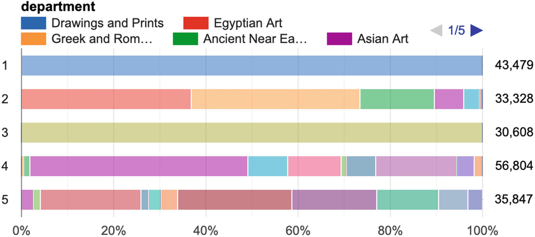
Visualization of k-means on types of art
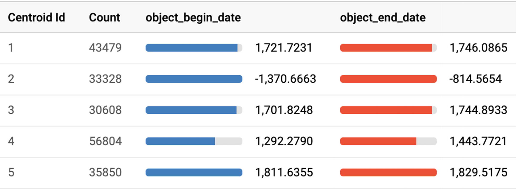
Numerical analysis of types of art by creation year
we see that the object dates for Cluster 2 are negative, as in BCE. So we have learned something—classical European art and drawings and prints are areas of focus for the Met’s curators, as is ancient art from all cultures. But—I hear you saying—we could have just sorted by prevalence and learned what the most popular categories are. What additional advantage does clustering give us here? Actually, if you look at a map of the museum,27 there are the fundamentals of a physical mapping here too.
Drawings and prints are only displayed for short amounts of time to avoid fading caused by exposure, so they have no fixed geographic location. Cluster 3 is mostly in the center of the museum, while Cluster 4 is found along the edges on the front and sides of the museum. Cluster 5 is in the back. Cluster 2 tended to represent antiquity across cultures and is also mostly located with Cluster 4.
So we can actually use this to propose, without any curatorial ability, a basic idea for how one might organize artwork in an art museum. Nonetheless, should I ever see a sign directing you to the K-Means Museum of Algorithmic Art, I’ll pass.
Evaluation and Prediction
K-means models return only two evaluation metrics, the Davies-Bouldin index and the mean squared distance. To improve your model, you want the index to be lower; changing the number of clusters to seek a lower score is one way to determine the optimal number of clusters for the data.
Sure enough, it recommends Cluster 1, with the rest of the drawings and prints, even though I made up and misattributed the department name.
Additional Exercises
The Met also publishes some additional tables, including a table with the results of the computer vision API run on each object. This includes intriguing assessments like whether the subject of the work is angry, joyful, or surprised. It also looks to identify landmarks, even going so far as to note their location. There are some interesting extensions to this model to cluster works by subject or location. (Spoiler alert: I added whether the subject was angry as a feature to this k-means model. It had no measurable impact.)
Data Classification
Data classification is a supervised model. BQML supports binary or multi-class, that is, yes/no or multiple categories. In this example, we’ll take a look at the National Highway Traffic Safety Administration (NHTSA) data for car accidents and develop a model for answering a question. Unlike k-means, where we went in a bit aimlessly, we have something in mind here. The question: If a car accident results in fatalities, given information about the accident and passengers, can we assess which passengers are likely to survive?
This may seem like a morbid question to ask, but it has significant ramifications in the real world. Regrettably, unfortunate accidents happen as a matter of course. Knowing which factors are associated with higher mortality rates can help at the macro level in provisioning emergency response levels and locations. It can characterize constellations of factors that may greatly increase the risk of fatality to improve car safety, road upkeep, or streetlight provisioning. It could even help on the ground directly—given partial information about the accident, it might suggest how quickly emergency services need to reach the scene and which passengers are at highest risk.
This model won’t do all of that, of course. It’s a jumping-off point intended to see how good it can get at answering the stated question, namely, can a given passenger survive a given accident, given that the assumption that the accident will cause at least one fatality.
Data Analysis
accident_2015: This carries the top-level data about the accident, including the time, location, and number of people and vehicles involved. It has one row for each accident.
vehicle_2015: This has information about each vehicle involved in an accident. It includes things like the type of vehicle and damage. It goes as deep as describing specifics of the vehicle’s stability before the accident, the area of impact, and the sequence of events.
person_2015: This has information about each person affected by the accident, including both passengers in vehicles, cyclists, and pedestrians. It includes demographic characteristics like age, the involvement of alcohol or drugs, and whether the passenger’s airbag deployed. It also has our target label, which is whether or not this person survived the accident in question.
Feature selection took quite some time in this example, given the vast array of data available. There are other tables describing driver impairment, distraction, the types of damage done, whether the driver was charged with violations, and hundreds more. This dataset would be suitable in building all kinds of regression and classifier models.
The last thing that will help if you really want to follow along in the details is the NHTSA Analytical User’s Manual28 (publication 812602). This has the full data glossary for all of the data points and will be extremely important as we perform feature extraction and transformation.
General: Where did the accident take place? What was the scene like? How were the roads? Was it day or night? What kind of road did it take place on?
Accident: What was the first thing that happened to cause the accident? Was it a collision and, if so, what kind?
Vehicle: What vehicle was involved for each passenger? Was it going the speed limit? Were there other factors involved? How serious was the damage to the vehicle? Did it roll over? How did the vehicle leave the scene?
Person: How old was the person? Where were they seated in the vehicle? Was the passenger wearing a seatbelt? Did the airbag deploy?
Response: How long did it take for emergency services to arrive? How long did it take to transport a person to the hospital?
This exploration took several hours to perform, so don’t assume it will be instantaneous to understand feature selection and extraction. Some features that I ultimately rejected included impact area (from 1 to 12 describing position on a clock), previous convictions for speeding, various personal attributes, maneuvers undertaken before the crash, and more than one descriptor for things like weather or extenuating circumstances. Many features helped only marginally or were eclipsed by other factors.
Creating the Model
For a model of this complexity, it makes sense to define the preprocessed data in a view as you go. That way you can see how it is developing and sanity-check any extraction you’re doing in the query selection. It also makes the model creation statement much cleaner. This is by no means necessary, but it’s useful to look at the input data you’re building without actually running the model over and over again.


All of the columns and their definitions
This statement generates the classification model by specifying the model_type as “logistic_reg” and the target label as “survived,” which is a column we defined in the view so that 1 represents a survival.
BUCKETIZE: This creates split points for categorical columns. These split points were determined by referencing the data dictionary and grouping common types together. For example, in the seating_position column, 10–19 are front row, 20–29 are second row, and 30–39 are third row. Rather than including all data about where precisely the passenger was sitting, this feature is extracted to convey only the row.
QUANTILE_BUCKETIZE: This represents values where ranges are useful but specific values are too granular. For example, we only care about the vehicle speed in increments of 10.
STANDARD_SCALER: This is used for columns where the relative value is more important than the absolute value. The exact time it takes for emergency services to arrive carries less weight than whether it is faster or slower than average.
When this statement is run, BQML gets to work and builds a model. This model takes several minutes to run and 17.6 MB of ML data. (Remember this is the statement that is billed differently than all of the other BigQuery statements.)
Evaluation
Once the model has been generated, we can review the statistics to see how it did.
When doing a binary classification model, BQML shows a slider for “threshold” allowing you to view the statistics for each threshold value. Recall that logistic regression is really a linear regression where you flip the decision from zero to one at a certain confidence threshold. To calibrate the model properly, we’ll decide which statistics we care most about and use that threshold for prediction. Open the model and click the “Evaluation” tab.
This model has a log loss of 0.5028. For equally weighted data, guessing neutrally for all instances, 0.5, would yield a log loss of ≈0.693. The probability of survival on a per-sample basis is more like 0.35, which means that a chance log loss should be lower than 0.693; however, 0.50 seems to intuitively indicate a decently predictive model. There are more advanced (not in BQML) analyses we could do like calculating the Brier score. Log loss is known as a somewhat harsh metric given that it penalizes confident inaccurate classifications so heavily.
The ROC AUC is 0.8149. This is quite good. It means that over all thresholds, the model is accurate for both positive and negative 81% of the time.
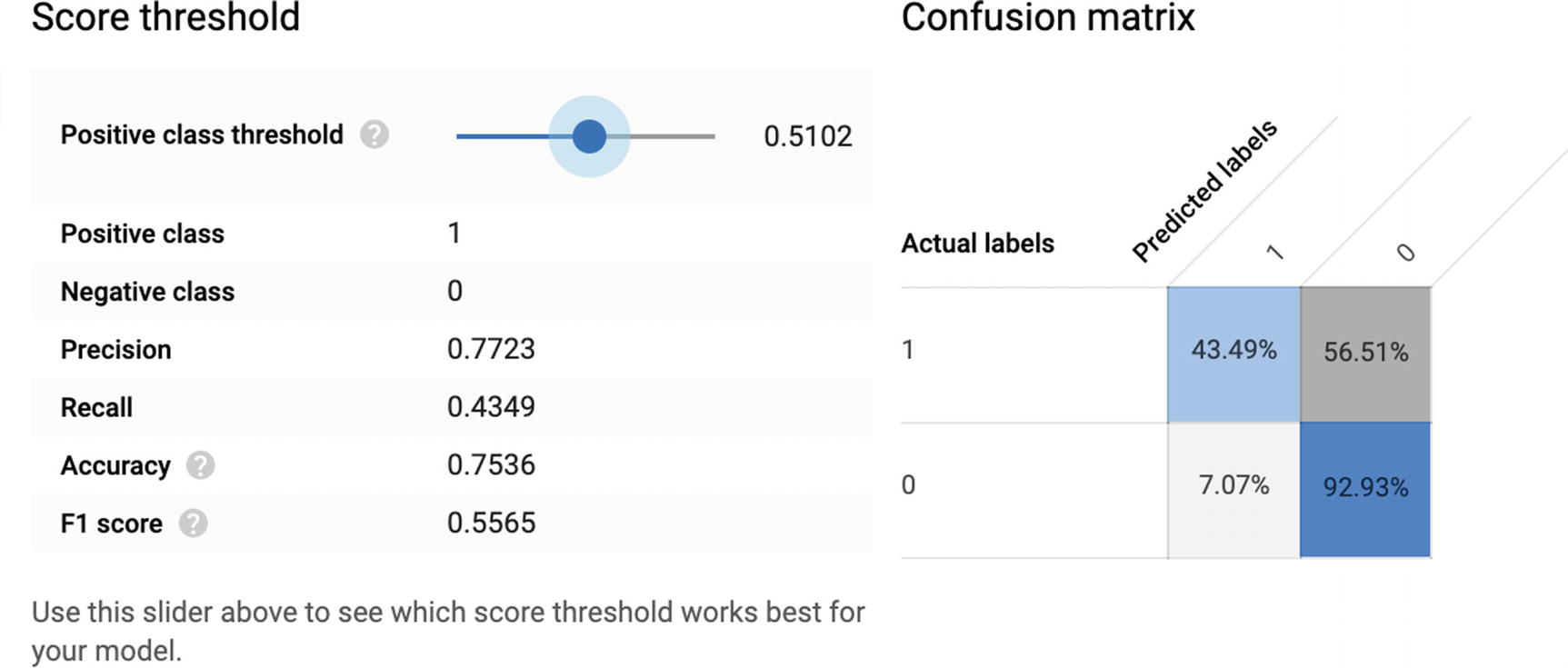
Model performance for a given threshold
At this threshold, the model correctly identifies 43% of all survivors and 93% of all fatalities and is right 75% of the time. Not bad. The F1 score, optimizing to both precision and recall, sits at a decent 55%.
Now we have to decide what we want to optimize for. Do we want to weight precision or recall more heavily? Do we want to find a balance of both, maximizing the F1 measure?
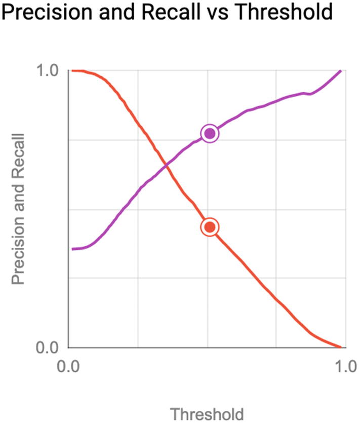
Precision and recall across all thresholds
Here, we see the expected tension between precision and recall. When the threshold is 0, that is, a positive prediction is never made, it’s always right, but that’s worthless. As the model begins selecting positive results more frequently, precision goes down and recall goes up.
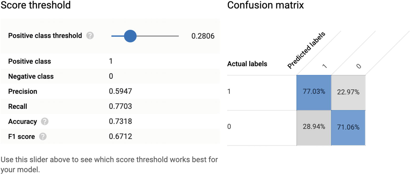
Threshold where the F1 score is highest
At a threshold of 0.2806, the model is accurate 73% of the time, correctly identifying 77% of survivors and 71% of fatalities. We sacrificed true negatives to increase true positives. The F1 score rises to 0.6712.
Overall, this model isn’t terrible. For a highly unpredictable event with so many variables, it’s actually a pretty good first pass. However, there are likely other correlating variables lurking deeper in the data, perhaps related to crosses of existing features, or more complicated extractions to amplify particular conditions. For example (and this is not based on the real data), traveling on certain types of roads in certain locations at certain hours of the week might drastically lower the probability of survival. In fact, some combinations might constitute outliers over the feature set and might be lowering the predictive model.
Prediction
We reserved an entire year’s worth of data to predict using our model. Let’s cut to the chase and try it out. This query manually constructs a confusion matrix from the 2016 results as a comparison, but also so that you can tinker with it to produce the other values.
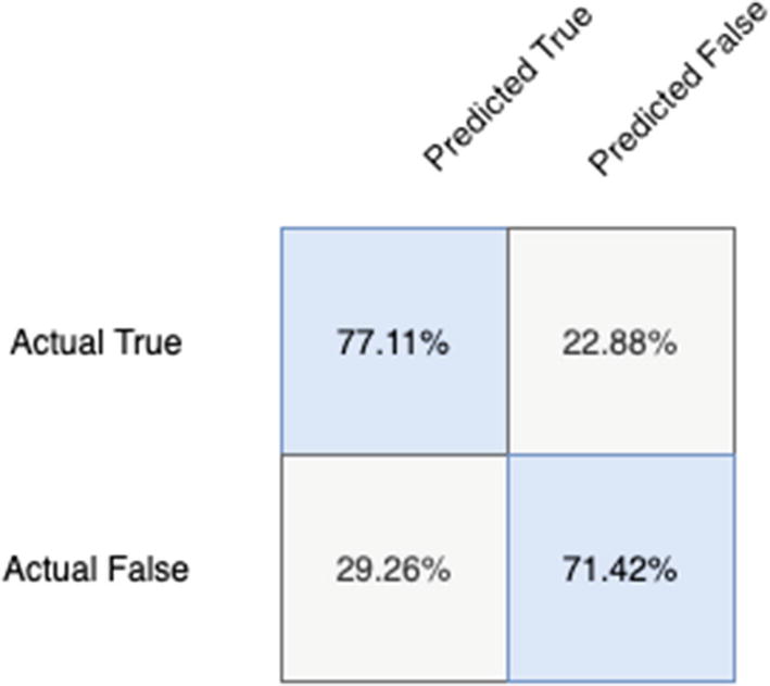
Confusion matrix for classification model
These results look almost the same, suggesting that this model retains the same predictive power from year to year. Two years is not a large enough sample, but in our nonscientific analysis, it’s encouraging to see the models line up so accurately.
Additional Exercises
A natural next step would be to do additional feature engineering. In my data exploration, pruning any single feature did lower max F1 and AUC slightly, but there must be better features to represent clusters of passenger or vehicle data. More feature extraction would yield a better understanding of outlier data, and removing outlier data could improve precision.
Are certain makes or models of cars more likely to be involved in fatal accidents?
Are cyclists more likely to be injured or killed by certain types of vehicles? Are adverse events like ejection correlated with mortality?
Are there physical characteristics that change mortality, like height and weight?
Does the behavior of the vehicle immediately prior to the accident matter?
Is previous driving performance actually a factor in the mortality rate associated with accidents? (My analysis was extremely limited and did not involve feature crossing.)
Can certain roads or highways be identified as especially dangerous? This one is huge—the road name, mile marker, and lat/lon of the accident are all available. Doing k-means clustering of the geography of accidents in a certain area might lead to some dangerous areas with much higher mortality rates. This in turn would be extremely useful to local authorities.
Hopefully this model has provoked some thoughts about the kinds of things even a simple binary classification can do. Are you excited yet? Go out there and do some exploration.
Summary
BigQuery ML, or BQML, is a feature intended to democratize machine learning for non-data scientists. Machine learning is a vast subfield of artificial intelligence and takes cues from statistics, mathematics, and computer science. However, it’s important to practice machine learning “for humans.” Interpretability and ethics of machine learning models are major considerations when using this technology. Using SQL directly in the UI, it is possible to process and train machine learning models in BigQuery. BQML supports both supervised and unsupervised models of several types, including k-means clustering, regression, and binary classification. Measuring the performance of each type of model is crucial to understanding its predictive power. The procedure for ML models is largely similar across types, involving preprocessing the data, creating the model, evaluating its performance, and then using it to make predictions. Through two examples, we saw the amazing power that even a simple model can produce—and a tantalizing glimpse of where it can go from here.
In the next chapter, we’ll explore the data science and machine learning community through Kaggle, Jupyter notebooks, Python, and their special integration into BigQuery. We’ll trade in mathematics for coding. You’re on your way to being a true student of machine learning!