17

Predictions: Diauxie, Electrons, Storage

This chapter links Part 1’s theory for biological design to Part 2’s problems of microbial metabolism.

The first section analyzes diauxie, the switch between alternative food sources. Microbes typically prefer some foods over others. The more strongly a cell focuses on a preferred food and represses the catabolic machinery for an alternative food, the longer it may take to switch to the second food after the first has been consumed.

How does temporal and spatial variation in food availability shape catabolic regulation? That question links metabolic design to theories of demography, life history, kin selection, and evolution in variable environments.

The second section considers the catabolic need for a final electron acceptor. Catabolic free energy comes from moving the weakly held electrons in food to strong electron acceptors, such as oxygen.

Finding an electron terminus becomes a primary catabolic challenge in the absence of oxygen or another abundant electron acceptor. Some microbes solve this challenge by transporting catabolic electrons to distant acceptors outside the cell.

Distributed electron flux raises many interesting problems of design. For example, some cells may produce extracellular electron shuttle molecules that carry electrons from the cell surface to a distant acceptor.

The extracellular shuttles, once released, may be used by neighboring cells. Such publicly shareable resources set many interesting design challenges. This section develops aspects of spatial scale and competition that arise for shareable public goods.

The third section evaluates cellular storage in complex life cycles. Cell lineages often pass through multiple habitats. Some habitats may lack food or final electron acceptors, preventing catabolism and requiring the use of stored free energy.

Building up and using resource stores often imposes tradeoffs. In a habitat that prevents catabolism, a bit more stored free energy used for growth means less available to maintain survival if the famine continues. The life cycle influences the relative costs and benefits for growth versus survival and thus for building and using storage.

This third section develops a wastewater treatment example that links alternating habitats and metabolic biochemistry to theoretical concepts of microbial design. Industrial microbiology provides many excellent models to study the forces that shape design.

The final section relates the particular models of microbial life history in this chapter to the broader problems of biological design. The primary challenge often concerns how to match the changes that we can study directly by observation or by dynamical models to the underlying forces that explain the motion, leading to Lanczos’ advice “to focus on the forces, not on the moving body.”²²²

17.1 Switching between Food Sources

Microbes often prefer particular foods (Section 14.5). For example, S. cerevisiae feeds first on glucose. It then shifts to feeding on other food sources, such as galactose.98,340

While feeding on a preferred sugar, cells that express catabolic genes for an alternative sugar may suffer reduced growth.⁴³⁷ In spite of that cost, pathway expression for the inferior food occurs in some cells.³⁴⁰

What forces shape mixed expression? This section illustrates how the core theory of Part 1 leads to comparative predictions.

PATCH LIFESPAN AND CYCLE FITNESS

Suppose a habitat divides into several isolated resource patches. Each newly formed patch contains an initial allocation of two sugars. No new sugar flows into an existing patch.

The first sugar provides a better food source for growth than the second one. How do design forces shape the pattern by which microbes consume the two food sources?

Comparatively, shorter patch lifespan favors high growth rate over efficient yield (Fig. 4.1). Intuitively, if a patch disappears before the resources are used up, efficient yield provides little benefit.

This age-specific force shapes how cells use the two different sugars. In this case, age means the time passed since a patch was colonized. Age-specific forces can often be analyzed by demographic cycle fitness (Section 5.7).

A simple model links catabolic regulation to cycle fitness. Existing patches die in each small time increment at a rate λ. New patches arise at the same rate. Each patch contains genetically homogeneous microbes, with genetic variation between patches.

In each time increment, migrants from existing patches colonize the new patches. All migrants to a new patch come from a single existing patch. The probability that an existing patch produces successful migrants is proportional to the current patch biomass, which measures population size and migration potential.

Demographic cycle fitness for a genotype is the sum, over all time increments of its patch’s lifespan, of the patch biomass at a particular time, b(t), multiplied by the probability of surviving to that time, t, as

$$w=\int b\left(t\right)\lambda e^{-\lambda t}\mathrm{\text{d}}t,$$

with average patch lifespan, 1∕λ. The caption of Fig. 17.1 describes the dynamics for the availability of the two sugars, the proteome expression levels for the pathways to catabolize each sugar, and the biomass.

The dynamics follows an intrinsic tradeoff between growth rate and biomass yield. Mechanistically, higher catabolic expression allocates more resources to increase growth rate, reducing resources available to produce biomass yield.

For each of four average patch lifespans, 1/λ = 1, 2, 4, 8, I maximized fitness subject to the rate-yield tradeoff mediated by catabolic expression level. In Fig. 17.1, the increasingly lighter shading of the curves corresponds to increasingly longer patch lifespans.

As patch lifespan increases, growth rate slows and biomass yield increases (Fig. 17.1a). In addition, the lag between consumption of the two sugars declines.

The catabolic expression levels explain the reduced lag (Fig. 17.1b). The top and bottom sets of curves show expression levels for the first and second sugar, respectively.

With longer patch lifespans, expression level for the primary sugar increases more slowly. Lower expression reduces growth rate, lowers the proteome cost for catabolism, and raises the biomass yield.

Proteome expression for the first sugar represses catabolic expression for the second sugar. As the expression level for the first sugar declines with longer patch lifespan, the catabolic expression for the second sugar rises.

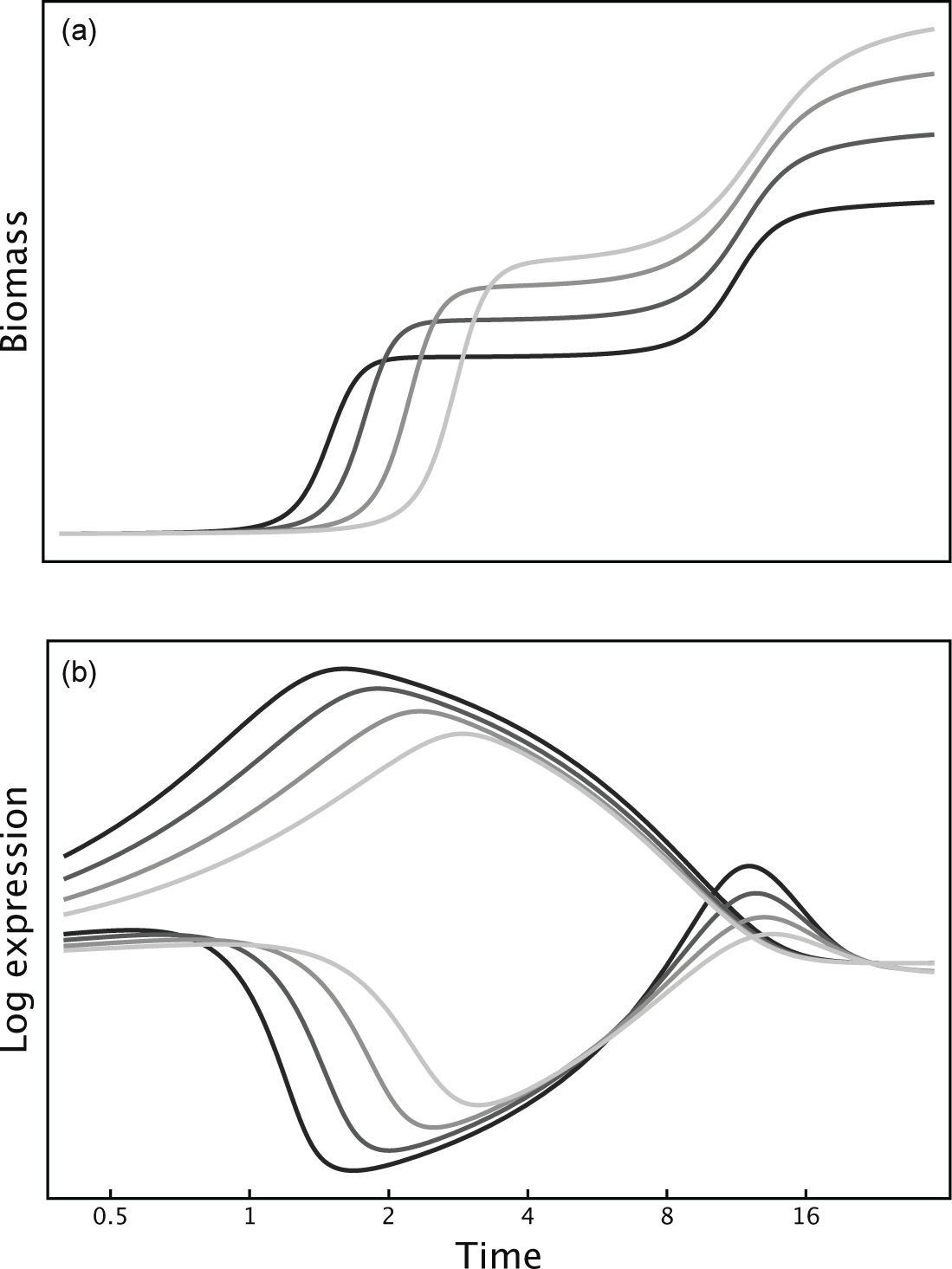
Figure 17.1   Patch lifespan alters the sequential consumption of two sugars. Average patch lifespan increases with lighter shading of curves. (a) Biomass change with time shows the growth rate during different periods of sugar consumption. (b) Expression level shows the proteomic allocation to the catabolic cascade. The top set of curves in this panel corresponds to expression for catabolism of the first sugar, the bottom set for the second sugar. See text for explanation of dynamics, which is given by the variables, x_i, y_i, b, for sugar concentration, proteome expression, and biomass, with i = 1, 2 for the first and second sugar, and tildes for initial values, with ${ẋ}_i=-x_i{y}_{i}b$, and ${ẏ}_i={\gamma }_i{x}_i{y}_i\left(f-y_i/5\right)+\left({ỹ}_i-y_i\right)/2-c_i{y}_1{y}_2$, and $ḃ=b\left(x_1{y}_1+0.9x_2{y}_2\right)\left(1-f\right)$, with ${\gamma }_1=1,{\gamma }_2=0.35,c_1=0,c_2=12,r_1=1,r_2=0.9,{\tilde{x}}_i=10,{ỹ}_i=0.01,\tilde{b}=0.1$, . The value of f maximizes fitness, calculated by ${\int }_0^{30}b\left(t\right)\lambda e^{-\lambda t}\mathrm{\text{d}}t$ for average patch lifespans 1/λ = 1, 2, 4, 8. This model extends Frank’s130 analysis for a single resource.

During the initial feeding on the first sugar, greater expression for the second sugar reduces the lag between growth on the two sugars.

Empirically, two key puzzles of sequential sugar usage often arise. Why is significant expression level for the second sugar sometimes maintained during consumption of the first sugar? What explains variability in the lag time between growth on the first and second sugars?

Testable comparative predictions follow from the simple patch lifespan model. For example, increasing patch lifespan emphasizes yield over rate, which favors a more balanced catabolic expression for the two sugars and shorter lags between growth on alternative food sources.

COMPETITION AND RELATEDNESS

Figure 17.1 assumes a single type in each patch. If the types mixed and competed within patches, that competition would favor faster growth and lower yield (Section 4.1).

The relatedness between competitors measures the intensity of competition (Section 5.2). The more mixing of types during patch colonization, the lower the relatedness and the more intense the competition between different types for local resources.

How does increasing competition between types affect the consumption of multiple resources? Chapter 5 provides the concepts to analyze relatedness and demography. I limit comments here to likely comparative tendencies based on a simple qualitative approach.¹³⁰

Lower relatedness and greater competition favor faster growth rate and reduced biomass yield. In Fig. 17.1, decreasing relatedness has a similar effect to shorter patch lifespan (Fig. 4.1).

The benefit of faster growth alters the regulation of sequential resource consumption. The particular change depends on the tradeoffs imposed by the mechanistic basis of regulation.

The commonly studied lab species are often tuned for competition and fast growth. By contrast, natural environments vary widely in demography and relatedness. Broad comparative changes likely occur.

Figure 17.2   Reduced proteome limitation allows higher catabolic expression for a second food source, shortening the lag time for the switch between food sources. Same model as in Fig. 17.1, with c₂ = 2 to reduce the repressive effect of catabolic expression for the first food source on the expression level for the second food source.

PROTEOME LIMITATION

In Fig. 17.1b, catabolic expression for the first food strongly represses expression for the second food. Repression may arise because of proteome limitation, which imposes a tradeoff between catabolic protein expression for the alternative foods.

What happens under reduced proteome demand, which weakens the tradeoff between catabolic expression for alternative foods?

To study that question, Fig. 17.2 analyzes the same model, with a reduced intensity for the repressive effect of the catabolic proteins for the first food on the catabolic expression for the second food.

Figure 17.2b shows that less intense proteome limitation allows maintenance of greater catabolic expression for the second food source while consuming the first source. That greater expression reduces the lag time between growth on the alternative food sources (Fig. 17.2a).

As always, this comparative prediction describes a partial causal effect. Reduced proteome demand may also affect other causes. Those other causes may alter the net effect on catabolic expression.

If so, then reduced proteome demand may sometimes fail to increase the catabolic expression for the second food source. However, the tendency over different cases should be in the predicted direction.

UNPREDICTABLE RESOURCE INFLUX

The prior examples assumed that each resource patch starts with a fixed amount of the two alternative sugars. What if the temporal and spatial patterns of resource flux vary? Six simplified scenarios highlight important partial causes (Section 5.10).

Environmental fluctuations favor catabolic expression that buffers against variability in performance.—Suppose the environment divides into many separate patches. Each patch contains a single genotype. At the start of each of n identical time intervals, a random amount of each sugar arrives and is split equally among the patches.

After the final time interval, all patches contribute migrants to a global pool. Each patch contributes migrants in proportion to its final population size.

The current patches disappear. New patches arise. One genotype colonizes each new patch. A genotype’s frequency in the migrant pool determines its colonization success.

In this scenario, what pattern of catabolic expression improves success? To answer, we must consider the sequence of growth in each patch in response to the random influx of additional sugar.

Suppose population size in a patch increases by a multiplicative factor λ_ij in time interval i for genotype j. Total reproductive yield for genotype j over a complete demographic cycle is the product of the λ_ij values over the sequence of time intervals (Section 5.10).

A multiplicative product of values scales with the geometric mean of those values. Thus, the total-yield measure of fitness over a complete demographic cycle scales with the geometric mean of growth values over the sequence of time intervals.

In terms of regulatory control, the forces of design favor catabolic expression for the two sugars that increases geometric mean growth. The geometric mean rises with the arithmetic average of the interval growth values, λ_ij, and declines with variability in those values.

Comparatively, more variable mixtures of sugars often favor more balanced catabolic expression. Balanced catabolic expression enhances the geometric mean growth when the gain for reducing the variability in growth outweighs the loss for reducing the arithmetic average.

For example, more variable resource influx will sometimes present cells with a relatively high amount of the less preferred sugar. To prevent low efficiency because of unused high expression for the preferred sugar, cells may tend to balance their initial expression for the two sugars.³⁸⁰

That bet-hedging³⁸⁶ between alternatives relates to timescale. The highest geometric mean maximizes the expected growth rate over the full demographic cycle. A higher expected success over the full cycle may associate with lower success in particular intervals of resource influx. Spatially correlated variability and global competition.—In the prior example, the final population size of each patch is the product of growth during each episode of resource influx. That multiplication of periodic growth leads naturally to a geometric mean measure of fitness. After several episodes of local resource influx and growth, migrants mix and recolonize new patches.

An alternative demographic cycle may occur. New patches form, each containing the same mixture of the two sugars. The particular mixture varies at the start of each cycle. Microbes grow by consuming the initial sugar allocation. Following a period of growth, the microbes disperse, mix globally, and colonize new patches.

Suppose there are two genotypes. A focal genotype has frequency q. The alternative has frequency 1 − q. After one cycle, the frequency of the focal genotype is

$$q^{\prime }=\frac{w_{1}q}{w_{1}q+w_2\left(1-q\right)},\text{(17.1)}$$

in which w₁ is the multiplicative fitness factor by which the focal genotype increases its population size during its period of growth within its patch, and w₂ is the fitness for the alternative genotype.

Because the resource mixtures vary over time, the fitness values will also vary. As in the prior scenario, we assume that the different genotypes have different patterns of catabolic regulatory expression for the alternative sugars. Those different expression patterns cause differences in fitness between the genotypes.

Once again, the favored genotype has the highest geometric mean for its temporal sequence of fitness values. For example, suppose the resource influx has two equally probable states with fitnesses w₁ = 1 ± δ and w₂ = 1 ± (δ + 𝜖), with δ, 𝜖 > 0.

The arithmetic average fitness for both genotypes is 1. The geometric mean fitness is greater for w₁ because of its lower variability in fitness values. The genotype with the higher geometric mean fitness increases against the alternative genotype.^80,144,153

A genotype with a lower arithmetic average fitness can increase if its fitness varies less between environments, leading to a higher geometric mean. If, between two environments, w₁ = 1 for both environments and w₂ = {0.82, 1.2} for the two environments, then the arithmetic and geometric means for w₁ are both 1, and for w₂ are 1.01 and 0.992.

In this case, the first genotype typically increases in frequency because it has the higher geometric mean fitness, in spite of its lower arithmetic mean fitness. Using eqn 17.1 with an initial frequency of q = 0.5, after one episode of each environment, q = 0.504.

Dominance of the geometric mean implies that genotypes may gain by trading a reduced arithmetic mean success for a reduced variability in success across environments.

Comparatively, the more variable the environment over time, the more strongly catabolic regulation may trade reduced arithmetic success for reduced variability in success.

Spatially uncorrelated variability and global competition.—In the prior examples, resources flow into each patch in the same way. Alternatively, resource flows may be uncorrelated between patches.

If much of the variability in resource flows occurs spatially, then a genotype experiences nearly all of the alternative environments in each time period. The total contribution of that genotype to the migrant pool at the end of the growth cycle depends on the arithmetic average success over the different spatial environments.

If arithmetic average success over spatial patches varies little over time, then the geometric mean success of the genotype over time is very close to the arithmetic average over space.

Comparatively, the more weakly correlated resource flows are between patches and the more closely the spatial distribution matches the temporal distribution of patch characteristics, the more strongly the arithmetic mean will dominate over the geometric mean.

The particular catabolic expression patterns that maximize arithmetic versus geometric mean success depend on the details. Typically, the geometric mean favors reduced variability in success.

Thus, less spatial correlation implies greater dominance by the arithmetic mean, less emphasis on reducing variability in success, and less bet-hedging in the expression of catabolic regulation.

Stochastic gene expression reduces spatial correlation.—Catabolic expression may vary stochastically between individuals of the same genotype.³⁸⁰ Such variability can reduce the spatial correlation in fitness.

Lower correlation between individuals tends to reduce the variability in genotype success. Lower variability raises the geometric mean.

Comparatively, increased environmental variability favors greater stochasticity in gene expression to reduce genotypic variability and raise geometric mean fitness.

That comparative prediction highlights a partial causal effect. The particular details influence the overall value of stochastic variability.

Local competition for colonization and rare-type advantage.—Prior examples emphasized spatial correlations in environments and in trait expression between individuals. Spatial properties define demographic aspects of populations.

This example focuses on the spatial scale of competition, another key demographic property. As before, suppose that each patch begins with a single genotype and a random allotment of the two sugars. Cells consume the sugars and increase their population. A migrant pool forms, colonizes new patches, and repeats the cycle.

In prior examples, all new patches receive their colonists from a global migrant pool. In this example, the global set of patches divides into many distinct regions.

Each region forms its own migrant pool, which then colonizes only the newly formed patches in the local region. Occasionally, a global cycle of migration and colonization occurs. Most of the time, competition for colonization happens locally within regions.

Comparatively, greater local competition increases the amount of genetic variability maintained in the global population.

That increase in genetic variability occurs because environmental fluctuations favor rare types. Equation 5.19, repeated here, illustrates the rare-type advantage,

$${\mu }_1-q_1{\rho }_1{\sigma }_1^2>{\mu }_2-q_2{\rho }_2{\sigma }_2^2.$$

The two competing genotypes, with subscripts i = 1, 2, have arithmetic fitness means, μ_i, frequencies, q_i, fitness correlations between individuals of the same genotype, ρ_i, and variances in fitness, ${\sigma }_i^2$.

This expression describes the conditions for genotype 1 to gain against genotype 2, assuming that fitness fluctuations are small and the correlation between genotypes is zero.

The smaller a genotype’s frequency, q_i, the less the overall fitness discount that arises from the variability in success, ${\sigma }_i^2$. That rare-type advantage tends to maintain genetic variability. For example, if we assume equal arithmetic means and equal correlations, then overall fitnesses in the above expression become equal when

$$\frac{q_1}{q_2}=\frac{{\sigma }_2^2}{{\sigma }_1^2}.$$

Less variability in success increases the equilibrium frequency of a genotype.

However, when competition occurs in a single global population, fluctuations in frequencies often cause extinction of the genotype with more variable success. Ultimately, the less variable genotype tends to dominate the global population.

By contrast, when competition for colonization happens locally across many separate regions, the global frequencies arise by averaging over the local regions. Averaging many independent local events lowers the global fluctuations. With lower fluctuations in frequencies, the equilibrating tendency of the rare-type advantage dominates, maintaining genetic diversity.

Local competition for resources.—The prior examples assumed a single genotype in each isolated resource patch. Mixing genotypes in patches would impose local competition for resources. Such local competition typically favors higher growth rate at the expense of reduced yield.

With regard to variable environments, within-patch competition alters how patterns of catabolic expression affect arithmetic mean fitness and the fluctuations in fitness. Mixtures within patches also induce correlations between genotypes with regard to environmentally caused fluctuations in fitness.

It would be interesting to develop theory that combined direct competition between genotypes and spatially induced correlations in fitness. Both causal paths influence the favored patterns of catabolic expression.

17.2 Distributed Electron Flux

Catabolism generates free energy by passing electrons through a redox gradient. Roughly speaking, the initial food source holds electrons relatively weakly. The final electron acceptor holds electrons relatively strongly. The electron gradient flows from low to high entropy or, equivalently, from high to low free energy.467

The catabolic free energy potential depends on the strength and availability of the final electron acceptor. Finding a strong, renewable receptacle for electrons forms a primary challenge of metabolism.

Many organisms pass electrons to oxygen, the basis for aerobic respiration. Some habitats lack sufficient free oxygen. Alternative electron acceptors create broad metabolic diversity in microbes.

Electron flux typically happens between coupled biochemical reactions within cells. However, some microbes move free electrons from donor molecules to spatially distant receptor molecules, creating an extracellular electric current (Section 14.4).

CABLE BACTERIA

Cable bacteria transmit electric currents across thousands of connected cells.²⁷⁷ The current passes electrons to oxygen or nitrate. The terminal cells act solely as conduits, failing to grow.¹⁵¹

Cooperation between the connected cells and the reproductive sacrifice of the terminal cells pose interesting puzzles (p. 225). Before turning to those puzzles, I briefly review the biology (p. 213).

Genomic analysis suggests a broad array of catabolic pathways in cable bacteria.^210,289 A particularly interesting catabolic cascade follows two steps. First, in a habitat without free oxygen, cells feed on hydrogen sulfide by splitting that molecule with water to make sulfate, free protons, and free electrons (eqn 14.2).

Second, multiple cells physically link to form a cable that stretches from the anoxic zone to a region that has free oxygen.^{151,152,210,368} Electrons flow along nickel-protein wires in the cellular periplasmic space between the inner and outer membranes, creating an electric link from the anoxic zone to the oxic zone.⁴⁵ At the oxic terminal, the incoming electrons combine with oxygen and protons to make water (eqn 14.3).

More than 90% of the cells reside in the anoxic zone. The remaining nonreproductive cells in the oxic zone act solely as wires that conduct electrons to the oxic region. Why would the oxic cells act altruistically, providing a benefit to the anoxic cells without gaining any growth benefit for themselves?¹⁵¹

The unusual natural history raises other questions. How do the cables form and grow? Do long cables sometimes split into smaller cables? If so, how do the buds compete with each other spatially? How do the bacteria colonize new resource patches?

Limited empirical information prevents convincing comparative predictions. However, more observations will soon follow because cable bacteria occur widely in aquatic sediment and may play a key role in geochemical cycles.^{53,248,342,361}

I first summarize the details of metabolism and the life cycle. From that sketch of the natural history, I then consider the forces that may shape metabolic design. Compelling puzzles of microbial life history arise.

Altruistic oxic terminal cells.—Cells in the oxic zone do not assimilate carbon and do not divide.^151,152 The rapid electron influx typically reduces oxygen to water, perhaps causing strong oxidative stress.^210,368

Oxic zone cells are likely related to their connected cable partners by recent cell divisions, causing high genetic similarity between cells in a cable. That high genetic similarity provides the most likely explanation for the oxic cells’ sacrifice of their own reproduction to benefit their anoxic partners (Section 5.2).

Other processes may explain oxic cellular sacrifice. Alternatives include randomization with regard to their role as contributor to or recipient of benefits to neighbors, synergistic fitness benefits between partners with low relatedness, and positive ecological feedback.¹²⁶ However, initial focus should be on the simple explanation of high relatedness before considering more complex processes.

The forces that shape cable bacteria altruism and life history depend on how cables form, grow, compete, and disperse. A few limited studies provide initial observations.

Cable growth, cell number, and length.—Geerlings et al.¹⁵² observed cable growth in the lab. Cables grew rapidly when connected to both the anoxic electron source and the oxic electron sink. Loss of contact at one terminal stopped growth.

Cell length is approximately 2–3 µm.^259,354 Cable length increases up to a few cm, with about 4000 cells cm⁻¹.

Movement.—Bjerg et al.⁴¹ observed cable movement in slide preparations. The center of the slide contained anoxic sediment. Slide edges provided an oxic interface. Cables actively moved toward the oxygen boundary. The leading filament tended to stop when in contact with the oxic zone. As the oxygen boundary moved, cables followed.

Cables may elongate from an oxic zone boundary down into the anoxic sediment. Cables are relatively straight near the oxic boundary. Cables may coil into a terminal snorkel toward the sulfide electron source.^354,462

Population density.—Schauer et al.³⁵⁴ collected deep sediment, likely below the zone at which cables could connect to the oxic zone. They incubated the sediment with the upper layer exposed to oxygen. The initial cable bacteria density was below their threshold detection for cables at 10⁴ filaments cm⁻³ or, for single cells, at 1.5 × 10⁶ cells cm⁻³.

At initial incubation, anoxic-zone sulfide occurred within 1 mm of the anoxic-oxic interface. After 10 days of incubation and consumption by the growing cable bacteria, most sulfide retreated to a boundary 2–8 mm below the oxic zone, dropping to 20 mm by day 53.

In the 0–15 mm depth interval, at 10 days, the cable bacteria density in each cm² increased to approximately 1 km of cables. At 21 days, density per cm² approximately doubled to over 2 km, or about 8 ×10⁸ cells cm⁻³.

Habitat heterogeneity and fragment length distribution.—Various physical and biotic processes perturb sediments. Disruption may break bacterial cables, preventing growth.²⁵⁹ Disruption may also create new opportunities to link anoxic sulfide zones to oxic zones.

For example, parchment worms build tubes into the sediment, creating novel oxic zones. Abundant cable bacteria occur near those tubes. The tubes can be structurally stable for several months.⁸

Measured cable lengths near tubes were up to 1 mm, approximately 400 cells. A few mm away from tubes, measured cable lengths tended to be 5–15 cells. However, this study’s measurement methods could not rule out fragmentation during sample processing.⁸

Overall, the size distribution of unconnected cables remains an open problem. A recent lab culture found single cells and short cables in a growing population²⁸⁹ (see below).

ATP generation.—Overviews of cable bacteria metabolism typically emphasize the half reactions in eqns 14.2 and 14.3, repeated here,

$$\begin{array}{lll}\hfill {\mathrm{H}}_2\mathrm{S}+4{\mathrm{H}}_2\mathrm{O}& \to {\mathrm{SO}}_4^{2-}+8{\mathrm{e}}^{-}+10{\mathrm{H}}^{+}& \hfill \text{(17.2a)}\\ \hfill 2{\mathrm{O}}_2+8{\mathrm{H}}^{+}+8{\mathrm{e}}^{-}& \to 4{\mathrm{H}}_2\mathrm{O}.& \hfill \text{(17.2b)}\end{array}$$

The first reaction, in the anoxic zone, hydrolyzes hydrogen sulfide. The generated electrons flow to the oxic zone through bacterial cables, and the protons flow extracellularly over the pH gradient. The second reaction, in the oxic zone, combines the influx with oxygen to make water. Variant reactions occur. For example, nitrate may be used instead of oxygen as the electron acceptor in the second reaction.

These reactions focus on the flow of electric current. But they leave open three questions. How do cells generate ATP to drive growth? Can cables grow when not connected across habitats? How do single cells grow when alone?

The following discussion fills in background. The background includes significant biochemical detail. The effort to follow that detail is repaid when we arrive at a hypothesis for the cable bacteria life cycle. That life cycle presents a fascinating challenge for understanding microbial life history and the forces that shape metabolic design.

Genomics provides the first piece of the background. Cable bacteria genomes encode diverse metabolic processes. Two studies found genes for ATP-generating pathways on alcohols, hydrogen, and sulfur compounds. The genomes from marine210 and groundwater²⁸⁹ habitats differed with regard to the presence of particular genes.

ATP from elemental sulfur and growth of single cells.—Müller et al.²⁸⁹ developed a hypothesis for how cable bacteria generate ATP from sulfur. Their model arose from culture under different conditions, in which they grew cable bacteria obtained from groundwater.

In one culture, elemental sulfur was the only electron donor source. That growing culture did not favor significant electron flux over cables, suggesting ATP generation and growth in the absence of electron flux.

The culture contained single cells and cables up to several hundred µm in length. As populations grew, they seemed to contain longer cables and more cables relative to single cells. This culture suggests that single cells may grow into populations with small cables.

Growth on elemental sulfur required an additive that scavenged sulfide. When comparing the classic summary of cable bacteria metabolism and electricity in eqns 17.2, it is not immediately clear why the only sulfur-related requirements for growth are adding elemental sulfur, S⁰, and removing sulfide, S^2–, which may occur as H₂S or HS^–.

Many bacteria, including species closely related to cable bacteria, use S⁰ as their electron-donor source of free energy.^105,289 The cable bacteria genome analyzed in this study contained the necessary genes for that elemental sulfur pathway.²⁸⁹

For example, an overall transformation may be¹⁰⁵

$$4{\mathrm{S}}^0+4{\mathrm{H}}_2\mathrm{O}\to {\mathrm{SO}}_4^{2-}+3{\mathrm{HS}}^{-}+5{\mathrm{H}}^{+}.\text{(17.3)}$$

Dropping the protons simplifies the reaction to

$$4{\mathrm{S}}^0+4{\mathrm{O}}^{2-}\to {\mathrm{SO}}_4^{2-}+3{\mathrm{S}}^{2-}.\text{(17.4)}$$

The unusual biochemical aspect arises because the transformation happens by a combination of two coupled redox reactions,

$$\begin{array}{lll}\hfill {\mathrm{S}}^0+4{\mathrm{O}}^{2-}& \to {\mathrm{SO}}_4^{2-}+6{\mathrm{e}}^{-}& \hfill \text{(17.5a)}\\ \hfill 3{\mathrm{S}}^0+6{\mathrm{e}}^{-}& \to 3{\mathrm{S}}^{2-},& \hfill \text{(17.5b)}\end{array}$$

in which S⁰ is the electron donor in the first oxidation reaction and the electron acceptor in the second reduction reaction. This disproportionation of sulfur105 may be summarized as

$${\mathrm{SO}}_4^{2-}\leftarrow 4{\mathrm{S}}^0\to 3{\mathrm{S}}^{2-}.\text{(17.6)}$$

The left-side oxidation of sulfur to sulfate can produce ATP, providing the free energy disequilibrium to drive growth.

Figure 17.3   Increasing sulfide (HS^–) concentration stops metabolism of S⁰ by product inhibition, raising the free energy change above zero. Dotted line shows the threshold. The reaction summarizes the sulfur-disproportionation pathway in eqns 17.3–17.5. Theoretical calculation at 4 °C and 28 mM ${\mathrm{SO}}_4^{2-}$. Higher temperature (25 °C) or less sulfate (3 mM) roughly doubles the sulfide threshold for the reaction to proceed. Redrawn from Fig. 1 of Finster.105

A buildup of sulfide inhibits this metabolic pathway. Figure 17.3 shows that increasing sulfide concentration blocks the reaction.

The sulfur cycle.—One study²⁸⁹ showed that cable bacteria can grow on S⁰. How does that relate to the commonly cited pathway for generating electron flux in eqn 17.2a, which begins by uptake of sulfide, S^2–?

Figure 17.4 provides a model for local sulfur cycling, ATP generation, and electron flux over cables.

In that model, all suboxic cells can oxidize sulfide to sulfur, S²⁻ → S⁰ + 2e⁻, which does not generate ATP. The electrons flow up the cable to the oxic zone to reduce oxygen to water.

When the sulfide concentration is sufficiently low, suboxic cells disproportionate sulfur into sulfate and sulfide, as in eqn 17.6. The ${\mathrm{S}}^0\to {\mathrm{SO}}_4^{2-}$ pathway generates ATP.

Cells excrete ${\mathrm{SO}}_4^{2-}$. Sulfate-reducing bacteria are common.¹⁹⁷ They use essentially the same reactions as disproportionation but, compared with eqn 17.6, they run the sulfate-sulfur reaction in reverse,

$${\mathrm{SO}}_4^{2-}\to {\mathrm{S}}^0\to {\mathrm{S}}^{2-},\text{(17.7)}$$

which regenerates sulfide and completes the local cycle.

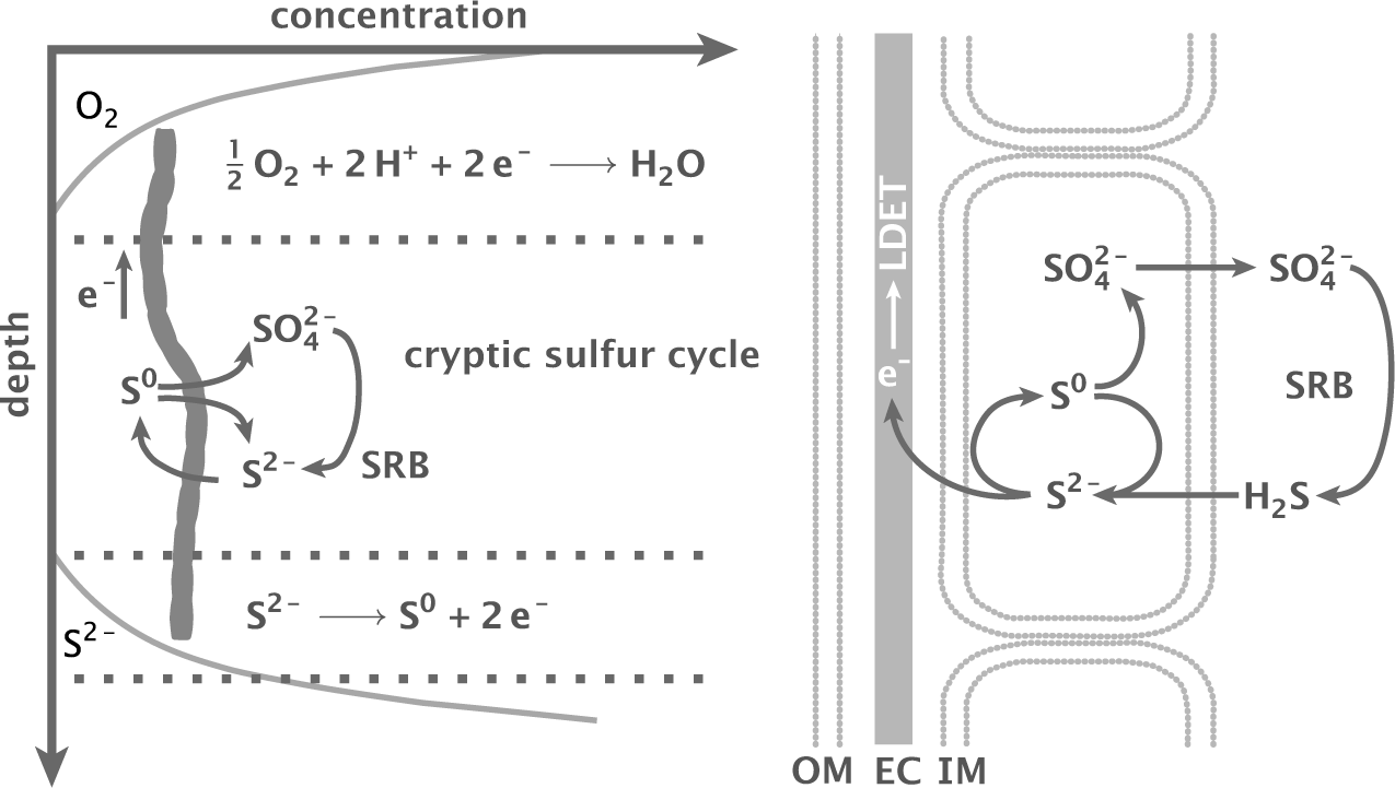
Figure 17.4   Model for sulfur cycling by cable bacteria and sulfate-reducing bacteria (SRB). See text for the steps in various pathways. The cells on the right show the inner membrane (IM), outer membrane (OM), and electron cable (EC) over which long distance electron transport (LDET) runs. Redrawn from Fig. 4 of Müller et al.289

The overall model in Fig. 17.4 distinguishes three zones. First, the upper zone uses the incoming electrons to reduce oxygen or nitrate.

Second, the middle zone runs a complete sulfur cycle. Cable bacteria take up sulfide and produce sulfate. The sulfate-reducing bacteria transform sulfate into sulfide. Little net change may be observed. That apparent stasis misleadingly suggests limited metabolic activity.

Third, near the anoxic cable ends, sulfide concentration may rise because the cable bacteria do not take it up sufficiently quickly. High sulfide concentration blocks the ATP-generating sulfur disproportionation pathway. Thus, the anoxic ends may act as nongrowing sulfide oxidation uptake terminals, passing their electrons up the cable.

This model completes the summary of metabolism and the life cycle. With that background, I turn to the forces that shape life history.

Habitat niche construction.—In the sulfur-cycle model, high sulfide concentration inhibits the sulfur disproportionation pathway (eqn 17.6) that provides ATP for growth. A nongrowing cable terminal, down in a sulfide-rich zone, could lower the sulfide concentration by oxidation,

S²⁻ → S⁰ + 2e⁻,

sending the electrons up the cable and raising the nearby S⁰ concentration (Fig. 17.4). Once the sulfide concentration drops sufficiently, the pool of S⁰ provides food for growth. S⁰ may also diffuse upward into the active growth zone, providing additional food to enhance reproduction.

This niche construction³⁰² process makes the habitat better for growth. A cable that improves the habitat for itself also improves conditions for neighboring cables.

Put another way, lowering the sulfide concentration by electron conduction over the cable provides a shareable public good for neighbors. The neighbors include connected cells attached to the same cable and the many separate cables that likely reside nearby.

The extensive theory for public goods evolution applies. That theory leads to a wide variety of comparative hypotheses in relation to demography and the genetic structure of populations (Chapter 5).

Most simply, greater genetic relatedness typically favors more investment in public goods. In this case, separate cables with more closely related cells are more likely to improve high sulfide environments in a way that benefits all neighbors.

Demographically, long-lived patches typically gain more from niche modifications than short-lived patches.

Tuning of rate versus yield.—Initial studies tend to focus on habitats with high bacterial density. It is easier to find and observe a lot of bacteria than it is to study sparse populations.

High density often associates with genetic mixing. More mixing favors faster growth rate at the expense of reduced yield (Section 4.1).

Isolated resource patches inevitably come and go. Such patches often contain more highly related populations, which tend to favor greater yield and reduced growth rate. Patch lifespans and rates of resource influx also vary, altering the forces that favor rate versus yield.

Demographically, short-lived patches typically favor faster growth. Long-lived patches with limited resources typically favor higher yield.

Those abstract forces apply widely across microbes. It would be particularly interesting to study the mechanisms by which those forces tune the unusual metabolism of cable bacteria.

The scale of competition and dispersal.—Public goods and high yield provide cooperative benefits to neighbors, enhancing group success. High relatedness typically favors those cooperative traits. However, if neighbors also compete for resources, that competition can offset the benefits and disfavor the cooperative traits (p. 72).

Demography plays a role. For example, public goods, such as beneficial niche construction, may affect close neighbors. By contrast, competitive interactions, such as dispersal and colonization of new patches, may happen between distant competitors.

Comparatively, the more intensely cooperation happens locally between close relatives and the more intensely distant competition happens globally against unrelated individuals, the more strongly natural selection will favor cooperative traits.¹²²

Spatial scaling of cooperation and competition depends on movement. Cables actively move, as summarized above. Movement may primarily serve to maintain electron flux between anoxic and oxic zones.

Additional movement in excess of what is needed to maintain electron flux may occur in order to increase dispersal distance, reducing competition between close relatives. Comparatively, more local competition between relatives favors greater excess dispersal.^111,169

Budding and breakpoints in the formation of new cables.—As cables grow, they must eventually break into smaller pieces. Those buds are the cables’ progeny.¹⁵⁰

A long cable could produce many single cells and short cables. Or it could break near the middle, making fewer large buds. Demographically, the number of offspring trades off against the size per offspring.³⁸⁷

Changing conditions alter the relative reproductive value of small and large offspring (Section 5.6). For example, short-lived resource patches favor dispersal, which likely values many small progeny more highly than a few large progeny.

By contrast, a strong growth premium for cables that connect anoxic to oxic zones likely values a few long progeny over many short ones.

Mechanistically, the breakpoint tendency between various cells may evolve in response to changing design forces on progeny size.

Many aspects of resource distribution, demography, and genetic structure influence the design forces that favor different-sized offspring. I leave the development of comparative predictions as an open challenge.

Hookups between cables.—Can a suboxic cable dump excess electrons by physically connecting to a cable with an oxic terminal? There are a few clues but no direct evidence.

Reimers et al.³³⁸ placed a carbon electron-accepting anode into river estuary sediment. After 412 days, they found cable bacteria filaments of more than 40 cells firmly attached to the electrode. Presumably, the short filaments in the anoxic habitat dumped their excess electrons through their physical connection to the electrode.

Competitive habitats may favor hookups between cables. Linking cables increases the rate at which short filaments can span zones to transmit electrons. Interspecies links may bring synergistic metabolic pathways into proximity, allowing joint exploitation of new resources.²⁵²

EXTRACELLULAR ELECTRON SHUTTLES

Other microbes transmit electrons extracellularly. This subsection focuses on shuttle molecules that pick up electrons at the cell surface, move by diffusion, and dump the electrons on a distant recipient.

Those freely diffusing shuttle molecules can potentially be used by any nearby cells. Some cells may not make any shuttles, instead using the shuttles made by other cells.

The public goods problem arises when a cell produces a shareable resource that diffuses away and can be used by any neighbor (Chapter 5). The producer pays the cost. All neighbors can benefit.

The overall costs and benefits of diffusible shuttles depend on the molecular mechanisms, the similarity or relatedness between neighbors, and demography.

Thermodynamic background.—Catabolic cascades move electrons from donor molecules to recipient molecules. Donor molecules provide food. Recipient molecules provide an electron sink.

Electrons come from food, pass through the catabolic cascade, and must be dumped after use. The thermodynamic driving force depends on electron flux through the full path. Cells fuel life by capturing free energy from that electron flux.

For microbes that can access and use oxygen, finding an electron sink provides little challenge. For microbes in anaerobic conditions, accessing a good electron sink may be just as challenging as obtaining food.

In some cases, the internal catabolic cascade provides the final electron sink. For example, the molecules that accept electrons to make acetate may be the final electron sink for anaerobic fermentation.

Often a cell must dump the fermentation product to prevent product inhibition. In essence, the overflowing cells dump the recipient electrons to keep the sink open for further electron flow.

Extracellular electron sinks.—Cable bacteria in anaerobic habitats reach an oxygen electron sink by aggregating to make a wired link. Electrons flow over the cellular wires to the distant oxygen source.

Microbes use a variety of extracellular mechanisms to dump electrons to various sinks^217,252,376 (Fig. 14.1). Some species make extracellular electric pili. Those pili pass electrons directly to inorganic electron sinks or to cells of other species.

Electric pili have been studied mostly in Geobacter. Conducting pili have been observed in several other genera. Homologous genes for electric pili are widely distributed throughout Archaea and Bacteria.²⁵³

Other mechanisms of direct electron transfer by physical contact have been documented in many species.^252,458 For example, an electron shuttle sequence moves electrons between the inner membrane and the thick outer cell wall of gram-positive Thermincola. Surface cytochromes on the cell wall can transfer electrons extracellularly.

Diffusible extracellular shuttles.—Cells could potentially dump electrons to various sinks. However, many potential electron sinks are insoluble and occur at a distance from cells.

For example, insoluble forms of ferric iron, Fe³⁺, occur widely.²⁰³ Under many conditions, ferric iron takes up electrons to make the reduced ferrous form, Fe²⁺.

Diffusible extracellular shuttles can transport electrons from cell surfaces to distant Fe³⁺ or other electron sinks. Most studies use human-placed electrodes as electron sinks.^{217,252,376,458}

Experimentally manipulating diffusible electron transport alters catabolism, survival, or growth. Manipulations include introducing the electrode, adding potential shuttles to the medium, or replacing the medium with fewer potential shuttles.

Genes associated with extracellular electron transport occur widely among microbes, suggesting broad functional significance.^242,276 Genetic manipulations and knockouts of putative shuttle-pathway components provide direct evidence for the function of particular molecules.^{155,213,242,243}

Extracellular shuttles have multiple functions.^195,203 In addition to dumping electrons to enhance catabolism, extracellular electrons can also enhance cellular iron scavenging by reducing insoluble ferric iron to soluble ferrous iron, Fe³⁺ → Fe²⁺.

Siderophore analogy.—Microbes often produce siderophores, an alternative type of extracellular shuttle to scavenge iron.^216,235

We know much more about siderophores than about electron shuttles. Analogies with siderophores provide the best way to develop comparative predictions for electron shuttles.

I outline the forces that act on siderophore design. I then relate the siderophore analogies to prospects for studying electron shuttles.

Siderophore biology.—Iron often limits microbial growth.¹⁵ The metal mostly occurs in the insoluble ferric form. Cells compete for soluble ferrous iron, which often remains too rare to satisfy demand.

To obtain the additional required iron, microbes secrete siderophores. Those extracellular iron shuttles can bind insoluble Fe³⁺. Cells take up the diffusible iron complexes.

Individual cells produce siderophores. Free siderophores can be used by any neighboring cell. A user requires the matching receptor to bind free siderophores and the associated pathways to take up the iron.

Nonproducing cells often express receptors for several different siderophore specificities, including those made by other species. Producing cells may also take up variant siderophores made by others.

Individual production and shared use define public goods. Making a public good is often described as a cooperative trait because it enhances neighbors’ success.

Nonproducers may loosely be described as competitive cheaters because they use their neighbors’ products without themselves contributing to group success.

Several classic forces of design shape siderophore traits. The following summarizes a few of those forces. Genetic structure and the diversifying forces of competition play particularly important roles.

Figure 17.5   Percentage of genome coding for siderophore-related genes. Circles represent 101 bacterial species from 239 human stool samples. Relatedness measures genetic similarity within human hosts relative to the population of hosts. Redrawn from Fig. 3 of Simonet & McNally.384

Genetic structure.—In terms of genetic transmission to the future, a public good has the same beneficial effect whether it returns to the original producer or to a genetically similar neighbor. Thus, greater relatedness typically favors more production of public goods.

Simonet & McNally³⁸⁴ rephrased this prediction by using genomic coding for siderophores as a proxy for public goods production. Species with a greater tendency to live near genetic neighbors devote more of their genome to siderophores. Figure 17.5 supports that prediction.

Comparison: matching the change in force to the change in traits.—Classic comparative studies contrast traits between species or higher-level taxa.¹⁷³ Ideally, one compares each past environmental change with the associated divergence in species’ characters.

I have used the same logic throughout this book. In particular,

parameter → force → trait,

a change in an environmental parameter changes a fundamental force, which changes a trait. Ideally, one matches the timescales over which environments and traits change.

Relatedness measures the genetic structure of a population. I have often mentioned varying relatedness as a consequence of changing environmental parameters. A shift in relatedness alters the fundamental force of kin selection (Section 5.2).

Relatedness likely changes over short temporal and spatial scales. By contrast, genomes likely change more slowly than relatedness. Thus, comparing short-term estimates of species-level genetic relatedness to long-term changes in genomic attributes provides an interesting but rather weak analysis (Fig. 17.5).

In other cases, environmental change may happen slowly on the same timescale as species differences. For example, broad changes in environmental habitats and the evolved capacity to live in those different habitats may change relatively slowly.

For many microbial traits, the evolutionary tuning of expression may happen quickly in response to environmental changes. For example, expressing more or less of a public good may evolve rapidly.

Microbes provide unique opportunities to study short timescales for both environmental and evolutionary change. Matched timescales best reveal how fundamental evolutionary forces shape design.

Alternative timescales expose different aspects of design. However, the longer the timescale, the more difficult it becomes to trace pathways of partial causation from changed environments to changed traits.

Nonproducers arising from cellular heterogeneity in vigor.—In theory, vigorous cells pay a smaller marginal cost for secretion than weak cells because an incremental cost forms a smaller fraction of a large resource pool than a small resource pool (Section 5.5).

Comparatively, increasing vigor reduces marginal costs. Lower marginal costs raise secretion. Weak cellular vigor may associate with high relative costs and nonproduction.

Greater heterogeneity in vigor between cells increases the heterogeneity in marginal costs of production, which predicts greater heterogeneity in cellular secretion. Higher cellular heterogeneity in vigor may associate with more nonproducing cells.

Diversifying forces of competition.—Cells often gain by using the siderophores produced by others.²¹⁶ Taking up foreign siderophores requires the matching receptor.^179,334

A producer can limit foreign usage by making a private receptor-binding motif. Privacy favors usurpers to evolve new matching receptors. Continual conflict between private usage and usurpation diversifies siderophore specificities.^55,137,295

Several species express diverse siderophores and matching receptors. Some species express diverse receptors to take up siderophores made by other species.^{19,60,68,69,178}

Siderophore receptors provide a site of attack by bacteriophage and toxic bacteriocins.¹⁷⁹ Attack imposes an alternative force favoring receptor diversity.

Comparatively, greater mixing of genotypes or species favors more cross-type uptake and enhanced diversity. The habitat’s biophysics affects the mixing of types and the pressure to diversify.

Similarly, greater intensity of attack by bacteriophage and bacteriocins favors greater receptor diversity. The spatial scale of movement influences the intensity and diversity of attack.

Biophysics may dominate.—Diffusion sets spatial scale, influencing many aspects of siderophore biology.^{149,218,235,275}

Secreted siderophores benefit a local group only when the siderophores do not diffuse away too rapidly. Nonproducers gain by taking up others’ siderophores only when the siderophores diffuse sufficiently rapidly to reach the nonproducers.

Cells may mix on a different spatial scale from the siderophores. For example, cells may attach to surfaces but interface with a high-diffusion medium. Or a viscous medium may cause different movement patterns by the differently sized siderophores and cells.

The challenge of partial causation.—How does increased diffusion rate alter siderophore traits? The overall effect depends on the interaction between several pathways of partial causation.

Greater diffusion may mix cells, shrinking the spatial scale of genetically related neighbors. Changes in relatedness can strongly influence the benefits of secreting diffusible siderophores. Diffusion can also alter the spatial scale of competition for resources.

In addition, greater diffusion may increase the opportunity to use siderophores produced by others. Nonproducers may increase.

Media that reduce diffusion favor biophysical modifications of siderophores to increase their diffusion rate. Diffusive media favor siderophores that remain attached to the cell surface. Observations support those associations between biophysics and siderophore traits.²¹⁸

When analyzing siderophores, several studies focus solely on genetic relatedness, competition, and spatial scaling. Those generic fundamental forces broadly influence traits in many different circumstances.

Other studies focus on biophysical processes, such as diffusion. Altered diffusion changes genetic relatedness, which shapes siderophore expression level. In a different partial causal path, varying diffusivity of media alters biophysical properties of siderophores, which may in turn modify spatial scale, relatedness, and demography.

Useful explanations arise by parsing the individual partial pathways and then analyzing how those pathways shift in dominance and interact.

Design forces for catabolism via diffusible shuttles.—We know less about electron shuttles than about siderophores. Preliminary data suggest similarities and the potential to develop analogous comparative predictions.

For both shuttles and siderophores, some cells release extracellular vehicles. Neighboring cells can reuse those vehicles. Both types of vehicles target ferric iron, although shuttles also target other sources.

Shuttles may enhance publicly usable iron when dumping an electron to reduce insoluble ferric iron to soluble ferrous iron, Fe³⁺ → Fe²⁺.

Differences occur. Habitat structure and target distribution affect electron sinks differently from iron acquisition. Electrochemical demands differ, likely altering how biophysical properties influence costs, diffusibility, local density, and reuse.

We lack the background information needed to develop compelling comparative predictions for electron shuttles. I briefly summarize some additional facts from preliminary studies.

Public use, private use, and diversity of shuttles.—The foodborne pathogen Listeria monocytogenes can use flavin shuttles to carry electrons to extracellular ferric iron sinks. Under some laboratory conditions, growth requires extracellular electron shuttling.^242,243,353

The primary natural function of extracellular iron reduction remains unclear. It may function in catabolism, iron scavenging, or both.¹⁹⁵ Genomes of 31,910 prokaryotic genomes show widespread distribution of genes involved in flavin-mediated extracellular electron functions.²⁷⁶

Listeria monocytogenes cannot produce flavin shuttles for extracellular electron transport.²⁴² In its natural environment, sufficient extracellular flavins commonly occur.^187,328 Public use of flavins may be common.

Uptake by nonproducers may favor private shuttle-receptor pairs. I did not find any relevant studies.

Figure 17.6   Biological phosphorus removal process. Alternating anaerobic and aerobic periods influence the biochemical transformations by bacterial species. Shown previously as Fig. 15.1, where the text provided details. Redrawn from Fig. 17 of Curtin et al.⁷²

17.3 Storage When Resources Fluctuate

Tradeoffs arise between the current use of free energy and the storage of free energy for later use. Microbial wastewater treatment illustrates those tradeoffs.

WASTEWATER TREATMENT: DEMOGRAPHY AND STORAGE

An earlier section introduced a particular microbial wastewater treatment cycle (p. 231). Here, I briefly review the cycle. I then use the demography as a model challenge in the study of design (Section 5.6).

Figure 17.6 summarizes the cycle. The influent contains phosphorus and organic carbon waste. Alternating anaerobic and aerobic bacterial processing cleans the influent.

The engineering challenge seeks the optimal sequence of environments. However, once the treatment begins, subsequent uncontrolled bacterial change may limit success.

In the treatment cycle, ecological processes favor colonization and extinction by different bacteria. Evolutionary processes alter the metabolic flux of particular species.

The treatment parameters induce demographic forces, which favor certain microbial traits over others. The ideal treatment cycle optimizes the initial bacterial composition and the subsequent ecological and evolutionary changes.

Figure 17.7   Bacterial transformations in wastewater treatment. The transformations summarize the composite changes by various bacterial strains and species. Abbreviations: short-chain fatty acids (C_nH_2nO₂), phosphate (P), polyphosphate storage (PP), glycogen storage (GLY), and polyhydroxyalkanoate storage (PHA). These drawings simplify the more complete descriptions in Figs. 15.2 and 15.3.

Figure 17.7 shows the key biochemical transformations and bacterial traits. With regard to engineering goals, the waste influent starts with phosphate (P) and organic carbon in various short-chain fatty acid fermentation products (C_nH_2nO₂), such as formate, acetate, or butyrate.

In the anaerobic phase, bacteria lack an electron acceptor to catabolize the fatty acids. Instead, they use internal polyphosphate (PP) or glycogen (GLY) to generate ATP. That free energy drives the transformation of fatty acids into polyhydroxyalkanoate (PHA) storage.

The aerobic phase uses the PHA store to drive biomass synthesis and to rebuild the PP or GLY stores.

From an engineering perspective, the net transformations oxidize organic carbon to CO₂ and bind external P into cellular PP stores. Discarding the residual bacteria as waste sludge cleans the water.

One problem concerns GLY versus PP storage. In the aerobic phase of Fig. 17.7, limited resources impose a tradeoff between making GLY or PP. If dominant strains tend to build more GLY, then the system does not clear P contaminants.

In practice, GLY-favoring strains sometimes do increase.^351,383 Apparently, those GLY-favoring strains gain survival or growth advantages over the life cycle.

What sort of environmental changes would enhance the relative fitness of the beneficial PP-favoring strains? That question demands more detailed information than we have at present.

To set a foundation for future work, I briefly consider how fitness arises from the interaction between demographic and physiological tradeoffs. I do so in an abstract way, relating demography to general forces of design.

DEMOGRAPHY AND THE FORCES OF DESIGN

The life cycle has two generic aspects. First, cells pass through alternative habitats. Second, internal stores drive growth in one habitat and drive other fitness components in the alternative habitat.

I illustrate how to analyze simple forces of design in a complex life cycle. I do not try to match the particular biochemical dynamics shown in Fig. 17.7. Instead, I consider abstractly how internal cellular storage may influence growth and survival in two different habitats.

After illustrating the analysis of generic forces, I discuss how these methods may be applied to complex life cycles. Such life cycles must be common in nature but remain difficult to study.

Industrial microbiology provides many examples of complex life cycles. Often, the uncontrolled evolutionary response of microbes sets a primary challenge for successful application. Such systems are good models for studying the forces of design.

I use the word evolutionary in a broad way. In nonrecombining microbes, every distinct genotype competes as a variant. Some variants may be mutant strains of a species. Other variants may be distinct species. The system evolves by the changing abundances of the variants.

Growth, storage, and survival in two habitats.—Suppose microbes encounter two different environmental conditions. In the first habitat, H₁, they use a fraction y of their resources for growth and a fraction 1 − y to build intracellular storage. In the second habitat, H₂, survival depends on the intracellular store.

Figure 17.8   Life cycles that alternate between two habitats. Arrows show the fitness contribution of each habitat to subsequent habitats. The A matrices on the right summarize the fitness contributions, in which each entry, w_ij represents the contribution of habitat j to habitat i.

Figure 17.8a shows a life cycle that alternates between the two habitats. In habitat H₁, allocating y resources to growth increases the cellular population by cy^b, in which c and b are parameters.

Because the life cycle alternates between habitats, the full cycle fitness is the product of growth in H₁ and survival in H₂, thus w = cy^b(1 − y). The optimal allocation is z* = b/(b + 1), which is obtained from the standard maximization procedure of evaluating dw/dy = 0 at y = z*.

The simple life cycle in Fig. 17.8a allows us to write the fitness expression directly. For the more complex life cycles in Fig. 17.8, it helps to evaluate components of fitness in relation to demography.

Demography and reproductive value.—We can use life cycles in Fig. 17.8 to illustrate demographic analysis (Section 5.6). Those methods highlight general forces of design that apply to complex life cycles.

Equation 5.10, which expresses fitness within its full demographic context, is repeated here,

$$W=\sum _{ij}{v}_i{w}_{ij}{u}_j=\mathrm{vAu}.\text{(17.8)}$$

In the matrix A, each element w_ij defines the fitness contribution of habitat j to habitat i. The matrices in Fig. 17.8 show A for each scenario.

The column vector u gives the fraction of the total population in each habitat. The greater the population size in a habitat, the more that habitat contributes to the future of the overall population.

The values in u influence the overall design force that shapes traits. That overall force combines the force in each habitat weighted by the population size in that habitat. A force that acts locally on relatively few individuals contributes little to the overall force.

The row vector v gives the reproductive value of each individual in each habitat. Reproductive value describes the expected contribution of an individual to the future of the population.

An individual in a poor habitat typically contributes relatively little, whereas an individual in a good habitat typically contributes relatively more. Forces acting on individuals with low reproductive value matter less than forces acting on individuals with high reproductive value.

We can analyze the various scenarios in Fig. 17.8 by noting that all share the same form of the fitness matrix as

$$\mathrm{A}=\left(\begin{array}{cc}\hfill 0\hfill & \hfill n\hfill \\ \hfill s\hfill & \hfill t\hfill \end{array}\right),\text{(17.9)}$$

in which each entry is a function of individual trait value, y and, in some cases, also the average trait value, z, of a local group. Optimal trait values at equilibrium occur at y = z = z*.

The population grows at rate λ, the dominant eigenvalue of A, obtained by solving

λ² − tλ − sn = 0,

in which we evaluate the terms at their equilibrium trait values, z^*.

From Frank [122, p. 147], the equilibrium habitat population sizes and individual reproductive value weightings are proportional to

u ∝ (n* λ)

v ∝ (s* λ),

showing the column vector u as a row. I use the ‘ *’ superscripts to emphasize that this analysis measures the demographic context at equilibrium, y = z = z*. I comment below on the equilibrium assumption.

The overall fitness expression in eqn 17.8 divided by λ² is

W = (sn* + s*n)/λ + t.   (17.10)

The unstarred functions, s, n, and t, depend on variable trait values, y and z.

This fitness expression accounts for the way in which genes pass through various habitats over the life cycle. For example, the lower diagonal element of A, which is t, contributes directly to the same habitat in the next time step.

By contrast, the off-diagonal elements, s and n, send genes through the alternative habitat. For example, s accounts for the fitness effect of variable traits in the first habitat with respect to transmission to the second habitat.

The second habitat then multiplies by n^* the initial transmission from the first habitat, in which we take the future multiplications at the equilibrium value. Thus, we can think of trait variation as causing an instantaneous perturbation of force. We then follow that perturbing force through the life cycle in its equilibrium context.

To transit through the cycle, the two-step paths for the off-diagonal elements require one more step than the on-diagonal elements. Thus, with an extra time step, the two-step contributions happen as the population has grown by an additional amount, λ. Those two-step contributions must therefore be devalued by the population expansion factor.

The two off-diagonal entries experience the same devaluation relative to the on-diagonal element. Thus, the term (sn* + s*n)/λ describes the valuation of the two-step paths relative to the one-step path, t. In more complex life cycles, the method tracks the pathways through various environments, weighting each path by its relative contribution to the future population.

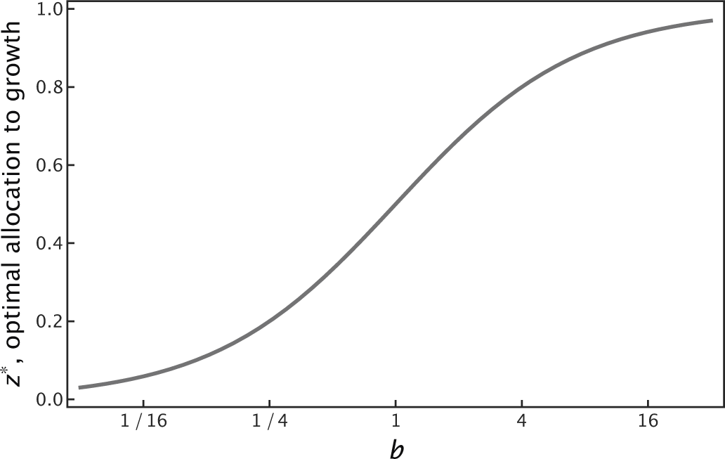
Figure 17.9   Fraction of resources allocated to growth, z^*, with the remaining fraction 1 − z* allocated to storage and survival. Based on the life cycle in Fig. 17.8a, in which individuals pass alternately through growth-favoring and survival-demanding habitats. The optimal allocation depends on b, which determines the marginal gains for growth relative to survival, leading to the solution in eqn 17.13.

Forces acting on traits.—We evaluate forces by studying how changes in traits alter fitness. If we take the demographic context at equilibrium, then we have the fitness expression, W, in eqn 17.10.

As an individual makes small changes in its trait, y, fitness changes by dW/dy evaluated at demographic equilibrium and at trait value equilibrium, y = z = z*, yielding

$$\frac{\mathrm{\text{d}}W}{\mathrm{\text{d}}y}=\left(s^{\prime }{n}^{*}+s^{*}{n}^{\prime }\right)/\lambda +t^{\prime },$$

in which primes denote differentiation with respect to y evaluated at trait value equilibrium. We can find a candidate optimum by setting this expression to zero. Multiplying by λ/s*n* yields

$$\frac{s^{\prime }}{s^{*}}+\frac{n^{\prime }}{n^{*}}+\frac{t^{\prime }}{s^{*}{n}^{*}/\lambda }=0.\text{(17.11)}$$

At the optimum, for each fitness component, any normalized marginal gain with respect to changing trait value is balanced by an equal marginal loss in the other fitness components. These marginal changes follow from the force perturbations caused by trait variations near equilibrium.

Figure 17.10   Optimal growth allocation in relation to p, which determines the fraction of the life cycle spent in survival-demanding (H₂) versus growth-favoring (H₁) conditions. A rise in c increases the relative efficiency of converting resources into growth versus storage. Based on the life cycle in Fig. 17.8b and the solution in eqn 17.14.

Marginal growth benefit.—For the case in Fig. 17.8a, the marginal valuations at the optimum are

$$\frac{n^{\prime }}{n^{*}}=-\frac{s^{\prime }}{s^{*}},$$

which yields

$$\frac{b}{z^{*}}=\frac{1}{1-z^{*}},\text{(17.12)}$$

leading to

$$z^{*}=b/\left(b+1\right)\text{(17.13)}$$

for the optimal fraction of resources allocated to growth in H₁ instead of survival in H₂. The marginal benefit for growth rises with b, favoring more investment in growth, z^*, and less in survival, 1 − z* (Fig. 17.9).

Repeated survival challenge and reproductive value.—The life cycle in Fig. 17.8b splits survivors from the nonreproductive habitat, H₂, into a fraction p that return to the reproductive habitat and a fraction 1 − p that remain in H₂. When remaining in H₂, survival depends on continued use of stored resources.

The extended periods in H₂ raise the valuation of survival relative to growth. Demographic analysis provides a way to study the relative values of alternative fitness components.

Using the general solution in eqn 17.11 and assuming b = 1 to highlight the demographic factors in the life cycle, we obtain the optimum fraction of resources allocated to growth instead of storage and survival as

$$z^{*}=\frac{1-p-\sqrt{cp}}{1-p-2\sqrt{cp}}.\text{(17.14)}$$

Figure 17.10 illustrates the solution. As p declines, individuals increasingly remain in H₂, where they must survive on their stored resources. That greater valuation weighting for survival decreases the optimal fraction of resources allocated to growth.

By contrast, an increase in c enhances the relative efficiency of converting resources to growth versus storage, favoring greater allocation to growth.

Rate versus yield and the genetic structure of populations.—For the life cycle in Fig. 17.8c, growth in habitat H₁ includes competition between different genotypes. Fitness in that habitat follows the basic tragedy of the commons scenario from eqn 5.1. When c = 1 we have

$$w=\frac{y}{z}\left(1-z\right),$$

in which y is a random focal individual’s fractional allocation to growth, and z is the local group of competitors’ average allocation to growth. Using the methods in Section 5.2, the optimal allocation to growth when applied to this fitness component alone would be

z* = 1 − r,

in which r is a generalized notion of a kin selection coefficient as r = dz/dy, the slope group phenotype on the focal individual’s phenotypic value that transmits to future generations. At the optimum, with y = z = z*, fitness is w = r.

The optimum expresses a simple rate versus yield tradeoff. As relatedness, r, increases, the allocation to growth, z^*, declines. With less allocation to growth, the competition between different types for local resources also declines.

Figure 17.11   Mixed-type competition in the growth habitat, H₁, induces a growth rate versus biomass yield tradeoff that alters the growth versus storage allocation. As the parameter r rises, less mixing occurs, favoring greater overall yield efficiency and less allocation to growth. Based on the life cycle in Fig. 17.8c and the solution in eqn 17.15.

Lower short-term growth rate and resource competition increase fitness, effectively raising the yield per unit of available resource.

Alternatively, lower relatedness causes more competition between types, faster short-term growth, and lower efficiency and long-term yield.

In this life cycle, the tragedy of the commons in H₁ embeds within a broader demographic context. For the full demography in Fig. 17.8c, and with c = 1 for simplicity, the optimum is

$$z^{*}=\left(\frac{p}{1+p}\right)\left(1-r\right),\text{(17.15)}$$

with fitness at the optimum of W = 1 + pr, illustrated in Fig. 17.11.

Demographically, lower p values increase the time that individuals spend in the survival-demanding habitat, H₂, favoring greater allocation to storage over growth.

APPLICATIONS TO INDUSTRIAL MICROBIOLOGY

In the wastewater treatment cycle of Fig. 17.6, controlling microbial competition and evolution sets a primary challenge in application. Many applied microbiology problems face similar challenges of managing microbial evolution.

How can we connect the simple abstract models to those real problems and their complex life cycles? That question defines a significant and challenging unsolved research goal.

One often gains the most insight by analyzing the same problem with multiple analytical and conceptual approaches. If attacking this challenge myself, I would consider initially a classical differential equation analysis and an agent-based computer simulation, allowing all potentially interesting assumptions about the biology.

I would then try to parse the complex dynamics into understandable forces. How do those forces dominate as causes of variation in outcome? Can I formulate partial causes that can be expressed as testable comparative hypotheses? Almost always, progress in understanding will depend on simple, clear comparative hypotheses.

It may be possible to improve control by analyzing dynamical models of how populations change. However, such control by dynamical analysis alone is often achieved without a clear understanding of the underlying forces that drive the change. Without that understanding, solutions tend to be fragile. By contrast, understanding the forces allows us to predict how an altered force changes motion.

Industrial microbiology provides great opportunities for the study of microbial design. Progress in understanding the forces of design will improve efficiency in application.

17.4 Challenges in the Study of Design

The simple models we have discussed have strengths and weaknesses.

On the strong side, the models highlight the three fundamental forces of design.122 Marginal values set the tradeoffs between alternative allocations for limited resources. Reproductive values account for how demography weights fitness components, such as growth, survival, and success in different habitats. Generalized kin and similarity selection measure how interactions between different types alter the transmission of traits through time.

These fundamental forces recur in essentially every natural situation. Changes in the environment often influence design by altering these fundamental forces.

For example, biophysical properties such as diffusion of resources or viscosity-limited cellular movement may have several consequences. They can alter the marginal gains obtained in return for resources allocated to different traits, modify the demography of the population, and change the amount of mixing between genetic variants.

On the weak side, these simple models face various difficulties. Optimal traits in equilibrium rarely exist in nature. In any particular situation, many unmodeled environmental parameters alter trait values and population dynamics. The list goes on.

Why have I emphasized simple models, given their certain failure to explain exactly what we see in any application?

Because this book is about isolating component forces and partial causes. Studying how natural processes design organisms is profoundly difficult. We have no chance unless we can break down the complexity into smaller pieces that we can potentially study and understand.

Simple models, with a focus on fundamental forces, provide one tool to study design. Other analyses, such as standard models of differential equations and dynamics, provide different tools.

When building something complex, we require multiple tools. To say that simple models are misleading because they are not sufficient by themselves is like saying that a screwdriver will disrupt making a house because you cannot build a house with just a screwdriver.

In the simple models, I emphasized component forces. Those component forces isolate partial causes. We understand design by building up understanding from partial causes.

To make progress on real systems, we often need a combination of tools. Standard dynamical models and agent-based computer simulations allow description of detailed natural history and biophysics, with a connection to measured parameters. One gets a sense of how things change. The moving body tells the story of evolutionary design.

The simple models analyze the fundamental forces that act implicitly in dynamical models. As Lanczos²²² said, to enhance understanding of causes, it often pays “to focus on the forces, not on the moving body.” The plot revealed.

Ultimately, the deepest understanding comes from combining the alternative perspectives of motion and force into a unified narrative.