Practice Examination 1
SECTION I
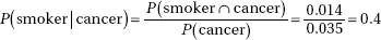
1. (E)
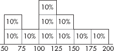
The median price would have 50% of the prices below and 50% of the prices above; however, looking at areas, it is clear that 60% of the prices are below $125,000. The mean (physically the center of gravity) appears to be less than $125,000. Area considerations also show that 30% of the prices are between $100,000 and $125,000. Many values are too far from the mean for the standard deviation to be only $10,000. If the distribution were closer to normal, the standard deviation would be around $25,000; however, the distribution is more spread out than this, and with a SD perhaps between $35,000 and $40,000, estimating the variance at 1.5 × 10⁹ is reasonable.
2. (E) Regression lines show association, not causation. Surveys suggest relationships, which experiments can help to show to be cause and effect.
3. (A) The critical z-score is 1.036. Thus 60 – 55 = 1.036 and = 4.83.
4. (D) We are 90% confident that the population mean is within the interval calculated using the data from the sample.
5. (B) The first study was observational because the subjects were not chosen for treatment.
6. (A)
7. (C) At the dialysis center the more serious concern would be a Type II error, which is that the equipment is not performing correctly, yet the check does not pick this up; while at the towel manufacturing plant the more serious concern would be a Type I error, which is that the equipment is performing correctly, yet the check causes a production halt.
8. (D) There are two possible outcomes (heads and tails), with the probability of heads always 0.75 (independent of what happened on the previous toss), and we are interested in the number of heads in 10 tosses. Thus, this is a binomial model with n = 10 and p = 0.75. Repeating this over and over (in this case 50 times) simulates the resulting binomial distribution.
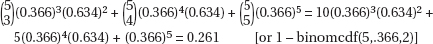
9. (D) In a binomial distribution with probability of success  the probability of at least 3 successes is
+ (0.586)5 = 0.658, or using the TI-83, one finds that 1-binomcdf(5, 0.586, 2) = 0.658.
10. (D) If A and B are mutually exclusive, then P(A  B) = 0, and so P(A ∪ B) = 0.3 + 0.2 – 0 = 0.5. If A and B are independent, then P(A B) = P(A)P(B), and so P(A ∪ B) = 0.3 + 0.2 – (0.3)(0.2) = 0.44. If B is a subset of A, then A ∪ B = A, and so P(A ∪ B) = P(A) = 0.3.
11. (C) The standard deviation of the test statistic is  . Since this is a two-sided test, the P-value will be twice the tail probability of the test statistic; however, the test statistic itself is not doubled.
12. (D) Dosage is the only explanatory variable, and it is being tested at three levels. Tumor reduction is the single response variable.
13. (A) The median corresponds to a cumulative proportion of 0.5.
14. (B) Standard deviation is a measure of variability. The less variability, the more homogeneity.
15. (D) Since the sample sizes are small, the samples must come from normally distributed populations. While the samples should be independent simple random samples, np and n(1 – p) refer to conditions for tests involving sample proportions, not means.
16. (A) Adding the same constant to all values in a set will increase the mean by that constant, but will leave the standard deviation unchanged.
17. (B) With about 68% of the values within 1 standard deviation of the mean, the expected numbers for a normal distribution are as follows:
18. (A) This is a good example of voluntary response bias, which often overrepresents strong or negative opinions. The people who chose to respond were very possibly the parents of children facing drug problems or people who had had bad experiences with drugs being sold in their neighborhoods. There is very little chance that the 2500 respondents were representative of the population. Knowing more about his listeners or taking a sample of the sample would not have helped.
19. (B) The range (difference between largest and smallest values), the interquartile range (Q3 – Q1), and this difference between the 60th and 40th percentile scores all are measures of variability, or how spread out is the population or a subset of the population.
20. (E) Without independence we cannot determine var(X + Y) from the information given.
21. (E) The correlation coefficient r is not affected by changes in units, by which variable is called x or y, or by adding or multiplying all the values of a variable by the same constant.
22. (E) 
23. (B) P(at least one Type I error) = 1 – P(no Type I errors) = 1 – (0.95)10 = 0.40.
24. (E) Note that all three sets have the same mean and the same range. The third set has most of its values concentrated right at the mean, while the second set has most of its values concentrated far from the mean.
25. (C) People coming out of a Wall Street office building are a very unrepresentative sample of the adult population, especially given the question under consideration. Using chance and obtaining a high response rate will not change the selection bias and make this into a well-designed survey. This is a convenience sample, not a voluntary response sample.
26. (C) Larger samples (so  is smaller) and less confidence (so the critical z or t is smaller) both result in smaller intervals.
27. (D) The third scatterplot shows perfect negative association, so r3 = –1. The first scatterplot shows strong, but not perfect, negative correlation, so –1 < r1 < 0. The second scatterplot shows no correlation, so r2 = 0.
28. (D) The probability of throwing heads is 0.5. By the law of large numbers, the more times you flip the coin, the more the relative frequency tends to become closer to this probability. With fewer tosses there is more chance for wide swings in the relative frequency.
29. (C)  If the true mean parking duration is 51 minutes, the normal curve should be centered at 51. The critical value of 50 has a z-score of
30. (A) The overall lengths (between tips of whiskers) are the same, and so the ranges are the same. Just because the min and max are equidistant from the median, and Q1 and Q3 are equidistant from the median, does not imply that a distribution is symmetric or that the mean and median are equal. And even if a distribution is symmetric, this does not imply that it is roughly normal. Particular values, not distributions, may be outliers.
31. (C) Critical z-scores are 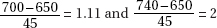 with right tail probabilities of 0.1335 and 0.0228, respectively. The percentage below 740 given that the scores are above 700 is
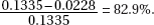
32. (D) There is a different probability of Type II error for each possible correct value of the population parameter, and 1 minus this probability is the power of the test against the associated correct value.
33. (E) This is not a simple random sample because all possible sets of the required size do not have the same chance of being picked. For example, a set of principals all from just half the school districts has no chance of being picked to be the sample. This is not a cluster sample in that there is no reason to believe that each school district resembles the population as a whole, and furthermore, there was no random sample taken of the school districts. This is not systematic sampling as the districts were not put in some order with every nth district chosen. Stratified samples are often easier and less costly to obtain and also make comparative data available. In this case responses can be compared among various districts.
34. (A) A simple random sample can be any size and may or may not be representative of the population. It is a method of selection in which every possible sample of the desired size has an equal chance of being selected.
35. (C) The critical z-scores go from ±1.645 to ±2.576, resulting in an increase in the interval size:  or an increase of 57%.
36. (E) If the P-value is less than 0.10, it does not follow that it is less than 0.05. Decisions such as whether a test should be one- or two-sided are made before the data are gathered. If α = 0.01, there is a 1% chance of rejecting the null hypothesis if the null hypothesis is true. There is one probability of a Type I error, the significance level, while there is a different probability of a Type II error associated with each possible correct alternative, so the sum does not equal 1.
37. (C)  has a t-distribution with df = n – 1.
38. (C) A correlation of 0.6 explains (0.6)2 or 36% of the variation in y, while a correlation of 0.3 explains only (0.3)2 or 9% of the variation in y.
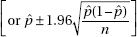
39. (A) Using a measurement from a sample, we are never able to say exactly what a population proportion is; rather we always say we have a certain confidence that the population proportion lies in a particular interval. In this case that interval is 43% ± 5% or between 38% and 48%.
40. (B) With Plan I the expected number of students with stock investments is only 2.4 out of 30. Plan II allows an estimate to be made using a full 30 investors.
SECTION II
1. A complete answer compares shape, center, and spread.
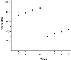
Shape: The baseball players, (A), for which the cumulative frequency plot rises steeply at first, include more shorter players, and thus the distribution is skewed to the right (toward the greater heights). The football players, (C), for which the cumulative frequency plot rises slowly at first, and then steeply toward the end, include more taller players, and thus the distribution is skewed to the left (toward the lower heights). The basketball players, (B), for which the cumulative frequency plot rises slowly at each end, and steeply in the middle, have a more bell-shaped distribution of heights.
Center: The medians correspond to relative frequencies of 0.5. Reading across from 0.5 and then down to the x-axis shows the median heights to be about 63.5 inches for baseball players, about 72.5 inches for basketball players, and about 79 inches for football players. Thus, the center of the baseball height distribution is the least, and the center of the football height distribution is the greatest.
Spread: The range of the football players is the smallest, 80 – 65 = 15 inches, then comes the range of the baseball players, 80 – 60 = 20 inches, and finally the range of the basketball players is the greatest, 85 – 60 = 25 inches.
SCORING
The discussion of shape is essentially correct for correctly identifying which distribution is skewed left, skewed right, and more bell-shaped, and for giving a correct justification based on the cumulative frequency plots. The discussion of shape is partially correct for correctly identifying which distribution is skewed left, skewed right, and more bellshaped without giving a good explanation.
The discussion of center is essentially correct for correctly noting that the baseball players have the lowest median height and the football players have the greatest median height, and giving some numerical justification. The discussion of center is partially correct for correctly noting that the baseball players have the lowest median height and the football players have the greatest median height but without giving a good explanation.
The discussion of spread is essentially correct for correctly noting that the football players have the smallest range for their heights and the basketball players have the greatest range for their heights, and giving some numerical justification. The discussion of spread is partially correct for correctly noting that the football players have the smallest range for their heights and the basketball players have the greatest range for their heights but without giving a good explanation.
4 Complete Answer |
All three parts essentially correct. |
3 Substantial Answer |
Two parts essentially correct and one part partially correct. |
2 Developing Answer |
Two parts essentially correct OR one part essentially correct and one or two parts partially correct OR all three parts partially correct. |
1 Minimal Answer |
One part essentially correct OR two parts partially correct. |
2. (a) A control group would allow the school system to compare the effectiveness of each of the new programs to the local standard method currently being used.
(b) Parents who fail to return the consent form are a special category who may well place less priority on education. The effect of using their children may distort results, since their children could only be placed in the control group.
(c) Assign each student a unique number 01–90. Using a random number table or a random number generator on a calculator, pick numbers between 01 and 90, throwing out repeats. The students corresponding to the first 30 such numbers picked will be assigned to Program A, the next 30 picked to Program B, and the remaining to the control group.
SCORING
Part (a) is essentially correct if the purpose is given for using a control group in this study. Part (a) is partially correct if a correct explanation for the use of a control group is given, but not in context of this study.
Part (b) is essentially correct for a clear explanation in context. Part (b) is partially correct if the explanation is weak.
Part (c) is essentially correct if randomization is used correctly and the method is clear. Part (c) is partially correct if randomization is used but the method is not clearly explained.
4 Complete Answer |
All three parts essentially correct. |
3 Substantial Answer |
Two parts essentially correct and one part partially correct. |
2 Developing Answer |
Two parts essentially correct OR one part essentially correct and one or two parts partially correct OR all three parts partially correct. |
1 Minimal Answer |
One part essentially correct OR two parts partially correct. |
3. (a) This is a paired data test, not a two-sample test. There are four parts to a complete solution.
Part 1: Must state a correct pair of hypotheses.
H0: µd = 0 and Ha: µd > 0, where µd is the mean daily difference in quantity of gas used (in 100 cu ft) between the house without insulation and the house with insulation.
Part 2: Must name the test and check the conditions.
This is a paired t-test, that is, a single sample hypothesis test on the set of differences.
Conditions: Random sample (given), n = 30 is less than 10% of all possible winter days, and n = 30 is sufficiently large for the CLT to apply.
Part 3: Must find the test statistic t and the P-value.
Calculator software (such as T-Test on the TI-84) gives t = 6.4072 and P = 0.0000.
Part 4: Must state the conclusion in context with linkage to the P-value.
With this small a P-value, 0.0000 < 0.05, there is sufficient evidence to reject H0, that is, there is evidence that the mean daily gas usage in a home without the insulation product is greater than the mean daily gas usage in a home with the insulation product.
(b) In the house without the insulation product an estimate for the average increase in quantity of gas used when the outside temperature goes down 1 degree Fahrenheit is 0.15 hundred cubic feet, while in the house with the insulation product an estimate for the average increase in quantity of gas used when the outside temperature goes down 1 degree Fahrenheit is 0.10 hundred cubic feet. So when the temperature goes down, the increase in gas used is less in the house with the insulation product than in the house without the insulation product.
(c) In the house without the insulation product an estimate for the average quantity of gas used when the outside temperature is 0 degrees Fahrenheit is 10.02 hundred cubic feet, while in the house with the insulation product an estimate for the average quantity of gas used when the outside temperature is 0 degrees Fahrenheit is 7.59 hundred cubic feet. So at an outside temperature of 0 degrees Fahrenheit, the average quantity of gas used is less in the house with the insulation product than in the house without the insulation product.
SCORING
In Part (a), Parts 1–2 are essentially correct for a correct statement of the hypotheses (in terms of population means), together with naming the test and checking the conditions, and partially correct for one of Part 1 or Part 2 completely correct.
Parts 3–4 are essentially correct for a correct calculation of both the test statistic t and the P-value, together with a correct conclusion in context linked to the P-value, and partially correct for one of Part 3 or Part 4 completely correct.
Part (b) is essentially correct for giving the correct values for the slopes, in context of the problem, and making a direct comparison. Part (b) is partially correct for giving the correct slopes but missing the context or the direct comparison.
Part (c) is essentially correct for giving the correct values for the y-intercepts, in context of the problem, and making a direct comparison. Part (c) is partially correct for giving the correct y-intercepts but missing the context or the direct comparison.
Count essentially correct answers as one point and partially correct answers as onehalf point.
4 Complete Answer |
Four points |
3 Substantial Answer |
Three points |
2 Developing Answer |
Two points |
1 Minimal Answer |
One point |
Use a holistic approach to decide a score totaling between two numbers.
4. (a) (i) 
(ii) 
(b) (i) 
(ii) 
(c) (i) 1 – (0.88)5 = 0.4723
(ii) 10(0.82)3(0.18)2 + 5(0.82)4(0.18) + (0.82)5 = 0.9563
(d) (i) 
(ii) 
SCORING
There are two probabilities to calculate in each Part (a)–(d). Each Part is essentially correct for both probabilities correctly calculated and partially correct for one probability correctly calculated. In Parts that use results from previous parts, full credit is given for correctly using the results of the earlier Part, whether that earlier calculation was correct or not. For credit for Part (d), a correct methodology must also be shown.
Count partially correct answers as one-half an essentially correct answer.
4 Complete Answer |
Four essentially correct answers. |
3 Substantial Answer |
Three essentially correct answers. |
2 Developing Answer |
Two essentially correct answers. |
1 Minimal Answer |
One essentially correct answer. |
Use a holistic approach to decide a score totaling between two numbers.
5. (a) Identify the confidence interval and check conditions: two-sample t-interval for µdb – µc, the difference in mean cumulative NO2 exposure for drill and blast workers and concrete workers. We are given that we have independent random samples, 115 and 69 are less than 10% of all “drill and blast” and “concrete” workers, respectively, and we note that the sample sizes are large (ndb = 115  30 and nc = 69 30).
Calculate the confidence interval: with df = min(115–1,69–1) = 68,
Interpretation in context: We are 95% confident that the true difference in the mean cumulative NO2 exposure for drill and blast workers and concrete workers is between –1.367 and –0.033 ppm/yr. [On the TI-84, 2-SampTInt gives (–1.362, –0.0381).]
(b) Zero is not in the above 95% confidence interval, so at the α = 0.05 significance level, there is evidence to reject H0: µdb – µc = 0 in favor of Ha: µdb – µc ≠ 0. That is, there is evidence of a difference in mean cumulative NO2 exposure for drill and blast workers and for concrete workers.
(c) With sample sizes this large, the central limit theorem applies and our analysis is valid.
SCORING
Part (a) has two components. The first component, identifying the confidence interval and checking conditions, is essentially correct for naming the confidence interval procedure, noting independent random samples, and noting the large sample sizes. This component is partially correct for correctly noting two of the three points.
The second component of Part (a) is essentially correct for correct mechanics in calculating the confidence interval and for a correct (based on the shown mechanics) interpretation in context, and is partially correct for one of these two features.
Part (b) is essentially correct for noting that zero is not in the interval so the observed difference is significant and stating this in context of the problem. Part (b) is partially correct for noting that zero is not in the interval so the observed difference is significant, but failing to put this conclusion in context of the problem.
Part (c) is essentially correct for relating the central limit theorem (CLT) to the samples being large. Part (c) is partially correct for referring to the CLT or to the large samples, but not linking the two.
Count partially correct answers as one-half an essentially correct answer.
4 Complete Answer |
Four essentially correct answers. |
3 Substantial Answer |
Three essentially correct answers. |
2 Developing Answer |
Two essentially correct answers. |
1 Minimal Answer |
One essentially correct answer. |
Use a holistic approach to decide a score totaling between two numbers.
6. (a) Identify the confidence interval by name or formula.
95% confidence interval for the population proportion
Check the conditions.
Random sample (given), n = 120 is less than 10% of all one-month-old mice, n = 101 10, and n(1 – ) = 19 10.
Calculate the confidence interval.
Calculator software (such as 1-PropZInt on the TI-84) gives (0.77635, 0.90698).
Interpret the confidence interval in context.
We are 95% confident that between 77.6% and 90.7% of mice will gain more weight with no magnetic field.
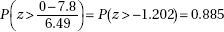
(b) The distribution of the set of all possible differences of weight gains without and with magnetic fields is approximately normal, with mean 25.1 – 17.3 = 7.8 and standard deviation 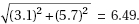 Then the probability that the first mouse gained more weight than the second equals
(c) From the answer to (b), if weight gains without or with the magnetic field are independent, we would expect approximately 88.5% of mice will gain more weight with no magnetic field. From the answer to (a) we estimate the percent of mice who gain more weight with no magnetic field to be between 77.6% and 90.7%. Since 88.5% is in this interval, there is no evidence to suggest that weight gain with no magnetic field and in a magnetic field are not independent.
(d) Calculating 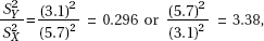 the test statistic is outside the critical cutoff scores of 0.698 and 1.43. Thus there is evidence that the variances of the distributions of weight gains without and with magnetic fields are different.
SCORING
Part (a) has four parts: 1) identifying the confidence interval; 2) checking assumptions; 3) calculating the confidence interval; and 4) interpreting the confidence interval in context. Part (a) is essentially correct if three or four of these parts are correct and partially correct if one or two of these parts are correct.
Part (b) is essentially correct for a complete answer, and partially correct for finding the mean and SD of the set of differences but incorrectly finding the probability, OR making a mistake in finding the mean or standard deviation but using these correctly in finding the probability.
Part (c) is essentially correct for a complete answer and is partially correct if the conclusion is right but the links to (a) and (b) are unclear.
Part (d) is essentially correct for a correct calculation of the quotient of sample variances together with a correct conclusion in context, and is partially correct for one of these two parts correct.
Count partially correct answers as one-half an essentially correct answer.
4 Complete Answer |
Four essentially correct answers. |
3 Substantial Answer |
Three essentially correct answers. |
2 Developing Answer |
Two essentially correct answers. |
1 Minimal Answer |
One essentially correct answer. |
Use a holistic approach to decide a score totaling between two numbers.
Practice Examination 2
SECTION I
1. (D) Since (2, 7) is on the line y = mx + 3, we have 7 = 2m + 3 and m = 2. Thus the regression line is y = 2x + 3. The point (x, y) is always on the regression line, and so we have y = 2x + 3.
2. (B) It could well be that conscientious students are the same ones who both study and do well on the basketball court. If students could be randomly assigned to study or not study, the results would be more meaningful. Of course, ethical considerations might make it impossible to isolate the confounding variable in this way.
3. (B) The critical z-score is 0.525. Thus 75 – µ = 0.525(14) and µ = 67.65.
4. (D) The slope of the regression line and the correlation are related by  When using z-scores, the standard deviations sx and sy are 1. If r = 0, then b1 = 0. Switching which variable is x and which is y, or changing units, will not change the correlation.
5. (E) The median and interquartile range are specifically used when outliers are suspected of unduly influencing the mean, range, or standard deviation.
6. (C) 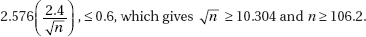
7. (C) This is a hypothesis test with H0: tissue strength is within specifications, and Ha: tissue strength is below specifications. A Type I error is committed when a true null hypothesis is mistakenly rejected.
8. (E) The wording of questions can lead to response bias. The neutral way of asking this question would simply have been, “Do you support the proposed school budget increase?”
9. (D)
10. (E) While it is important to look for basic patterns, it is also important to look for deviations from these patterns. In this case, there is an overall positive correlation; however, those faculty with under ten years of service show little relationship between years of service and salary. While (A) is a true statement, it does not give an overall interpretation of the scatterplot.
11. (D) The second set has a greater range, 3.8 – 1.8 = 2.0 as compared to 4.1 – 2.3 = 1.8, and with its skewness it also has a greater standard deviation.
12. (B) With n = 10, increasing 
13. (B) The means and the variances can be added. Thus the new variance is 52 + 122 = 169, and the new standard deviation is 13.
14. (E) Dice have no memory, so the probability that the next toss will be an even number is 0.5 and the probability that it will be an odd number is 0.5. The law of large numbers says that as the number of tosses becomes larger, the proportion of even numbers tends to become closer to 0.5.
15. (B) The critical t-scores for 90% confidence with df = 7 are ±1.895.
16. (A) Either directly or anonymously, you should be able to obtain the test results for every student.
17. (C) Percentile ranking is a measure of relative position. Adding five points to everyone’s score will not change the relative positions.
18. (A) The control group should have experiences identical to those of the experimental groups except for the treatment under examination. They should not be given a new treatment.
19. (B) If Ha is true, the probability of failing to reject H0 and thus committing a Type II error is 1 minus the power, that is, 1 – 0.8 = 0.2.
20. (C) Five does not split the area in half, so 5 is not the median. Histograms such as these show relative frequencies, not actual frequencies. The area from 1.5 to 4.5 is the same as that between 7.5 and 10.5, each being about 25% of the total. Given the spread, 1 is too small an estimate of the standard deviation. The area above 3 looks to be the same as the area above 9 and 10, so the median won’t change.
21. (D) There must be a fixed number of trials, which rules out (A); only two possible outcomes, which rules out (B); and a constant probability of success on any trial, which rules out (C).
22. (C) In both cases 1 hour is one standard deviation from the mean with a right tail probability of 0.1587.
23. (C) Control, randomization, and replication are all important aspects of well-designed experiments. We try to control lurking variables, not to use them to control something else.
24. (D) The data are strongly skewed to the left, indicating that the mean is less than the median. The median appears to be roughly 215, indicating that the interval [200, 240] probably has more than 50% of the values. While in a standard boxplot each whisker contains 25% of the values, this is a modified boxplot showing four outliers, and so the left whisker has four fewer values than the right whisker.
25. (C) For the regression line, the sum and thus the mean of the residuals are always zero. An influential score may have a small residual but still have a great effect on the regression line. If the correlation is 1, all the residuals would be 0, resulting in a very distinct pattern.
26. (C) 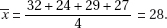 Since (x, y) is a point on the regression line, y = 3(28) + 4 = 88.
27. (C) P(at least 1) = 1 – P(none) = 1 – (0.88)6 = 0.536.
28. (B) Different samples give different sample statistics, all of which are estimates for the same population parameter, and so error, called sampling error, is naturally present.
29. (A) While the associate does use chance, each customer would have the same chance of being selected only if the same number of customers had names starting with each letter of the alphabet. This selection does not result in a simple random sample because each possible set of 104 customers does not have the same chance of being picked as part of the sample. For example, a group of customers whose names all start with A will not be chosen. Sampling error, the natural variation inherent in a survey, is always present and is not a source of bias. Letting the surveyor have free choice in selecting the sample, rather than incorporating chance in the selection process, is a recipe for disaster!
30. (A) Corresponding to cumulative proportions of 0.25 and 0.75 are Q1 = 2.25 and Q3 = 3.1, respectively, and so the interquartile range is 3.1 – 2.25 = 0.85.
31. (E) The standard deviation of the test statistic is 
32. (D) From a table or a calculator (for example invNorm on the TI-84), the 40th percentile corresponds to a z-score of –0.2533, and –0.2533(0.28) = –0.0709.
33. (D) Increasing the sample size by a multiple of d divides the interval estimate by  .
.
34. (D) The t-distributions are symmetric; however, they are lower at the mean and higher at the tails and so are more spread out than the normal distribution. The greater the df, the closer the t-distributions are to the normal distribution. The 68–95–99.7 Rule applies to the z-distribution and will work for t-models with very large df. All probability density curves have an area of 1 below them.
35. (E) The given bar chart shows percentages, not actual numbers.
36. (C) This follows from the central limit theorem.
37. (E) There is a different Type II error for each possible correct value for the population parameter.
38. (C) X is close to the mean and so will have a z-score close to 0. Modified boxplots show only outliers that are far from the mean. X and the two clusters are clearly visible in a stemplot of these data. In symmetric distributions the mean and median are equal. The IQR here is close to the range.
39. (E) Using a measurement from a sample, we are never able to say exactly what a population proportion is; rather we always say we have a certain confidence that the population proportion lies in a particular interval. In this case that interval is 82% ± 3% or between 79% and 85%.
40. (A) Whether or not students are taking AP Statistics seems to have no relationship to which type of school they are planning to go to. Chi-square is close to 0.
SECTION II
Part A
1. (a) Number the volunteers 1 through 10. Use a random number generator to pick numbers between 1 and 10, throwing out repeats. The volunteers corresponding to the first two numbers chosen will receive aloe, the next two will receive camphor, the next two eucalyptus oil, the next two benzocaine, and the remaining two a placebo.
(b) Each volunteer (the volunteers are “blocks”) should receive all five treatments, one a day, with the time-order randomized. For example, label aloe 1, camphor 2, eucalyptus oil 3, benzocaine 4, and the placebo 5. Then for each volunteer use a random number generator to pick numbers between 1 and 5, throwing away repeats. The order picked gives the day on which each volunteer receives each treatment.
(c) Results cannot be generalized to women.
SCORING
Part (a) is essentially correct for giving a procedure which randomly assigns 2 volunteers to each of the five treatments. Part (a) is partially correct for giving a procedure which randomly assigns one of the treatments for each volunteer, but may not result in two volunteers receiving each treatment.
Part (b) is essentially correct for giving a procedure which assigns a random order for each of the volunteers to have all 5 treatments. Part (b) is partially correct for having each volunteer take all five treatments, one a day, but not clearly randomizing the time-order.
Part (c) is essentially correct for stating that the results cannot be generalized to women and is incorrect otherwise.
4 Complete Answer |
All three parts essentially correct. |
3 Substantial Answer |
Two parts essentially correct and one part partially correct. |
2 Developing Answer |
Two parts essentially correct OR one part essentially correct and one or two parts partially correct OR all three parts partially correct. |
1 Minimal Answer |
One part essentially correct OR two parts partially correct. |
2. (a)  =
=  xp(x) = 0(0.05) + 1(0.10) + 2(0.13) + 3(0.15) + 4(0.14) + 5(0.12) + 6(0.10) + 7(0.08) + 8(0.06) + 9(0.04) + 10(0.03) = 4.27.
With (0.05 + 0.10 + 0.13 + 0.15) = 0.43 below 4 runs, and (0.12 + 0.10 + 0.08 + 0.06 + 0.04 + 0.03) = 0.43 above 4 runs, the median must be 4.
(b) The mean is greater than the median, as was to be expected because the distribution is skewed to the right.
(c) P(at least one shutout in 4 games) = 1 – P(no shutouts in the 4 games)
= 1 – (1 – 0.05)4 = 1 – (0.95)4 = 0.1855
(d) The distribution of x is approximately normal with mean µx = 4.27 (from above) and standard deviation 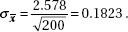
SCORING
Part (a) is essentially correct for correctly calculating both the mean and median. Part (a) is partially correct for correctly calculating one of these two measures.
Part (b) is essentially correct for noting that the mean is greater than the median and relating this to the skew.
Part (c) is essentially correct for recognizing this as a binomial probability calculation and making the correct calculation. Part (c) is partially correct for recognizing this as a binomial probability calculation, but with an error such as 1 – (0.05)4 or 4(0.05)(0.95)3.
Part (d) is essentially correct for “approximately normal,” µx = 4.27, and x = 0.1823, and partially correct for two of these three answers.
Count partially correct answers as one-half an essentially correct answer.
4 Complete Answer |
Four essentially correct answers. |
3 Substantial Answer |
Three essentially correct answers. |
2 Developing Answer |
Two essentially correct answers. |
1 Minimal Answer |
One essentially correct answer. |
Use a holistic approach to decide a score totaling between two numbers.
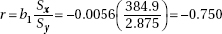
3. (a) The slope b1 is in the center of the confidence interval, so  –0.0056. In context, 0.0056 estimates the average decrease in the manic-depressive scale score for each 1-microgram increase in the level of urinary MHPG. (Thus high levels of MHPG are associated with increased mania, and conversely, low levels of MHPG are associated with increased depression.)
(b) Recalling that the regression line goes through the point (x, y) or using the AP Exam formula page, bo = y – b1x = 5.4 – (–0.0056)(1243.1) = 12.36, and thus the equation of the regression line is  = 12.36 – 0.0056(MHPG) (or
  = 12.36 – 0.0056x, where x is the level of urinary MHPG in micrograms per 24 hours, and y is the score on a 0–10 manic-depressive scale).
(c) Recalling that on the regression line, each one SD increase in the independent variable corresponds to an increase of r SD in the dependent variable, or using the AP
Exam formula page, 
and r2 = 56.2%. Thus, 56.2% of the variation in the manic-depression scale level is explained by urinary MHPG levels.
(d) Correlation never proves causation. It could be that depression causes biochemical changes leading to low levels of urinary MHPG, or it could be that low levels of urinary MHPG cause depression, or it could be that some other variable (a lurking variable) simultaneously affects both urinary MHPG levels and depression.
SCORING
Part (a) is essentially correct if the slope is correctly calculated and correctly interpreted in context. Part (a) is partially correct if the slope is not correctly calculated but a correct interpretation is given using the incorrect value for the slope.
Part (b) is essentially correct if the regression equation is correctly calculated (using the slope found in part (a)) and it is clear what the variables stand for. Part (b) is partially correct if the correct equation is found (using the slope found in part (a)) but it is unclear what the variables stand for.
Part (c) is essentially correct if the coefficient of determination, r2, is correctly calculated and correctly interpreted in context. Part (c) is partially correct if r2 is not correctly calculated but a correct interpretation is given using the incorrect value for r2.
Part (d) is essentially correct for noting that correlation never proves causation, and referring to context. Part (d) is partially correct for a correct statement about correlation and causation, but with no reference to context.
Count partially correct answers as one-half an essentially correct answer.
4 Complete Answer |
Four essentially correct answers. |
3 Substantial Answer |
Three essentially correct answers. |
2 Developing Answer |
Two essentially correct answers. |
1 Minimal Answer |
One essentially correct answer. |
Use a holistic approach to decide a score totaling between two numbers.
4. There are four parts to this solution.
(a) State the hypotheses.
H0: µ1 – µ2 = 0 and Ha: µ1 – µ2 < 0
where µ1 = mean number of months at which first steps alone are taken for infants receiving daily stimulation, and µ2 = mean number of months at which first steps are taken for infants in the control group. [Other notations are also possible, for example, H0: µ1 = µ2 and Ha: µ1 < µ2.]
(b) Identify the test by name or formula and check the assumptions.
Two-sample t-test OR 
Conditions: We are given that the infants were randomly assigned to the two groups, n = 20 is less than 10% of all infants, and dotplots of the two groups show no outliers and are roughly bell-shaped.
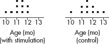
(c) Mechanics: Putting the data into two Lists, calculator software (such as 2-SampTTest on the TI-84) gives t = –1.2 and P = 0.12345.
(d) State the conclusion in context with linkage to the P-value.
With this large a P-value, 0.12345 > 0.05, there is not sufficient evidence to reject H0, that is, there is not sufficient evidence that infants walk earlier with daily stimulation of specific reflexes.
SCORING
Part (a) is essentially correct for stating the hypotheses and identifying the variables. Part (a) is partially correct for correct hypotheses, but missing identification of the variables.
Part (b) is essentially correct for identifying the test and checking the assumptions. Part (b) is partially correct for only one of these two elements.
Part (c) is essentially correct for correctly calculating both the t-score and the P-value. Part (c) is partially correct for only one of these two elements.
Part (d) is essentially correct for a conclusion in context with linkage to the P-value. Part (d) is partially correct for only one of these two elements.
Count partially correct answers as one-half an essentially correct answer.
4 Complete Answer |
Four essentially correct answers. |
3 Substantial Answer |
Three essentially correct answers. |
2 Developing Answer |
Two essentially correct answers. |
1 Minimal Answer |
One essentially correct answer. |
Use a holistic approach to decide a score totaling between two numbers.
5. (a) A complete answer compares shape, center, and spread.
Shape: The 10-kilometer distribution appears symmetric, while the 5-mile distribution is skewed right.
Center: The median of the 10-kilometer distribution is 4 minutes greater than the median of the 5-mile distribution.
Spread: The ranges of the two distributions are equal, both about 7 minutes.
(b) Shape: Again, the 10-kilometer distribution appears symmetric, while the 5-mile distribution is still skewed right.
Center: Now the median of the 10-kilometer distribution is about 3.5 minutes less than the median of the 5-mile distribution.
Spread: Now the range of the 10-kilometer distribution is less than the range of the 5-mile distribution.
(c) One possible answer is that this was not as expected with the following explanation: One would expect that for 5 miles, the shorter run, the speeds would be faster, so adjusting the 5-mile run times would result in faster times (less minutes) than the 10-kilometer times, but this was not the case. [Perhaps slower, less serious runners participate in the shorter race, so when their times are adjusted, the minutes are greater than the times for the 10-kilometer run.]
(d) In each set of parallel boxplots, the 10-kilometer distribution appears symmetric, so that the mean will be about the same as the median, while the 5-mile distribution is skewed right so that the mean will in all likelihood be greater than the median. In the first set of boxplots (where the 5-mile median < 10-kilometer median) this will result in the means being closer, while in the second set of boxplots (where the 5-mile median > 10-kilometer median) this will result in the means being further apart. Thus we would expect the difference in mean times in the first set of parallel boxplots to be less than the difference in mean times in the second set of parallel boxplots.
SCORING
Part (a) is essentially correct for correctly comparing shape, center, and spread. Part (a) is partially correct for correctly comparing two of the three features.
Part (b) is essentially correct for correctly comparing shape, center, and spread. Part (b) is partially correct for correctly comparing two of the three features.
Part (c) is essentially correct for a reasonable statement about the change between the two sets of parallel boxplots together with a correct explanation to go along with the statement. Part (c) is partially correct if the explanation is weak.
Part (d) is essentially correct for a correct prediction about the means together with a reasonable justification based on symmetry of the 10-kilometer distribution and skewness of the 5-mile distribution. Part (d) is partially correct if the justification is weak.
Count partially correct answers as one-half an essentially correct answer.
4 Complete Answer |
Four essentially correct answers. |
3 Substantial Answer |
Three essentially correct answers. |
2 Developing Answer |
Two essentially correct answers. |
1 Minimal Answer |
One essentially correct answer. |
Use a holistic approach to decide a score totaling between two numbers.
SECTION II
Part B
6. (a) Identify the confidence interval by name or formula.
z-interval of a population proportion or 
Conditions: Random sample (given), n = 250 is less than 10% of all SAT math scores, n = 82 + 36 + 12 = 130 10, and n(1 – ) = 250 –130 = 120 10.
Mechanics: Calculator software (such as 1-PropZInt on the TI-84) gives (0.45807, 0.58193).
Interpret the confidence interval in context.
We are 95% confident that between 45.8% and 58.2% of SAT mathematics scores are over 500.
(b) State the hypotheses.
H0: The distribution of SAT mathematics scores is normal with µ = 500 and = 100.
Ha: The distribution of SAT mathematics scores is not normal with µ = 500 and = 100.
Identify the test by name or formula and check the assumptions.
Chi-square goodness-of-fit test
Check conditions
We have a random sample.
A normal distribution has 34.13% on each side of the mean and within one SD, 13.59% on each side between one and two SDs from the mean, and 2.28% on each side more than two SDs from the mean. This gives expected cell counts of (0.0228)250 = 5.7, (0.1359)500 = 34.0, and (0.3413)500 = 85.3, each of which is at least 5.
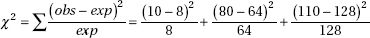
Mechanics: Put {7, 39, 74, 82, 36, 12} in one List and {5.7, 34.0, 85.3, 85.3, 34.0, 5.7} in a second List. With df = 6 – 1 = 5, calculator software (such as χ2GOF-Test on the TI-84) gives χ2 = 9.7372 and P = 0.0830.
State the conclusion in context with linkage to the P-value.
With this large a P-value, 0.0830 > 0.05, there is not sufficient evidence to reject H0, that is, there is not sufficient evidence that the distribution of SAT math scores is not normal.
(c)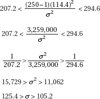
Thus we are 95% confident that the standard deviation for the distribution of SAT mathematics scores is between 105.2 and 125.4.
SCORING
Part (a) has four parts: 1) identifying the confidence interval; 2) checking assumptions; 3) calculating the confidence interval; and 4) interpreting the confidence interval in context. Part (a) is essentially correct if three or four of these parts are correct and partially correct if one or two of these parts are correct.
Part (b) has four parts: 1) stating the hypotheses; 2) identifying the test and checking assumptions; 3) calculating the test statistic and the P-value; and 4) giving a conclusion in context with linkage to the P-value. Part (b) is essentially correct if three or four of these parts are correct and partially correct if one or two of these parts are correct.
Part (c) is essentially correct for calculating the confidence interval and interpreting it in context. Part (c) is partially correct for one of these two parts correct.
4 Complete Answer |
All three parts essentially correct. |
3 Substantial Answer |
Two parts essentially correct and one part partially correct. |
2 Developing Answer |
Two parts essentially correct OR one part essentially correct and one or two parts partially correct OR all three parts partially correct. |
1 Minimal Answer |
One part essentially correct OR two parts partially correct. |
Practice Examination 3
SECTION I
1. (C) A complete census can give much information about a population, but it doesn’t necessarily establish a cause-and-effect relationship among seemingly related population parameters. While the results of well-designed observational studies might suggest relationships, it is difficult to conclude that there is cause and effect without running a well-designed experiment. If bias is present, increasing the sample size simply magnifies the bias. The control group is selected by the researchers making use of chance procedures.
2. (A) In the first class only 40% of the students scored below the given score, while in the second class 80% scored below the same score.
3. (C) The control group should have experiences identical to those of the experimental groups except for the treatment under examination. They should not be given a new treatment.
4. (E) The negative sign comes about because we are dealing with the difference of proportions. The confidence interval estimate means that we have a certain confidence that the difference in population proportions lies in a particular interval.
5. (B) The desire of the workers for the study to be successful led to a placebo effect.
6. (E) The proportion of successful calls (problem solved) is  is the expected number of calls from location 1 that are successful. Alternatively, the proportion of calls from location 1 is so
  gives the expected number of successful calls from location 1.
7. (C) The slope and the correlation always have the same sign. Correlation shows association, not causation. Correlation does not apply to categorical data. Correlation measures linear association, so even with a correlation of 0, there may be very strong nonlinear association.
8. (B) If two random variables are independent, the mean of the difference of the two random variables is equal to the difference of the two individual means; however, the variance of the difference of the two random variables is equal to the sum of the two individual variances.
9. (D) A sample is simply a subset of a population.
10. (B) The markings, spaced 15 apart, clearly look like the standard deviation spacings associated with a normal curve.
11. (B) With a right tail having probability 0.01, the critical z-score is 2.326. Thus µ + 2.326(0.3) = 12, giving µ = 11.3.
12. (E) There is no reason to think that AAA members are representative of the city’s drivers. Family members may have similar driving habits and the independence condition would be violated. Random selection is important regardless of the sample size. The larger a random sample, the closer its standard deviation will be to the population standard deviation.
13. (D)
14. (C) As n increases the probabilities of Type I and Type II errors both decrease.
15. (A) The mean equals the common value of all the data elements. The other terms all measure variability, which is zero when all the data elements are equal.
16. (E)  and with df = 15 – 1 = 14, the critical t-scores are ±1.761.
17. (E) In a simple random sample, every possible group of the given size has to be equally likely to be selected, and this is not true here. For example, with this procedure it is impossible for the employees in the final sample to all be from a single plant. This method is an example of stratified sampling, but stratified sampling does not result in simple random samples.
18. (D) (0.32)(0.15) = 0.048 so P(E F) = P(E)P(F) and thus E and F are independent. P(E F) ≠ 0, so E and F are not mutually exclusive.
19. (A) The quartiles Q1 and Q3 have z-scores of ±0.67, so Q1 = 640,000 – (0.67)18,000 ≈ 628,000, while Q3 = 640,000 + (0.67)18,000 ≈ 652,000. The interquartile range is the difference Q3 – Q1.
20. (D) One set is a shift of 20 units from the other, so they have different means and medians, but they have identical shapes and thus the same variability including IQR, standard deviation, and variance.
21. (B) A 99% confidence interval estimate means that in about 99% of all samples selected by this method, the population mean will be included in the confidence interval. The wider the confidence interval, the higher the confidence level. The central limit theorem applies to any population, no matter if it is normally distributed or not. The sampling distribution for a mean always has standard deviation  large enough sample size n refers to the closer the distribution will be to a normal distribution. The center of a confidence interval is the sample statistic, not the population parameter.
22. (E) In none of these are the trials independent. For example, as each consecutive person is stopped at a roadblock, the probability the next person has a seat belt on will quickly increase; if a student has one A, the probability is increased that he or she has another A.
23. (E) Independence implies P(E F) = P(E)P(F), while mutually exclusive implies P(E F) = 0.
24. (E) In a binomial with n = 4 and p = 0.9, P(at least 3 successes) = P(exactly 3 successes) + P(exactly 4 successes) = 4(0.9)3(0.1) + (0.9)4.
25. (C) In stratified sampling the population is divided into representative groups, and random samples of persons from each group are chosen. In this case it might well be important to be able to consider separately the responses from each of the three groups—urban, suburban, and rural.
26. (E) r2, the coefficient of determination, indicates the percentage of variation in y that is explained by variation in x.
27. (C) It is most likely that the homes at which the interviewer had difficulty finding someone home were homes with fewer children living in them. Replacing these homes with other randomly picked homes will most likely replace homes with fewer children with homes with more children.
28. (A) The median corresponds to the 0.5 cumulative proportion.
29. (A) Blocking divides the subjects into groups of similar individuals, in this case individuals with similar exercise habits, and runs the experiment on each separate group. This controls the known effect of variation in exercise level on cholesterol level.
30. (B) The margin of error varies directly with the critical z-value and directly with the standard deviation of the sample, but inversely with the square root of the sample size.
31. (E)  With a true mean increase of 4.2, the z-score for 4.0 is
  –1.25 and the officers fail to reject the claim if the sample mean has z-score greater than this.
32. (E) Both have 50 for their means and medians, both have a range of 90 – 10 = 80, and both have identical boxplots, with first quartile 30 and third quartile 70.
33. (B) Since we are not told that the investigator suspects that the average weight is over 300 mg or is under 300 mg, and since a tablet containing too little or too much of a drug clearly should be brought to the manufacturer’s attention, this is a two-sided test. Thus the P-value is twice the tail probability obtained (using the t-distribution with df = n – 1 = 6).
34. (A) This study was an experiment because a treatment (weekly quizzes) was imposed on the subjects. However, it was a poorly designed experiment with no use of randomization and no control over lurking variables.
35. (C) The expected frequencies, as calculated by the rule in (E), may not be whole numbers.
36. (E) The probabilities of Type I and Type II error are related; for example, lowering the Type I error increases the probability of a Type II error. A Type I error can be made only if the null hypothesis is true, while a Type II error can be made only if the null hypothesis is false. In medical testing, with the usual null hypothesis that the patient is healthy, a Type I error is that a healthy patient is diagnosed with a disease, that is, a false positive. We reject H0 when the P-value falls below α, and when H0 is true this rejection will happen precisely with probability α.
37. (C) X is probably very close to the least squares regression line and so has a small residual. Removing X will change the regression line very little if at all, and so it is not an influential point. The association between the x and y variables is very strong, just not linear. Correlation measures the strength of a linear relationship, which is very weak regardless of whether the point X is present or not.
38. (B) The probability of an application being turned down is 1 – 0.90 = 0.10, and the expected value of a binomial with n = 50 and p = 0.10 is np = 50(0.10).
39. (E) A boxplot gives a five-number summary: smallest value, 25th percentile (Q1), median, 75th percentile (Q3), and largest value. The interquartile range is given by Q3 – Q1, or the total length of the two “boxes” minus the “whiskers.”
40. (E) Using a measurement from a sample, we are never able to say exactly what a population mean is; rather we always say we have a certain confidence that the population mean lies in a particular interval.
SECTION II
Part A
1. (a) A complete answer compares shape, center, and spread.
Shape. The control group distribution is somewhat bell-shaped and symmetric, while the treatment group distribution is somewhat skewed right.
Center. The center of the control group distribution is around 20, which is greater than the center of the treatment group distribution, which is somewhere around 10 to 12.
Spread. The spread of the control group distribution, 5 to 34, is less than the spread of the treatment group distribution, which is 2 to 41.
(b) For computers in the control group (no spam software), the number of spam e-mails received varies an “average” amount of 8.1 from the mean number of spam e-mails received in the control group.
(c) Since the 95% confidence interval for the difference does not contain zero, the researcher can conclude the observed difference in mean numbers of spam e-mails received between the control group and the treatment group that received spam software is significant.
(d) It may well be that the four groups—administrators, staff, faculty, and students—are each exposed to different kinds of spam e-mail risks, and possibly the software will be more or less of a help to each group. In that case, the researcher should in effect run four separate experiments on the homogeneous groups, called blocks. Conclusions will be more specific.
SCORING
Part (a) is essentially correct for correctly comparing shape, center, and spread. Part (a) is partially correct for correctly comparing two of the three features.
Part (b) is essentially correct if standard deviation is explained correctly in context of this problem. Part (b) is partially correct if there is a correct explanation of SD but no reference to context.
Part (c) is essentially correct for noting that zero is not in the interval so the observed difference is significant, and stating this in context of the problem. Part (c) is partially correct for noting that zero is not in the interval so the observed difference is significant, but failing to put this conclusion in context of the problem.
Part (d) is essentially correct if the purpose of blocking is correctly explained in context of this problem. Part (d) is partially correct if the general purpose of blocking is correctly explained but not in context of this problem.
Count partially correct answers as one-half an essentially correct answer.
4 Complete Answer |
Four essentially correct answers. |
3 Substantial Answer |
Three essentially correct answers. |
2 Developing Answer |
Two essentially correct answers. |
1 Minimal Answer |
One essentially correct answer. |
Use a holistic approach to decide a score totaling between two numbers.
2. (a) Listing the eight possibilities: {HHH, HHT, HTH, HTT, THH, THT, TTH, TTT} clearly shows that the only possibilities for the absolute value of the difference are 1 with probability 6/8 = 0.75 and 3 with probability 2/8 = 0.25. The table is:
(b) E = xP(x) = 1(0.75) + 3(0.25) = 1.5
(c) Since the only possible scores for each game are 1 and 3, the only way to have a total score of 3 in three games is to score 1 in each game. The probability of this is 
(d) The more times the game is played, the closer the average score will be to the expected value of 1.5. The player does not want to average close to 1.5, so should prefer playing 10 times rather than 15 times.
SCORING
Part (a) is essentially correct for the correct probability distribution table. Part (a) is partially correct for one minor error.
Part (b) is essentially correct for the correct calculation of expected value based on the answer given in Part (a). Part (b) is partially correct for the correct formula for expected value but an incorrect calculation based on the answer given in Part (a).
Part (c) is essentially correct for the correct probability calculation with some indication of where the answer is coming from. Part (c) is partially correct for the correct probability with no work shown.
Part (d) is essentially correct for choosing 10 and giving a clear explanation. Part (d) is partially correct for choosing 10 and giving a weak explanation. Part (d) is incorrect for choosing 10 with no explanation or with an incorrect explanation.
Count partially correct answers as one-half an essentially correct answer.
4 Complete Answer |
Four essentially correct answers. |
3 Substantial Answer |
Three essentially correct answers. |
2 Developing Answer |
Two essentially correct answers. |
1 Minimal Answer |
One essentially correct answer. |
Use a holistic approach to decide a score totaling between two numbers.
3. (a) The slope of –7.19 says that the attendance dropped an average of 7.19 students per week. No, this does not seem to adequately explain the data, because the attendance increased every week during the first 4 weeks, and again increased every week during the final 4 weeks.
(b) Modeling the first 4 weeks (computer games allowed) gives  5.1(Week) with r = 0.997, and modeling the final 4 weeks (no computer games) gives
  (Week) with r = 0.997. These models give an average increase in attendance each week of 5.1 and 4.9, respectively, as well as much higher correlations.
(c)
The scatterplot clearly shows the linearity in the first 4 weeks and in the final 4 weeks, and also the nonlinearity of the full set of data.
SCORING
Part (a) is essentially correct if the slope is correctly interpreted in context and a reasonable explanation is given as to why this slope does not explain the data. Part (a) is partially correct if one of these two components is correct.
Part (b) is essentially correct for two separate regression models, correct interpretations of the slopes, and noting the increased correlation. Part (b) is partially correct if one of these components is missing.
Part (c) is essentially correct if the scatterplot is correctly drawn and the strong linearity in the first four weeks and separately in the final four weeks is noted. Part (c) is partially correct for a correctly drawn scatterplot but no observations on linearity.
4 Complete Answer |
All three parts essentially correct. |
3 Substantial Answer |
Two parts essentially correct and one part partially correct. |
2 Developing Answer |
Two parts essentially correct OR one part essentially correct and one or two parts partially correct OR all three parts partially correct. |
1 Minimal Answer |
One part essentially correct OR two parts partially correct. |
4. This is a paired data test, not a two-sample test, with four parts to a complete solution.
Part 1: Must state a correct pair of hypotheses.
Either H0 : µd = 0 and Ha : µd < 0 where µd is the mean difference between the investigator and facility estimates; or
H0 : µ1 – µ2 = 0 and Ha : µ1 – µ2 < 0 where µ1 is the mean estimate of the investigator and µ2 is the mean estimate of the facility.
Part 2: Must name the test and check the conditions.
This is a paired t-test, that is, a single sample hypothesis test on the set of differences.
Conditions:
Random sample (given) and it is reasonable to assume that the 10 data pairs are independent of each other. Normality of the population distribution of differences should be checked graphically on the sample data using a histogram, or a boxplot, or a normal probability plot:
Part 3: Must find the test statistic t and the P-value.
Putting the differences {335, –560, …, –380} in a List, calculator software (such as T-Test on the TI-84) gives t = –2.564 and P = 0.0152.
Part 4: Linking to the P-value, give a correct conclusion in context.
With this small a P-value, 0.0152 < 0.05, there is evidence to reject H0. That is, there is evidence that the mean estimate of the facility under suspicion is greater than the mean estimate by the investigators.
SCORING
Part 1 is essentially correct for a correct statement of the hypotheses (in terms of population means).
Part 2 is essentially correct if the test is correctly identified by name or formula and a graphical check of the normality condition is given.
Part 3 is essentially correct for a correct calculation of both the test statistic t and the P-value.
Part 4 is essentially correct for a correct conclusion in context, linked to the P-value.
4 Complete Answer |
All four essentially correct answers. |
3 Substantial Answer |
Three essentially correct answers. |
2 Developing Answer |
Two essentially correct answers. |
1 Minimal Answer |
One essentially correct answer. |
5. (a) A statistic used to estimate a population parameter is unbiased if the mean of the sampling distribution of the statistic is equal to the true value of the parameter being estimated. Estimators B, C, and D appear to have means equal to the population mean of 146.
(b) For n = 40, estimator A exhibits the lowest variability, with a range of only 2 grams compared to the other ranges of 6 grams, 4 grams, 4 grams, and 4 grams.
(c) The estimator should have a distribution centered at 146, thus eliminating A and E. As n increases, D shows tighter clustering around 146 than does B. Finally, while C looks better than D for n = 40, the estimator will be used with n = 100, and the D distribution is clearly converging as the sample size increases while the C distribution remains the same. Choose D.
SCORING
Part (a) is essentially correct for a correct answer with a good explanation of what unbiased means, and is partially correct for a correct answer with a weak explanation. Part (a) is incorrect for a correct answer with no explanation or with an incorrect explanation.
Part (b) is essentially correct for a correct answer together with some numerical justification, and is partially correct for a correct answer with a weak explanation. Part (b) is incorrect for a correct answer with no explanation or with an incorrect explanation.
Part (c) is essentially correct for a correct answer with a good explanation, and is partially correct for a correct answer with a weak explanation. Part (c) is incorrect for a correct answer with no explanation or with an incorrect explanation.
4 Complete Answer |
All three parts essentially correct. |
3 Substantial Answer |
Two parts essentially correct and one part partially correct. |
2 Developing Answer |
Two parts essentially correct OR one part essentially correct and one or two parts partially correct OR all three parts partially correct. |
1 Minimal Answer |
One part essentially correct OR two parts partially correct. |
SECTION II
Part B
6. (a) State the hypotheses:
H0 : pH – pL = 0 and Ha : pH – pL > 0 where pH is the proportion of patients receiving higher doses who experience severe nausea, and pL is the proportion of patients receiving lower doses who experience severe nausea [other possible expressions include H0 : pH = pL and Ha : pH > pL].
Identify the test by name or formula and check the assumptions:
Two-sample z-test for proportions
Conditions: Random sample (given), n = 800 is less than 10% of all patients with stage 4 colon cancer, and patients were randomly assigned in different groups, so it is reasonable to assume independence of samples. Then we note that with 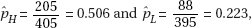 we have nHH = 205, nH(1 – H) = 200, nLL = 88, and nL(1 – L) = 307. These are all greater than 10.
Calculate the test statistic and the P-value:
Calculator software (such as 2-PropZTest on the TI-84) gives z = 8.318 and P = 0.0000.
State the conclusion in context with linkage to the P-value:
With this small a P-value, 0.0000 < 0.0001, there is very strong evidence to reject H0. That is, there is very strong evidence that a greater proportion of patients receiving higher doses experience severe nausea than patients receiving lower doses.
(b) Identify the confidence interval by name or formula:
95% confidence interval for the slope of the regression line b ± tsb
Check the assumptions:
The scatterplot is roughly linear, there is no apparent pattern in the residuals plot, and the distribution of the residuals is approximately normal (because the normal probability plot is roughly linear).
Calculate the confidence interval:
df = n – 2 = 8 – 2 = 6
0.006659 ± 2.447(0.001761) = 0.006659 ± 0.004309
(0.00235, 0.010968)
Interpret the confidence interval in context:
We are 95% confident that the mean proportion of patients experiencing severe nausea goes up between 0.00235 and 0.010968 with each increase of 1 milligram per week in dose intensity.
(c) The probability that a randomly chosen patient experienced severe nausea is  so the probability that at least 3 out of 5 experienced severe nausea is
SCORING
Part (a) has four parts: 1) stating the hypotheses; 2) identifying the test and checking assumptions; 3) calculating the test statistic and the P-value; and 4) giving a conclusion in context with linkage to the P-value. Part (a) is essentially correct if three or four of these parts are correct and partially correct if one or two of these parts are correct.
Part (b) has four parts: 1) identifying the confidence interval; 2) checking assumptions; 3) calculating the confidence interval; and 4) interpreting the confidence interval in context. Part (b) is essentially correct if three or four of these parts are correct and partially correct if one or two of these parts are correct.
Part (c) is essentially correct if the correct probability is calculated and the derivation is clear. Part (c) is partially correct for indicating a binomial with n = 5 and p = 0.366, but then calculating incorrectly.
4 Complete Answer |
All three parts essentially correct. |
3 Substantial Answer |
Two parts essentially correct and one part partially correct. |
2 Developing Answer |
Two parts essentially correct OR one part essentially correct and one or two parts partially correct OR all three parts partially correct. |
1 Minimal Answer |
One part essentially correct OR two parts partially correct. |
Practice Examination 4
SECTION I
1. (A) The slope, 6.2, gives the predicted increase in the y-variable for each unit increase in the x-variable.
2. (E) For a simple random sample, every possible group of the given size has to be equally likely to be selected, and this is not true here. For example, with this procedure it will be impossible for all the early arrivals to be together in the final sample. This procedure is an example of systematic sampling, but systematic sampling does not result in simple random samples.
3. (C) Power = 1 –  , and is smallest when
  is more and n is more.
4. (B) The critical z-scores for 60% to the right and 70% to the left are –0.253 and 0.524, respectively. Then {µ – 0.253 = 3, µ + 0.524 = 6} gives µ = 3.977 and = 3.861.
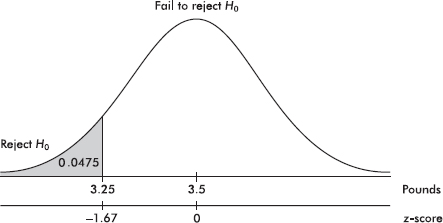
5. (A) We have H0: µ = 3.5 and Ha: µ < 3.5. Then 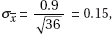 the z-score of 3.25 is
 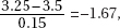 and Table A gives 0.0475. (A t-test on the TI-84 gives 0.0522.)
6. (A) The cumulative proportions of 0.25 and 0.75 correspond to Q1 = 57 and Q3 = 75, respectively, and so the interquartile range is 75 – 57 = 18.
7. (C) A placebo is a control treatment in which members of the control group do not realize whether or not they are receiving the experimental treatment.
8. (E) In experiments on people, subjects can be used as their own controls, with responses noted before and after the treatment. However, with such designs there is always the danger of a placebo effect. In this case, subjects might well have slower reaction times after drinking the alcohol because they think they should. Thus the design of choice would involve a separate control group to use for comparison. Blocking is not necessary for a well-designed experiment, and there is no indication that it would be useful here.
9. (E) Since (–2, 4) is on the line = 7x + b, we have 4 = –14 + b and b = 18. Thus the regression line is = 7x + 18. The point (x, y) is always on the regression line, and so we have y = 7x + 18.
10. (A) A simple random sample can be any size.
11. (E) With such small populations, censuses instead of samples are used, and there is no resulting probability statement about the difference.
12. (C) Half the area is on either side of 23, so 23 is the median. The distribution is skewed to the right, and so the mean is greater than the median. With half the area to each side of 23, half the applicants’ ages are to each side of 23. Histograms such as this show relative frequencies, not actual frequencies.
13. (B) While the procedure does use some element of chance, all possible groups of size 75 do not have the same chance of being picked, so the result is not a simple random sample. There is a real chance of selection bias. For example, a number of relatives with the same name and all using the same long-distance carrier might be selected.
14. (C) While t-distributions do have mean 0, their standard deviations are greater than 1.
15. (E)
16. (E) The critical z-scores are  with corresponding right tail probabilities of 0.3372 and 0.0188. The probability of being less than 100,000 given that the mileage is over 80,000 is
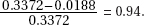
17. (A) 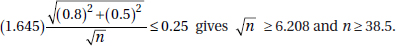
18. (A) The correlation coefficient is not changed by adding the same number to every value of one of the variables, by multiplying every value of one of the variables by the same positive number, or by interchanging the x- and y-variables.
19. (A) The binomial distribution with n = 2 and p = 0.8 is P(0) = (0.2)2 = 0.04, P(1) = 2(0.2) (0.8) = 0.32, and P(2) = (0.8)2 = 0.64, resulting in expected numbers of 0.04(200) = 8, 0.32(200) = 64, and 0.64(200) = 128. Thus,
20. (D) Option II gives the highest expected return: (50,000)(0.5) + (10,000)(0.5) = 30,000, which is greater than 25,000 and is also greater than (100,000)(0.05) = 5000. Option I guarantees that the $20,000 loan will be paid off. Option III provides the only chance of paying off the $80,000 loan. The moral is that the highest expected value is not automatically the “best” answer.
21. (B)
22. (E) This study is an experiment because a treatment (extensive exercise) is imposed. There is no blinding because subjects clearly know whether or not they are exercising. There is no blocking because subjects are not divided into blocks before random assignment to treatments. For example, blocking would have been used if subjects had been separated by gender or age before random assignment to exercise or not.
23. (C) From the shape of the normal curve, the answer is in the middle. The middle two-thirds is between z-scores of ±0.97, and 35 ± 0.97(10) gives (25.3, 44.7).
24. (B) The interquartile range is the length of the box, so they are not all equal. More than 25% of the patients in the A group had over 210 minutes of pain relief, which is not the case for the other two groups. There is no way to positively conclude a normal distribution from a boxplot.
25. (B) A scatterplot would be horizontal; the correlation is zero.
26. (D) 
27. (E) The midpoint of the confidence interval is 0.08.
28. (D) Increasing the sample size by a multiple of d2 divides the standard deviation of the set of sample means by d.
29. (A) With df = 43.43 and t = –3.94, the P-value is 0.000146 < 0.01. [On the TI-84, use tcdf.]
30. (D) While the sample proportion is between 64% and 70% (more specifically, it is 67%), this is not the meaning of ±3%. While the percentage of the entire population is likely to be between 64% and 70%, this is not known for certain.
31. (B) In this binomial situation, the probability that a car does not receive a ticket is 1 – 3 = 0.7, the probability that none of the five cars receives a ticket is (0.7)5, and thus the probability that at least one receives a ticket is 1 – (0.7)5.
32. (A) 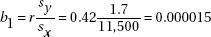
33. (B) If the standard deviation of a set is zero, all the values in the set are equal. The mean and median would both equal this common value and so would equal each other. If all the values are equal, there are no outliers. Just because the sample happens to have one common value, there is no reason for this to be true for the whole population. Statistics from one sample can be different from statistics from any other sample.
34. (A) The first study is an experiment with two treatment groups and no control group. The second study is observational; the researcher did not randomly divide the subjects into groups and have each group watch a designated number of hours of television per night.
35. (E) This refers only to very particular random variables, for example, random variables whose values are the numbers of successes in a binomial probability distribution with large n.
36. (B) A Type I error means that the null hypothesis is correct (the weather will remain dry), but you reject it (thus you needlessly carry around an umbrella). A Type II error means that the null hypothesis is wrong (it will rain), but you fail to reject it (thus you get drenched).
37. (E) If the sample statistic is far enough away from the claimed population parameter, we say that there is sufficient evidence to reject the null hypothesis. In this case the null hypothesis is that µ = 9500. The P-value is the probability of obtaining a sample statistic as extreme as the one obtained if the null hypothesis is assumed to be true. The smaller the P-value, the more significant the difference between the null hypothesis and the sample results. With P = 0.0069, there is strong evidence to reject H0.
38. (E) There are 10 + 12 = 22 students in the combined group. In ascending order, where are the two middle scores? At least 5 third graders and 6 fourth graders have heights less than or equal to 49 inches, so at most 11 students have heights greater than or equal to 49 and thus the median is less than or equal to 49. At least 5 third graders and 6 fourth graders have heights greater than or equal to 47 inches, so at most 11 students have heights less than or equal to 47 and thus the median is greater than or equal to 47. All that can be said about the median of the combined group is that it is between 47 and 49 inches.
39. (E) Good experimental design aims to give each group the same experiences except for the treatment under consideration, Thus, all three SRSs should be picked from the same grade level.
40. (E) The stemplot does not indicate what happened for any individual school.
SECTION II
1. (a) This is an example of stratified sampling, where the chapters are strata. The advantage is that the student is ensuring that the final sample will represent the 12 different authors, who may well use different average word lengths.
(b) This is an example of cluster sampling, where for each chapter the three chosen pages are clusters. It is reasonable to assume that each page (cluster) resembles the author’s overall pattern. The advantage is that using these clusters is much more practical than trying to sample from among all an author’s words.
(c) This is an example of systematic sampling, which is quicker and easier than many other procedures. A possible disadvantage is that if ordering is related to the variable under consideration, this procedure will likely result in an unrepresentative sample. For example, in this study if an author’s word length is related to word order in sentences, the student could end up with words of particular lengths.
SCORING
Part (a) is essentially correct for identifying the procedure and giving a correct advantage. Part (a) is partially correct for one of these two elements.
Part (b) is essentially correct for identifying the procedure and giving a correct advantage. Part (b) is partially correct for one of these two elements.
Part (c) is essentially correct for identifying the procedure and giving a correct disadvantage. Part (c) is partially correct for one of these two elements.
4 Complete Answer |
All three parts essentially correct. |
3 Substantial Answer |
Two parts essentially correct and one part partially correct. |
2 Developing Answer |
Two parts essentially correct OR one part essentially correct and one or two parts partially correct OR all three parts partially correct. |
1 Minimal Answer |
One part essentially correct OR two parts partially correct. |
2. (a) The SRS with n = 50 is more likely to have a sample proportion greater than 75%. In each case, the sampling distribution of is approximately normal with a mean of 0.69 and a standard deviation of 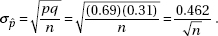 Thus the sampling distribution with n = 50 will have more variability than the sampling distribution with n = 100. Thus the tail area ( > 0.75) will be larger for n = 50.
(b) The size of the sample, 30, is much too large compared to the size of the population, 95. With a sample size this close to the population size, the necessary assumption of independence does not follow. A commonly accepted condition is that the sample should be no more than 10% of the population.
(c) A normal distribution may be used to approximate a binomial distribution only if the sample size n is not too small. The commonly used condition check is that both np and nq are at least 10. In this case nq = (20)(1 – 0.78) = 4.4.
SCORING
Part (a) is essentially correct for correctly giving n = 50 and linking in context to variability in the sampling distributions. Part (a) is partially correct for a correct answer missing comparison of variability in the sampling distributions.
Part (b) is essentially correct for a clear explanation in context. Part (b) is partially correct for saying the sample size is too close to the population size but not linking to this context (sample size 30 and population size 95).
Part (c) is essentially correct for a clear explanation in context. Part (c) is partially correct for saying the sample size is too small but not linking to this context (nq = 4.4 < 10).
4 Complete Answer |
All three parts essentially correct. |
3 Substantial Answer |
Two parts essentially correct and one part partially correct. |
2 Developing Answer |
Two parts essentially correct OR one part essentially correct and one or two parts partially correct OR all three parts partially correct. |
1 Minimal Answer |
One part essentially correct OR two parts partially correct. |
3. (a) The value 50.90 estimates the average score of males who spend 0 hours studying. The value 9.45 estimates the average increase in score for each additional hour study time. For any fixed number of hours study time, the value 4.40 estimates the average number of points that females score higher than males.
(b)
(c) For each additional hour of study time, the scores of males increase an average of 8.5 while those of females increase an average of 10.4. Additional hours of study time appear to benefit females more than males, something that does not show in the original model.
(d)
SCORING
Part (a) is essentially correct for correctly interpreting all three numbers in context and partially correct for correctly interpreting two of the three numbers.
Part (b) is essentially correct for correct graphs, clearly parallel and labeled as to which is which. Part (b) is partially correct for correct parallel graphs but missing labels, or for labeled, parallel graphs with incorrect y-intercepts.
Part (c) is essentially correct for correctly interpreting both slopes and for some comparative statement about additional hours study time appearing to benefit females more than males. Part (c) is partially correct for correctly interpreting both slopes but failing to make a comparative statement, or for making a correct comparative statement without interpreting the slopes.
Part (d) is essentially correct for correct graphs, clearly showing different slopes and labeled as to which is which. Part (d) is partially correct for graphs, clearly showing different slopes but missing labels, or for labeled graphs with different slopes but with incorrect y-intercepts.
Count partially correct answers as one-half an essentially correct answer.
4 Complete Answer |
Four essentially correct answers. |
3 Substantial Answer |
Three essentially correct answers. |
2 Developing Answer |
Two essentially correct answers. |
1 Minimal Answer |
One essentially correct answer. |
Use a holistic approach to decide a score totaling between two numbers.
4. (a) Name the procedure: This is a one-sample t-interval for the mean.
Check the conditions: We are given that this is a random sample, n = 5 is less than 10% of all vials of this product, and a dotplot
makes the nearly normal condition reasonable.
Mechanics: Putting the data in a List, calculator software (such as TInterval on the TI-84) gives (2.4674, 2.6966).
Conclusion in context: We are 95% confident that the mean concentration level for the active ingredient found in this pharmaceutical product is between 2.467 and 2.697 milligrams per milliliter.
(b) Raising the confidence level would increase the width of the confidence interval.
(c) Since the whole confidence interval (2.467, 2.697) is below the critical 2.7, at the 95% confidence level the mean concentration is at a safe level. However, with 2.697 so close to 2.7, based on the statement in (c), if the confidence level is raised we are no longer confident that the mean concentration is at a safe level.
SCORING
Part (a) has two components. The first component is essentially correct for correctly naming the procedure and checking the conditions, and is partially correct for one of these two. The second component is essentially correct for correct mechanics and a correct conclusion in context, and is partially correct for one of these two.
Part (b) is either essentially correct or incorrect.
Part (c) is essentially correct for a correct conclusion in context for both the 95% interval and for if the confidence is raised, both conclusions referencing the answers from (a) and (b). Part (c) is partially correct for a correct conclusion in context for either of the confidence intervals or for both but with a weak explanation.
Count partially correct answers as one-half an essentially correct answer.
4 Complete Answer |
Four essentially correct answers. |
3 Substantial Answer |
Three essentially correct answers. |
2 Developing Answer |
Two essentially correct answers. |
1 Minimal Answer |
One essentially correct answer. |
Use a holistic approach to decide a score totaling between two numbers.
5. (a) Points A and B both have high leverage; that is, both their x-coordinates are outliers in the x-direction. However, point B is influential (its removal sharply changes the regression line), while point A is not influential (it lies directly on the regression line, so its removal will not change the line).
(b) Point C lies off the regression line so its residual is much greater than that of point D, whose residual is 0 (point D lies on the regression line). However, the removal of point C will very minimally affect the slope of the regression line, if at all, while the removal of point D dramatically affects the slope of the regression line.
(c) Removal of either point E or point F minimally affects the regression line, while removal of both has a dramatic effect.
(d) Removing either point G or point H will definitely affect the regression line (pulling the line toward the remaining of the two points), while removing both will have little, if any, effect on the line.
SCORING
Each of parts (a), (b), (c), and (d) has two components and is scored essentially correct for both components correct and partially correct for one component correct.
Give 1 point for each essentially correct part and  point for each partially correct part.
Count partially correct answers as one-half an essentially correct answer.
4 Complete Answer |
4 points |
3 Substantial Answer |
3 points |
2 Developing Answer |
2 points |
1 Minimal Answer |
1 point |
Use a holistic approach to decide a score totaling between two numbers.
SECTION II
Part B
6. (a) State the hypotheses: H0: µA – µB = 0 and Ha: µA – µB ≠ 0
Identify the test and check conditions: two-sample t-test. It is given that the samples are random, and we assume n = 390 and n = 235 are less than 10% of the adult populations of the two communities. The populations may not be normal, but since nA = 390 and nB = 235 are both large, it is OK to proceed with the t-test.
Calculate the test statistic t and the P-value: calculator software (such as 2-SampTTest on the TI-84) gives t = –1.528 and P = 0.1272 using the data, or t = –1.515 and P = 0.1306 using the summary statistics.
Conclusion in context: With this large a P-value, 0.13 > 0.05, there is not sufficient evidence to reject H0, that is, there is not sufficient evidence of a difference in the mean years of schooling between the two communities.
(b) State the hypotheses: H0: The distribution of years of schooling is the same in the two communities. Ha: The distribution of years of schooling is not the same in the two communities.
Identify the test and check conditions: Chi-square test (of homogeneity). All expected counts are > 5.
Calculate the test statistic and the P-value:  2 = 57.85 and with df = (7 – 1)(2 – 1) = 6, we have P = 0.000.
State the conclusion in context: With this small a P-value, 0.000 < 0.05, there is sufficient evidence to reject H0, that is, there is strong evidence that the distribution of years of schooling is not the same in the two communities.
(c)
Although the two distributions have roughly the same center, their shapes are different. The distribution of years of schooling for Community A is unimodal, symmetric, and bell-shaped, while that of Community B is roughly bimodal with few scores in the center.
SCORING
Part (a) is essentially correct if all four steps for a two-sample t-test are correct and partially correct if three steps are correct.
Part (b) is essentially correct if all four steps for a chi-square test (of homogeneity) are correct and partially correct if three steps are correct.
Part (c) is essentially correct for an accurate comparison of the distributions linked to correctly drawn histograms. Part (c) is partially correct if only one of the two parts (comparison and histograms) is correct or if both are correct but there is no linkage.
4 Complete Answer |
All three parts essentially correct. |
3 Substantial Answer |
Two parts essentially correct and one part partially correct. |
2 Developing Answer |
Two parts essentially correct OR one part essentially correct and one or two parts partially correct OR all three parts partially correct. |
1 Minimal Answer |
One part essentially correct OR two parts partially correct. |
Practice Examination 5
SECTION I
1. (B) µx = µ = 8, and 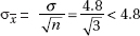
2. (E) None of the studies have any controls such as randomization, a control group, or blinding, and so while they may give valuable information, they cannot establish cause and effect.
3. (C) The range increased from 90 – 15 = 75 to 97 – 21 = 76, while the standard deviation decreased (note how the values are bunched together more closely in 1998).
4. (E) 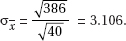 The critical z-scores are
 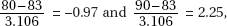 resulting in a probability of 0.3340 + 0.4878 = 0.8218.
5. (D) The critical z-scores are 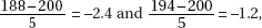 with corresponding left tail probabilities of 0.0082 and 0.1151, respectively. The probability of being greater than 188 given that it is less than 194 is
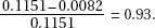
6. (C)
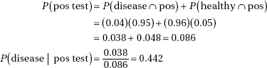
7. (D) Given a census, the population parameter is known, and there is no need to use the techniques of inference.
8. (C) Sixty-four percent of the students scored below Mary and 56% scored below Pam, and so 8% must have scored between them.
9. (E) Intentionally forcing some treatment to note the response is associated with controlled experiments, not with observational studies. In experiments, the researchers decide how people are placed in different groups; self-selection is associated with observational studies. Results of observational studies may suggest cause-and-effect relationships; however, controlled studies are used to establish such relationships.
10. (E) With  the greater the sample size n, the smaller the standard deviation σx.
11. (D) df = 9, and 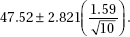
12. (E) The set could be {150, 150, 150, 200} with mean 162.5 and median 150. It might also be {150, 200, 200, 200} with mean 187.5 and median 200. The median of a set of four elements is the mean of the two middle elements.
13. (D) 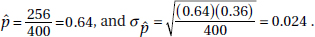 The z-scores of 0.60 and 0.68 are
 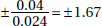 for a probability of 0.9525 – 0.0475 = 0.9050.
14. (C) This is a binomial with n = 15 and p = 0.29, and so the mean is np = 15(0.29) = 4.35.
15. (D) With independence, variances add, so 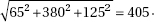
16. (E) Without independence we cannot determine var(X + Y) from the information given.
17. (A) Bias is the tendency to favor the selection of certain members of a population. It has nothing to do with the shape of distributions. The natural variability between samples is called sampling error.
18. (C) There are not two distinct peaks, so the distribution is not bimodal. Relative frequency is given by relative area. The distribution is skewed to the left, and so the mean is less than the median.
19. (D) While the standard deviation of the z-distribution is 1, the standard deviation of the t-distribution is greater than 1.
20. (B)
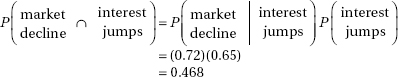
21. (E) Different samples give different sample statistics, all of which are estimates for the same population parameter, and so error, called sampling error, is naturally present.
22. (C) With four-digit accuracy as found on the TI-83, the critical z-scores for 70% to the right and 80% to the right are –0.5244 and –0.8416, respectively. Then {µ – 0.5244 = 12,000, µ – 0.8416 = 10,000} gives µ = 15,306 and = 6305. Using two-digit accuracy as found in Table A, that is, –0.52 and –0.84, results in µ = 15,250 and = 6250.
23. (D) The percentage of the variation in y explained by the variation in x is given by the coefficient of determination r2. In this example, (0.78)2 = 0.61.
24. (B) There is a weak negative correlation, and so –0.15 is the only reasonable possibility among the choices given.
25. (E) There is no guarantee that 24 is anywhere near the interval, and so none of the statements is true.
26. (E) Sampling error relates to natural variation between samples, and it can never be eliminated. In good observational studies, responses are not influenced during the collection of data. In good experiments, treatments are compared as to the differences in responses.
27. (E) The scatterplot suggests a zero correlation.
28. (A) 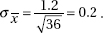 The z-score of 2.5 is
  and to the right of 2.5 is the probability of failing to reject the false claim.
29. (E) The central limit theorem says that no matter how the original population is distributed, as the sample size increases, the sampling distribution of the sample mean becomes closer to a normal distribution.
30. (D) A sampling distribution is the distribution of all the values taken by a statistic, such as sample mean or sample proportion, from all possible samples of a given size.
31. (E) P(at least 2) = P(exactly 2) + P(exactly 3) = 3(0.8)2(0.2) + (0.8)3
32. (A) The critical t-scores for 99% confidence with df = 6 are ±3.707.
33. (B) The PTA survey has strong response bias in that students may not give truthful responses to a parent or teacher about their engaging in unprotected sex. The talk show survey results in a voluntary response sample, which typically gives too much emphasis to persons with strong opinions. The Ladies Home Journal survey has strong selection bias; that is, people who read the Journal are not representative of the general population.
34. (D) To divide the interval estimate by d, the sample size must be increased by a multiple of d2.
35. (B) P(0 pts) = (0.05)2, P( pt) = 2(0.05)(0.15), P(1 pt) = (0.15)2 + 2(0.05)(0.8), P(1 pts) = 2(0.15)(0.8), and P(2 pts) = (0.8)2.
36. (A) The P-value is the probability of obtaining a result as extreme as the one seen given that the null hypothesis is true; thus it is a conditional probability. The P-value depends on the sample chosen. The P-value in a two-sided test is calculated by doubling the indicated tail probability. P-values are not restricted to use with any particular distribution. With a small P-value, there is evidence to reject the null hypothesis, but we’re not proving anything.
37. (C) A Type II error is a mistaken failure to reject a false null hypothesis or, in this case, a failure to realize that the machinery is turning out wrong size ball bearings.
38. (E) Using a measurement from a sample, we are never able to say exactly what a population mean is; rather we always say we have a certain confidence that the population mean lies in a particular interval. In this case we are 95% confident that Lipitor will outperform niacin by 18 to 41 points.
39. (C) The median number of hours is less than four for June, July, and August.
40. (D) A horizontal line drawn at the 0.9 probability level corresponds to roughly 19 rooms.
SECTION II
Part A
1. (a) In each block, two of the sites will be randomly assigned to receive Type A vegetation, while the remaining two sites in the block will receive Type B vegetation. Randomization of vegetation type to the sites within each block should reduce bias due to any confounding variables. In particular, the randomization in blocks in the first scheme should even out the effect of the distance vegetation in blocks is from the industrial park.
(b) The first scheme creates homogeneous blocks with respect to distance from the river, while the second scheme creates homogeneous blocks with respect to the industrial park. Randomization of vegetation types to sites within blocks in the first scheme should even out effects of distance from the industrial park, while randomization of vegetation types to sites within blocks in the second scheme should even out effects of distance from the river.
SCORING
It is important to explain why randomization is important within the context of this problem, so use of terms like bias and confounding must be in context. One must explain the importance of homogeneous experimental units (sites, not vegetation types) within blocks.
4 Complete Answer |
Correct explanation both of use of blocking and of use of randomization in context of this problem. |
3 Substantial Answer |
Correct explanation of use of either blocking or randomization in context and a weak explanation of the other. |
2 Developing Answer |
Correct explanation of use of either blocking or randomization in context OR weak explanations of both. |
1 Minimal Answer |
Weak explanation of either blocking or randomization in context. |
2. (a)
(b) While the percentages in both regions have roughly symmetric distributions, the percentages from Region A form a distinctly unimodal pattern, while those from Region B are distinctly bimodal. That is, in Region B the countries tended to show either a very low or a very high percentage, while in Region A most countries showed a percentage near the middle one.
(c) Either an argument can be made for Region A because Region B has so many countries with high percentages (for primary-school-age children enrolled in school), or an argument can be made for Region B because Region B has so many countries with low percentages.
(d) Data are already given on all the countries in the two regions. In doing inference, one uses sample statistics to estimate population parameters. If the data are actually the whole population, there is no point of a t-test.
SCORING
Part (a) is essentially correct for a correct stemplot (numbers in each row do not have to be in order) with labeling as to which side refers to which region. Part (a) is partially correct for a correct stemplot missing the labeling.
Part (b) is essentially correct for noting that the percentages from Region A form a distinctly unimodal pattern, while those from Region B are distinctly bimodal. Part (b) is partially correct for noting either the unimodal pattern from the Region A data or the bimodal pattern from the Region B data.
Part (c) is essentially correct for choosing either region and giving a reasonable argument for the choice. Part (c) is partially correct if the argument is weak. Part (c) is incorrect for no argument or an incorrect argument for the choice given.
Part (d) is essentially correct for explaining that inference is not proper when the data are the whole population. Part (d) is partially correct if the explanation is correct but weak.
Count partially correct answers as one-half an essentially correct answer.
4 Complete Answer |
Four essentially correct answers. |
3 Substantial Answer |
Three essentially correct answers. |
2 Developing Answer |
Two essentially correct answers. |
1 Minimal Answer |
One essentially correct answer. |
Use a holistic approach to decide a score totaling between two numbers.
3. (a) Note that there are a great number of values between 2.0 and 2.4, fewer values between 2.4 and 2.8, on down to the fewest values being between 3.6 and 4.0. Thus the distribution is skewed right (skewed toward the higher values).
(b) Note that the greatest five values, out of the 100 values, are above a point roughly at 3.4 or 3.5, so the 95th percentile is roughly 3.4 or 3.5.
(c) In a normal distribution, the 95th percentile has a z-score of 1.645. Reading up from the x-axis to the normal line and across to the y-axis gives a GPA of approximately 3.2.
SCORING
Part (a) is essentially correct if the shape is correctly identified as skewed right, and a correct explanation based on the given normal probability plot is given. Part (a) is partially correct for a correct identification with a weak explanation. Part (a) is incorrect if a correct identification is given with no explanation.
Part (b) is essentially correct for correctly noting 3.4 or 3.5 as the 95th percentile with a correct explanation. Part (b) is partially correct for giving 3.4 or 3.5 with a weak explanation or no explanation.
Part (c) is essentially correct for noting approximately 3.2 as the GPA and stating the method clearly. Part (c) is partially correct for giving 3.2 with a weak explanation or no explanation.
4 Complete Answer |
All three parts essentially correct. |
3 Substantial Answer |
Two parts essentially correct and one part partially correct. |
2 Developing Answer |
Two parts essentially correct OR one part essentially correct and one or two parts partially correct OR all three parts partially correct. |
1 Minimal Answer |
One part essentially correct OR two parts partially correct. |
4. (a) There are four elements to this solution.
State the hypotheses:
H0: The distribution of blood types among patients at this hospital is in the ratios of 9:8:2:1 for types O, A, B, and AB, respectively.
Ha: The distribution of blood types among patients at this hospital is not in the ratios of 9:8:2:1 for types O, A, B, and AB, respectively.
Identify the test by name or formula and check the assumptions:
Chi-square goodness-of-fit test:
Check the assumptions:
1. The researcher claims that the data are from a random sample of patient records.
2. The ratios 9:8:2:1 give expected cell frequencies of 
 each of which is at least 5.
Demonstrate correct mechanics:

With df = 4 – 1 = 3, the P-value is 0.0145.
State the conclusion in context with linkage to the P-value:
With this small a P-value, 0.145 < 0.05, there is sufficient evidence to reject H0, that is, there is sufficient evidence that the distribution of blood types among patients at this hospital is not in the ratios of 9:8:2:1 for types O, A, B, and AB, respectively.
(b) In this case the mechanics give:

With df = 4 – 1 = 3, the probability that 2 is less than or equal to 0.311 is 0.0421. With such a small probability, there is evidence that the data are too good to be true; that is, there is evidence that Researcher 2 made up the data to fit the 9:8:2:1 model.
SCORING
Part (a1) is essentially correct if the hypotheses are given, the test is identified, and the assumptions are checked. Part (a1) is partially correct for two of these three steps.
Part (a2) is essentially correct for correct mechanics and the conclusion given in context with linkage to the P-value. Part (a2) is partially correct if there is a minor error in mechanics OR the conclusion is not in context OR there is no linkage to the P-value.
Part (b) is essentially correct for noting that the probability of a 2 value of only 0.311 is very small, and thus the data are suspicious. Part (b) is partially correct for a correct idea but with a weak explanation.
4 Complete Answer |
All three parts essentially correct. |
3 Substantial Answer |
Two parts essentially correct and one part partially correct. |
2 Developing Answer |
Two parts essentially correct OR one part essentially correct and one or two parts partially correct OR all three parts partially correct. |
1 Minimal Answer |
One part essentially correct OR two parts partially correct. |
5. (a) The regression line is  liter.
Then 40.2462 – 4.61969(1.5) ≈ 33.32.
Residual = actual – predicted = 35 – 33.32 = 1.68
(b) The predicted value for mpg is 40.2462 – 4.61969(5.0) ≈ 17.15, which is very close to the actual value of 17. The added point is consistent with the linear pattern given by the computer output, so the new slope should be about the same as the old slope.
(c) Since the new point fits the old linear pattern so well, and has an x-value (liter) much greater than x = 2.52, the absolute value of the correlation will increase.
SCORING
Part (a) is essentially correct for a correct calculation of the residual. Part (a) is partially correct for noting that residual = actual – predicted, but obtaining an incorrect answer because of an incorrect derivation of the regression line.
Part (b) is essentially correct for showing that the actual value is very close to the predicted value and concluding that the new slope should be about the same. Part (b) is partially correct if the predicted value is miscalculated but a proper conclusion based on the miscalculation is reached.
Part (c) is essentially correct for concluding that the absolute value of the correlation will increase because the new point fits the old linear pattern so well. Part (c) is partially correct for concluding that the absolute value of the correlation will increase but giving a weak explanation.
4 Complete Answer |
All three parts essentially correct. |
3 Substantial Answer |
Two parts essentially correct and one part partially correct. |
2 Developing Answer |
Two parts essentially correct OR one part essentially correct and one or two parts partially correct OR all three parts partially correct. |
1 Minimal Answer |
One part essentially correct OR two parts partially correct. |
SECTION II
Part B
6. (a) State the hypotheses: H0: µd = 0 and Ha: µd > 0 where µd is the mean difference (2000 – 1990) in the populations of the southern states.
Identify the test: paired t-test.
Calculate the test statistic t and the P-value: calculator software (such as T-Test on the TI-84) gives t = 2.035 and P = 0.05578.
Conclusion in context with linkage to the P-value: With this large a P-value, 0.05578 > 0.05, there is not sufficient evidence to reject H0, that is, there is not sufficient evidence to conclude that southern states grew between 1990 and 2000.
(b) Identify the confidence interval: two-sample t-interval for µN – µS, the difference in mean populations between northern and southern states in 1990.
Mechanics: Calculator software (such as 2-SampTInt on the TI-84) gives (–9116, 10,458).
Interpretation in context: We are 95% confident that the true difference in the average populations of northern and southern states in 1990 was between –9116 and 10,458 thousand people.
(c) State the hypotheses: H0: µd = 0 and Ha: µd >0 where µd is the difference in the mean growths of populations of southern and northern states.
Identify the test: two-sample t-test.
Calculate the test statistic t and the P-value: Calculator software (such as 2-SampTTest on the TI-84) gives t = 1.229 and P = 0.1401.
Conclusion in context with linkage to the P-value: With this large a P-value, 0.1401 > 0.05, there is not sufficient evidence to reject H0, that is, there is not sufficient evidence that southern states grew faster than northern states between 1990 and 2000.
SCORING
Conditions for inference are assumed to be met and don’t have to be mentioned.
Part (a) is essentially correct if all four steps are correct and partially correct if three steps are correct.
Part (b) is essentially correct if all three steps are correct and partially correct if two steps are correct. Full credit for df = 4 or 8.
Part (c) is essentially correct if all four steps are correct and partially correct if three steps are correct. Full credit for df = 4, 4.43, or 8.
4 Complete Answer |
All three parts essentially correct. |
3 Substantial Answer |
Two parts essentially correct and one part partially correct. |
2 Developing Answer |
Two parts essentially correct OR one part essentially correct and one or two parts partially correct OR all three parts partially correct. |
1 Minimal Answer |
One part essentially correct OR two parts partially correct. |