Chapter 19
Hurricanes, Tornados, and Whirlpools

In this chapter, we take a brief look at the potential applicability of the fractional trigonometry and the fractional spiral functions to vortex flows such as hurricanes, tornados, and whirlpools. According to Buckley et al. [18] p. 66, “… vortices may originate either when a weak area of low pressure forms or when the overall wind regime encounters a barrier…” At this time, we examine the morphology of these phenomena and other weather phenomena such as low-pressure cloud patterns based on available images.

In the applications that follow, the computations of the spiral loci of Sections 19.1, 19.3, and 19.4 are based on the fractional meta-trigonometric - and -functions, and are identical to the mathematical definitions and nomenclature given in Section 18.3.4.

19.1 Hurricane Cloud Patterns

Modern satellite technology has provided a new perspective into the morphology of hurricane flows. This allows the potential application of the fractional trigonometric spirals to the mapping of streamlines observed in cloud structures. In this section, we consider the morphology of the cloud patterns that are characteristic of the behavior of hurricane flows; see, for example, Kerry [33]. As discussed in the previous chapters, this is achieved by fitting fractional spirals to hurricane images and thus spatial modeling is possible. The parameters given for the spiral fits are the same as those used for the galaxy study in Chapter 18.

19.1.1 Hurricane Fran

Figure 19.1 is a satellite image of hurricane Fran off of the coast of Florida taken in September 1996. Several of the major flow patterns have been fit to the image. The fitting parameters are summarized in Table 19.1. With the exception of Leg 2, the legs are all fit well with order parameters q = 0.45 and v = 0.0. The fit for Leg 2 using q = 0.45 was only slightly inferior to that used in the table.

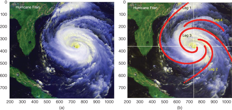
Figure 19.1 Hurricane Fran off the Florida coast. (a) Reference image, (b) model. See text for spiral parameters.

Source: NASA GSFC. Public domain. Please see www.wiley.com/go/Lorenzo/Fractional_Trigonometry for a color version of this figure.

Table 19.1 Fitting parameters for Hurricane Fran

Leg	q	v							C
1	0.45	0	0.20	0.80	40	0	90		220
2	0.35	0	0.20	0.80	0	40	−100		120
3	0.45	0	0.20	0.80	40	0	−30		170
4	0.45	0	0.20	0.80	40	0	−90		120

19.1.2 Hurricane Isabel

The form of hurricane Isabel, off the east coast of the United States in September 2003 (as seen in Figure 19.2) appears to be quite symmetric. This is possibly due to its distance from land. In this study, it was decided to attempt a fully symmetric fit, which is shown. In this figure, the six spirals seen are the primary spiral and five identical spirals symmetrically spaced about the origin, which is at the center of the hurricane eye. The parameters for this model were q = 0.48, v = 0, a = 1, , , , , , C = 1500, and .

Figure 19.2 Hurricane Isabel. (a) Hurricane Isabel reference image, (b) model. See text for spiral parameters.

Source: NASA. Public domain. Please see www.wiley.com/go/Lorenzo/Fractional_Trigonometry for a color version of this figure.

In the magnified view of Figure 19.3, the spirals were extended by continuing to expose the morphology entering the eye. Relative to the set of parameters quoted for this spiral, it was found that changing the order parameter q to q = 0.5 resulted in coalescence of the spirals into an exact circle. However, q = 0.48 provided a better match for the streamline morphology.

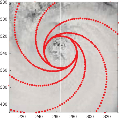
Figure 19.3 Magnified view of Hurricane Isabel showing eye and fit of extended streams. See text for parameters. Please see www.wiley.com/go/Lorenzo/Fractional_Trigonometry for a color version of this figure.

It is important to note for both cases studied that , the parametric variable along each streamline, is interpreted as a spatial variable. In the fittings, this variable increases as the eye is approached. At the upper level of the hurricane, it is thought that the direction of rotation reverses into an outflow jet (Emanuel [33], p. 16). Such a reversal is not apparent in these images. The cloud structure seen appears to be that associated with the inflow of the lower level of the hurricane.

The fractional trigonometric order for a hurricane is likely a variable-order process (Lorenzo and Hartley [72]), that is, q<1 for the inflow transitioning to q approximately unity for the helical up-flow at the eye wall, and further increasing to q>1 for the unstable outflow at the top of the vortex. The differential order of the associated fractional differential equations will be twice the trigonometric order for the fractional sine and cosine. This can be seen from the Laplace transforms for the functions.

19.2 Tornado Classification

With tornadic flows, it is not currently possible to obtain images looking along the axis of rotation exposing the circular or spiral nature of the flow. However, images are often available showing tornado profiles. The current classification for tornados is the Enhanced Fujita scale, the EF scale. The Fujita scale, Bluestein [17], p. 5, is based on the nature of the damage that is observed after the event and a wind speed range is associated with each of the scale elements. For example, an EF-5 tornado is estimated to have winds in excess of 200 miles per hour. In this study, the fractional trigonometric function k index will be used as the basis for a possible classification of tornadic forms based on their profiles.

19.2.1 The k Index

The fractional trigonometric functions by their definitions,

19.1

19.2

are indexed by the variable k, where and is the product of the denominators of the rational arguments , , , and with D in minimal form. The source of this indexing is the fractional exponent , which leads to the arguments for the sine and cosine in the definitions of the meta-trigonometric functions. When these functions occur as the solutions to fractional differential equations, the various values of k lead to equivalent solutions. However, as we have seen in Chapters 7–9, the functions are different when viewed individually.

In the near-order effect (Section 14.7), one or more of the denominators becomes large, leading to a large value for k. For properly selected functions, this can be utilized for the classification of tornado profile morphology.

19.2.2 Tornado Morphology Animation

A very-much simplified simulation of a tornado is shown in Figure 19.4. The animation is done in Matlab® (version R2012a) and is based on the R₂-trigonometric functions with height h, replacing t as the main variable. To study the tornado profile, the order q was set at q = 48/49, v = 0, and 12 equally spaced streams (functions) are set into rotation. The figure shows a fixed time slice in a 3D plot. Note that the R₂-functions may be written in terms of the meta-trigonometric functions, for example, . The program for the simulation is given in Appendix C.

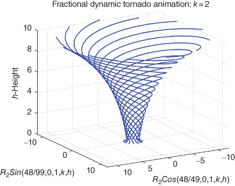
Figure 19.4 Simplified tornado model, 3D time slice.

19.2.3 Tornado Morphology Classification

If the index is allowed to vary, the profile morphology varies as shown in the sequence of panels of Figure 19.5. As can be seen in the sequence, as the index variable k increases, the change in radius with height, , also increases and subjectively the strength of the tornado increases. The fineness of such a classification system can be readily increased by increasing the size of the denominator . In Figure 19.6, the value of is increased from q = 48/49, by setting q = 98/99. With q = 98/99 and the new index k = 1, this clearly yields a morphology that interpolates between k = 0 and k = 1 in the q = 48/49 system and includes these points as k = 0 and k = 2 in the refined q = 98/99 based system.

Figure 19.5 Tornado morphology as function of k index, for q = 48/49, v = 0, and k = 0, 1, 2, 3, 4. (a) k = 0, (b) k = 1, (c) k = 2, (d) k = 3, (e) k = 4.

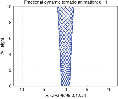
Figure 19.6 Tornado morphology k = 1, for q = 98/99.

Two additional features are desired for a classification system based on these functions. First, for the morphologies shown in Figure 19.5, the footprint of the tornadoes is set by choosing the raw or unmultiplied functions. Clearly, the larger the footprint is, the more severe the tornado. This can be accommodated by multiplying the fractional trigonometric functions by an appropriate factor depending on k. For example, . This assumes that severity increases as increases. Furthermore, such a factor, of course, will change with the choice of . Also, a choice of D_q must be made to provide satisfactory resolution particularly for the weaker tornados. Second, the velocity at or near ground level should be keyed to the index value to calibrate the classification system. This of course will require observational input. These last steps are beyond the scope of this effort.

Application of the tornado morphology classification scheme requires tornado profile images that are at least roughly size calibrated. From such images, dr/dh versus h and the tornado footprint may be estimated, and this information can be used to classify the tornado.

19.3 Low-Pressure Cloud Pattern

A rather phenomenal satellite image of the cloud pattern of a low-pressure system over Iceland is of significant interest relative to the fractional trigonometric spirals. The question being: could fractional spirals be found that are representative of the flow pattern inferred by the cloud structure? Figure 19.7 shows the reference image along with two images showing a fractional spiral model and a close-up view of the center of the spiral. The fractional spiral provides a good representation over a significant number of rotations of the spiral. The two spirals shown are scaled and rotated versions of each other, and the spiral parameters are q = 0.90, v = 0.0, a = 1.0, , , , for both spirals. For the inner spiral, C = 1100, , and for the outer spiral, C = 1680, .

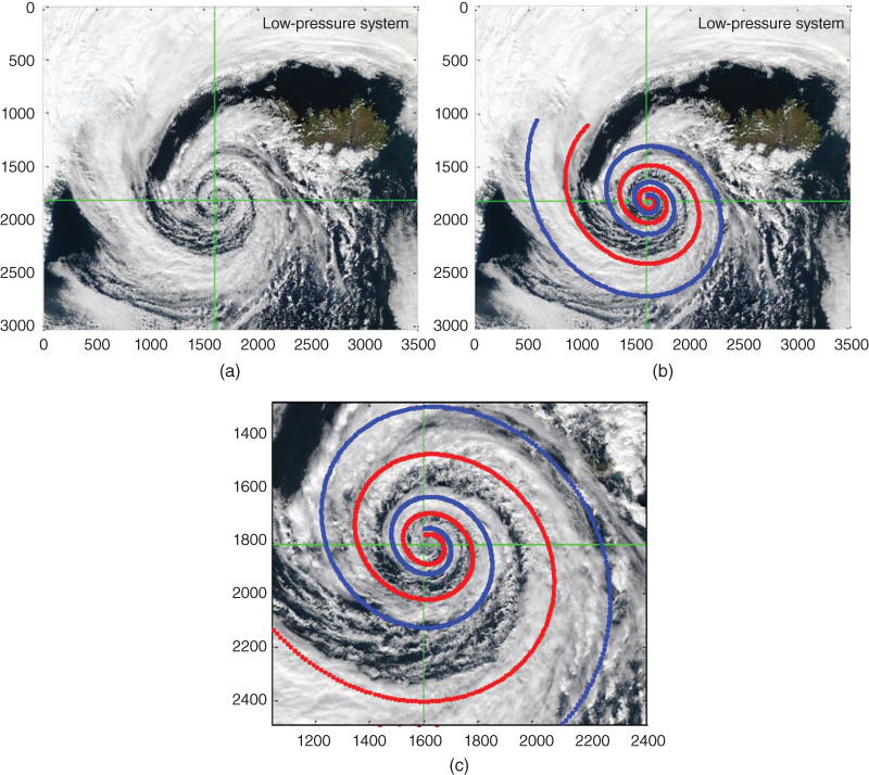
Figure 19.7 Low-pressure system over Iceland. (a) Reference view, (b) fractional spiral model, and (c) fractional model enlarged. See text for spiral parameters.

Source: NASA. Public domain. Please see www.wiley.com/go/Lorenzo/Fractional_Trigonometry for a color version of this figure.

19.4 Whirlpool

Associated with the disastrous tsunami that struck Japan in March 2011, an enormous whirlpool was formed off the east coast of Japan near the port in Oaraj, Ibaraki Prefecture. The scale of the whirlpool may be judged by the ship seen in the image (Figure 19.8) and located on the x axis at x = 200. The morphology of the whirlpool is slightly deformed by the adjacent land masses; however, it is of considerable interest to evaluate the applicability of the fractional trigonometric spirals to this phenomenon. Three streamlines were fit for this model. The common parameters for the three legs are v = 0, a = 1, , , k = 0, . The remaining parameters are given in Table 19.2.

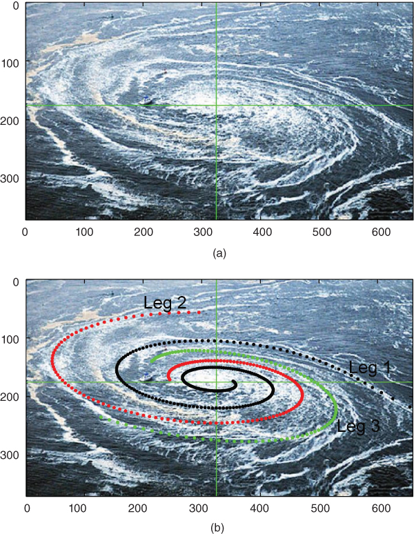
Figure 19.8 Whirlpool off the coast of Japan, March 2011. (a) Reference image, (b) fractional spiral model. See text for model parameters.

Source: Reuters Pictures. Reproduced with permission of Reuters. Please see www.wiley.com/go/Lorenzo/Fractional_Trigonometry for a color version of this figure.

Table 19.2 Parameters for Whirlpool model

Leg	q			C
1	0.65			180
2	0.62			300
3	0.62			425

In spite of the deformation caused by the adjacent land masses, the fractional spirals provided good fidelity to the visible streamlines.

19.5 Order in Physical Systems

In this and the previous two chapters, we have studied the applicability of the fractional spirals, and by inference the fractional trigonometric functions, to various physical and biological systems. While it is premature to draw any definitive conclusions, the following observations are forwarded. All of the studies were based on the complexity functions, the fractional sine and cosine, as applied to the spatial behavior of the processes involved. Only in the case of the Nautilus, were we able to use a modicum of auxiliary data to extend our understanding to a dynamic model that inferred the growth rate of the animal from conception to maturity. Such extensions, in general, are beyond the scope of the current effort. However, in Chapter 20, we suggest possible extension into this domain. It is of interest to consider the nature of the order variable, q, on the behavior of the processes. However, we digress briefly, to note the following. First, there two types of order: there is the order of the trigonometric functions, q that has been discussed in many places in the book. Second, there is the order of the associated fractional differential equations, that we abbreviate as the differential order, and use the notation, u. Based on the Laplace transforms (Section 9.4 and Table 9.1), the associated differential order for the complexity functions, the fractional sine and cosine, is given by u = 2q, and for the parity functions by u = 4q.

Table 19.3 summarizes the order associated with the fractional spirals used to fit the various morphologies. The stability listings in the table are computed based on equation (13.36) and relate to the spatial character of the morphologies. It should be noted for the whirlpool case that to four decimal places the computation yielded neutral stability.

Table 19.3 Order and spatial stability associated with various physical processes

Process	Trig. order	Differential order	Stability
Naut.& Shells	q >1	u >2	Unstable
Galaxies	q >1	u >2	Unstable
Hurricane inflows			Stable
Low pressure	q = 0.9	u = 1.8	Stable
Whirlpool	q = 0.62–0.65	u = 1.24–1.30	Stable

The unstable result for the sea shells is not surprising, for clearly a growth process is an unstable one. In this case, the temporal process is also unstable during the growth period since the differential order (Table 7.3) is greater than 2.

For the galaxy spiral fittings, all spirals started from the origin and the spatial variable increased with radial distance. Having differential order greater than two, these spirals are also spatially unstable. It should be noted that if a spiral could be fit with increasing approaching the origin, the stability result could be changed. With the hard barred spirals (Figures 18.3–18.6), this does not seem to be a likely possibility.

In the remaining three cases, the spatial variable increases approaching the origin and the processes are spatially stable. This is a bit surprising for the hurricane case, but as explained in Section 19.1, the process is thought to be of variable order with order at the upper level likely greater than two and unstable.

At this time, we are unable to make any general statements concerning the relation between spatial and temporal stability.