All the work we have done so far has been focused on purely local properties of Riemannian manifolds and their submanifolds. We are finally in a position to prove our first major local-to-global theorem in Riemannian geometry: the Gauss–Bonnet theorem. The grandfather of all such theorems in Riemannian geometry, it is a local-to-global theorem par excellence, because it asserts the equality of two very differently defined quantities on a compact Riemannian 2-manifold: the integral of the Gaussian curvature, which is determined by the local geometry, and  times the Euler characteristic, which is a global topological invariant. Although in this form it applies only in two dimensions, it has provided a model and an inspiration for innumerable local-to-global results in higher-dimensional geometry, some of which we will prove in Chapter 12.
This chapter begins with some not-so-elementary notions from plane geometry, leading up to a proof of Hopf’s rotation index theorem, which expresses the intuitive idea that the velocity vector of a simple closed plane curve, or more generally of a “curved polygon,” makes a net rotation through an angle of exactly  as one traverses the curve counterclockwise. Then we investigate curved polygons on Riemannian 2-manifolds, leading to a far-reaching generalization of the rotation index theorem called the Gauss–Bonnet formula, which relates the exterior angles, geodesic curvature of the boundary, and Gaussian curvature in the interior of a curved polygon. Finally, we use the Gauss–Bonnet formula to prove the global statement of the Gauss–Bonnet theorem.
Some Plane Geometry
Look back for a moment at the three local-to-global theorems about plane geometry stated in Chapter 1: the angle-sum theorem, the circumference theorem, and the total curvature theorem. When looked at correctly, these three theorems all turn out to be manifestations of the same phenomenon: as one traverses a simple closed plane curve, the velocity vector makes a net rotation through an angle of exactly  . Our task in the first part of this chapter is to make these notions precise.
![$$\gamma :[a, b]\mathrel {\rightarrow }\mathbb {R}^2$$](../images/56724_2_En_9_Chapter/56724_2_En_9_Chapter_TeX_IEq5.png) is an admissible curve in the plane. We say that
is an admissible curve in the plane. We say that  is a simple closed curve if
  but
but  is injective on [a, b). We do not assume that
  has unit speed; instead, we define the unit tangent vector field of
  as the vector field T along each smooth segment of
  given by
 is naturally identified with
  itself, we can think of T as a map into
  , and since T has unit length, it takes its values in
  .
.If  is smooth (or at least continuously differentiable), we define a tangent angle function for
  to be a continuous function
 ![$$\theta :[a, b]\mathrel {\rightarrow }\mathbb {R}$$](../images/56724_2_En_9_Chapter/56724_2_En_9_Chapter_TeX_IEq18.png) such that
such that  for all
 ![$$t\in [a, b]$$](../images/56724_2_En_9_Chapter/56724_2_En_9_Chapter_TeX_IEq20.png) . It follows from the theory of covering spaces that such a function exists: the map
. It follows from the theory of covering spaces that such a function exists: the map  given by
  is a smooth covering map, and the path-lifting property of covering maps (Prop. A.54(b)) ensures that there is a continuous function
 ![$$\theta :[a, b]\mathrel {\rightarrow }\mathbb {R}$$](../images/56724_2_En_9_Chapter/56724_2_En_9_Chapter_TeX_IEq23.png) that satisfies
that satisfies  . By the unique lifting property (Prop. A.54(a)), a lift is uniquely determined once its value at any single point is determined, and thus any two lifts differ by a constant integral multiple of
  .
.
 is a continuously differentiable simple closed curve such that
  (Fig. 9.1), then
  , so
, so  must be an integral multiple of
  . For such a curve, we define the rotation index of
  to be the following integer:

 is any tangent angle function for
  . For any other choice of tangent angle function,
  and
and  would change by addition of the same constant, so the rotation index is independent of the choice of
  .
.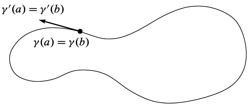
A closed curve with 
We would also like to extend the definition of the rotation index to certain piecewise regular closed curves. For this purpose, we have to take into account the “jumps” in the tangent angle function at corners. To do so, suppose ![$$\gamma :[a, b]\mathrel {\rightarrow }\mathbb {R}^2$$](../images/56724_2_En_9_Chapter/56724_2_En_9_Chapter_TeX_IEq39.png) is an admissible simple closed curve, and let
is an admissible simple closed curve, and let  be an admissible partition of [a, b]. The points
  are called the vertices of
  , and the curve segments
 ![$$\gamma |_{[a_{i-1}, a_i]}$$](../images/56724_2_En_9_Chapter/56724_2_En_9_Chapter_TeX_IEq43.png) are called its edges or sides.
are called its edges or sides.
 , recall that
  has left-hand and right-hand velocity vectors denoted by
  and
and  , respectively; let
  and
and  denote the corresponding unit vectors. We classify each vertex into one of three categories:
If
 , then
  is an ordinary vertex.
If
 , then
  is a flat vertex.
If
 , then
  is a cusp vertex.
 to be the oriented measure
  of the angle from
  to
to  , chosen to be in the interval
  , with a positive sign if
  is an oriented basis for
  , and a negative sign otherwise (Fig. 9.2). At a flat vertex, the exterior angle is defined to be zero. At a cusp vertex, there is no simple way to choose unambiguously between
  and
and  (Fig. 9.3), so we leave the exterior angle undefined. The vertex
  is handled in the same way, with T(b) and T(a) playing the roles of
  and
and  , respectively. If
  is an ordinary or a flat vertex, the interior angle at
  is defined to be
  ; our conventions ensure that
  .
.
An exterior angle
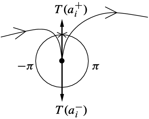
A cusp vertex
The curves we wish to consider are of the following type: a curved polygon in the plane is an admissible simple closed curve without cusp vertices, whose image is the boundary of a precompact open set  . The set
  is called the interior of
  (not to be confused with the topological interior of its image as a subset of
  , which is the empty set).
Suppose ![$$\gamma :[a, b]\mathrel {\rightarrow }\mathbb {R}^2$$](../images/56724_2_En_9_Chapter/56724_2_En_9_Chapter_TeX_IEq76.png) is a curved polygon. If
is a curved polygon. If  is parametrized so that at smooth points,
  is positively oriented with respect to the induced orientation on
  in the sense of Stokes’s theorem, we say that
  is positively oriented (Fig. 9.4). Intuitively, this means that
  is parametrized in the counterclockwise direction, or that
  is always to the left of
  .
.
 to be a piecewise continuous function
 ![$$\theta :[a, b]\mathrel {\rightarrow }\mathbb {R}$$](../images/56724_2_En_9_Chapter/56724_2_En_9_Chapter_TeX_IEq85.png) that satisfies
that satisfies  at each point t where
  is smooth, that is continuous from the right at each
  with
with
A positively oriented curved polygon


 is the exterior angle at
  . (See Figs. 9.5 and 9.6.) Such a function always exists: start by defining
  for
for  to be any lift of T on that interval; then on
  define
  to be the unique lift that satisfies (9.1), and continue by induction, ending with
  defined by (9.2). Once again, the difference between any two such functions is a constant integral multiple of
  . We define the rotation index of
  to be
to be  just as in the smooth case. As before,
  is an integer, because the definition ensures that
  .
.
Tangent angle at a vertex

Tangent angle function
The following theorem was first proved by Heinz Hopf in 1935. (For a readable version of Hopf’s proof, see [Hop89, p. 42].) It is frequently referred to by the German name given to it by Hopf, the Umlaufsatz .
Theorem 9.1
(Rotation Index Theorem). The rotation index of a positively oriented curved polygon in the plane is  .
.
Proof.
Let ![$$\gamma :[a, b]\mathrel {\rightarrow }\mathbb {R}^2$$](../images/56724_2_En_9_Chapter/56724_2_En_9_Chapter_TeX_IEq102.png) be such a curved polygon. Assume first that all the vertices of
be such a curved polygon. Assume first that all the vertices of  are flat. This means, in particular, that
  is continuous and
  . Since
  , we can extend
  to a continuous map from
  to
to  by requiring it to be periodic of period
  , and our hypothesis
  guarantees that the extended map still has continuous first derivatives. Define
  as before.
 be any lift of
  . Then
 ![$$\theta |_{[a, b]}$$](../images/56724_2_En_9_Chapter/56724_2_En_9_Chapter_TeX_IEq115.png) is a tangent angle function for
is a tangent angle function for  , and thus
  . If we set
  , then
 is also a lift of T. Because
  , it follows that
  , or in other words the following equation holds for all
  :
:
 is an arbitrary point in [a, b] and
  , then
 ![$$\gamma |_{[a_1,b_1]}$$](../images/56724_2_En_9_Chapter/56724_2_En_9_Chapter_TeX_IEq125.png) is also a positively oriented curved polygon with only flat vertices, and
is also a positively oriented curved polygon with only flat vertices, and ![$$\theta |_{[a_1,b_1]}$$](../images/56724_2_En_9_Chapter/56724_2_En_9_Chapter_TeX_IEq126.png) is a tangent angle function for it. Note that (9.3) implies
is a tangent angle function for it. Note that (9.3) implies
![$$\gamma |_{[a_1,b_1]}$$](../images/56724_2_En_9_Chapter/56724_2_En_9_Chapter_TeX_IEq127.png) has the same rotation index as
has the same rotation index as ![$$\gamma |_{[a, b]}$$](../images/56724_2_En_9_Chapter/56724_2_En_9_Chapter_TeX_IEq128.png) . Thus we obtain the same result by restricting
. Thus we obtain the same result by restricting  to any closed interval of length
  .
. achieves its minimum at
  . Moreover, by a translation in the xy-plane (which does not change
  or
or  ), we may as well assume that
  is the origin. With these adjustments, the image of
  remains in the closed upper half-plane, and
  (Fig. 9.7). By adding a constant integral multiple of
  to
to  if necessary, we can also assume that
  .
.
The curve  after changing the parameter interval and translating
  to the origin
 , representing the angle between the positive x-direction and the vector from
  to
to  . To be precise, let
  be the triangular region
  (Fig. 9.8), and define a map
  by
by
 and
and  , because
  is continuous and injective there. To see that it is continuous elsewhere, note that for
  , the fundamental theorem of calculus gives

 is uniformly continuous on the compact set [a, b], this last expression can be made as small as desired by taking
  close to (t, t). It follows that

The domain of 

The secant angle function


 to be periodic of period
  . The argument above gives
Since  is simply connected, Corollary A.57 guarantees that
  has a continuous lift
  , which is unique if we require
  (Fig. 9.9). This is our secant angle function.

 where
where  and
and ![$$t_2\in [a, b]$$](../images/56724_2_En_9_Chapter/56724_2_En_9_Chapter_TeX_IEq164.png) , the vector
, the vector  has its tail at the origin and its head in the upper half-plane. Since we stipulate that
  , we must have
 ![$$\varphi (a, t_2) \in [0,\pi ]$$](../images/56724_2_En_9_Chapter/56724_2_En_9_Chapter_TeX_IEq167.png) on this segment. By continuity, therefore,
on this segment. By continuity, therefore,  (since
  represents the tangent angle of
  ). Similarly, on the side where
  , the vector
  has its head at the origin and its tail in the upper half-plane, so
 ![$$\varphi (t_1,b)\in [\pi , 2\pi ]$$](../images/56724_2_En_9_Chapter/56724_2_En_9_Chapter_TeX_IEq173.png) . Therefore, since
. Therefore, since  represents the tangent angle of
  , we must have
  and therefore
  . This completes the proof for the case in which
  is continuous.
Now suppose  has one or more ordinary vertices. It suffices to show there is a curve with a continuous velocity vector field that has the same rotation index as
  . We will construct such a curve by “rounding the corners” of
  . It will simplify the proof somewhat if we choose the parameter interval [a, b] so that
  is not one of the ordinary vertices.
Let  be any ordinary vertex, let
  be its exterior angle, and let
  be a positive number less than
  . Recall that
  is continuous from the right at
  and
and  . Therefore, we can choose
  small enough that
  when
when  , and
, and  when
when  .
.
 of
of  is a compact set that does not contain
  , so we can choose r small enough that
  does not enter
  except when
  . Let
. Let  denote a time when
  enters
  , and
, and  a time when it leaves (Fig. 9.10). By our choice of
  , the total change in
  is not more than
  when
when  , and again not more than
  when
when ![$$t\in (a_i, t_2]$$](../images/56724_2_En_9_Chapter/56724_2_En_9_Chapter_TeX_IEq210.png) . Therefore, the total change
. Therefore, the total change  in
in  during the time interval
 ![$$[t_1,t_2]$$](../images/56724_2_En_9_Chapter/56724_2_En_9_Chapter_TeX_IEq213.png) is between
is between  and
and  , which implies
  .
.
Isolating the change in the tangent angle at a vertex

Rounding a corner
Now we simply replace ![$$\gamma |_{[t_1,t_2]}$$](../images/56724_2_En_9_Chapter/56724_2_En_9_Chapter_TeX_IEq217.png) with a smooth curve segment
with a smooth curve segment  that has the same velocity as
  at
at  and
and  , and whose tangent angle increases or decreases monotonically from
  to
to  ; an arc of a hyperbola will do (Fig. 9.11). Since the change in tangent angle of
  is between
  and
and  and represents the angle between
  and
and  , it must be exactly
  . Repeating this process for each vertex, we obtain a new curved polygon with a continuous velocity vector field whose rotation index is the same as that of
  , thus proving the theorem.
From the rotation index theorem, it is not hard to deduce the three local-to-global theorems mentioned at the beginning of the chapter as corollaries. (The angle-sum theorem is immediate; for the total curvature theorem, the trick is to show that  is equal to the signed curvature of
  ; the circumference theorem follows from the total curvature theorem as mentioned in Chapter 1.) However, instead of proving them directly, we will prove a general formula, called the Gauss–Bonnet formula, from which these results and more follow easily. You will easily see how the statement and proof of Theorem 9.3 below can be simplified in case the metric is Euclidean.
The Gauss–Bonnet Formula
![$$\gamma :[a, b]\mathrel {\rightarrow }M$$](../images/56724_2_En_9_Chapter/56724_2_En_9_Chapter_TeX_IEq234.png) is called a curved polygon in
is called a curved polygon in  if the image of
  is the boundary of a precompact open set
  , and there is an oriented smooth coordinate disk containing
  under whose image
  is a curved polygon in the plane (Fig. 9.12). As in the planar case, we call
  the interior of
  . A curved polygon whose edges are all geodesic segments is called a geodesic polygon.
A curved polygon on a surface
 in M, our previous definitions go through almost unchanged. We say that
  is positively oriented if it is parametrized in the direction of its Stokes orientation as the boundary of
  . On each smooth segment of
  , we define the unit tangent vector field
  . If
. If  is an ordinary or flat vertex, we define the exterior angle of
  at
at  as the oriented measure
  of the angle from
  to
to  with respect to the g-inner product and the given orientation of M; explicitly, this is
 at
at  is
is  . Exterior and interior angles at
  are defined similarly.
We need a version of the rotation index theorem for curved polygons in M. Suppose ![$$\gamma :[a, b]\mathrel {\rightarrow }M$$](../images/56724_2_En_9_Chapter/56724_2_En_9_Chapter_TeX_IEq257.png) is a curved polygon and
is a curved polygon and  is its interior, and let
  be an oriented smooth chart such that U contains
  . Using the coordinate map
  to transfer
  ,
,  , and g to the plane, we may as well assume that g is a metric on some open subset
  , and
, and  is a curved polygon in
  . Let
. Let  be the oriented orthonormal frame for g obtained by applying the Gram–Schmidt algorithm to
  , so that
  is a positive scalar multiple of
  everywhere in
  .
.
 to be a piecewise continuous function
 ![$$\theta :[a, b]\mathrel {\rightarrow }\mathbb {R}$$](../images/56724_2_En_9_Chapter/56724_2_En_9_Chapter_TeX_IEq273.png) that satisfies
that satisfies
 is continuous, and that is continuous from the right and satisfies (9.1) and (9.2) at vertices. The existence of such a function follows as in the planar case, using the fact that
![$$u_1,u_2:[a, b]\mathrel {\rightarrow }\mathbb {R}$$](../images/56724_2_En_9_Chapter/56724_2_En_9_Chapter_TeX_IEq275.png) that can be regarded as the coordinate functions of a map
that can be regarded as the coordinate functions of a map ![$$(u_1,u_2):[a, b]\mathrel {\rightarrow }\mathbb S^1$$](../images/56724_2_En_9_Chapter/56724_2_En_9_Chapter_TeX_IEq276.png) because T has unit length.
because T has unit length.The rotation index of  is
is  . Because of the role played by the specific frame
  in the definition, it is not obvious that the rotation index has any coordinate-independent meaning; however, the following easy consequence of the rotation index theorem shows that it does not depend on the choice of coordinates.
Lemma 9.2.
If M is an oriented Riemannian 2-manifold, the rotation index of every positively oriented curved polygon in M is  .
.
Proof.
If we use the given oriented coordinate chart to regard  as a curved polygon in the plane, we can compute its tangent angle function either with respect to g or with respect to the Euclidean metric
  . In either case,
  is an integer because
  and
and  both represent the angle between the same two vectors, calculated with respect to some inner product. Now for
  , let
, let  . By the same reasoning, the rotation index
  with respect to
  is also an integer for each s, so the function
  is integer-valued.
In fact, the function f is continuous in s, as can be deduced easily from the following observations: (1) Our preferred  -orthonormal frame
  depends continuously on s, as can be seen from the formulas (2.5)–(2.6) used to implement the Gram–Schmidt algorithm. (2) On every interval
 ![$$[a_{i-1}, a_i]$$](../images/56724_2_En_9_Chapter/56724_2_En_9_Chapter_TeX_IEq293.png) where
where  is smooth, the functions
  and
and  satisfying the
  -analogue of (9.5) can be expressed as
  , where
  . Thus
  and
and  depend continuously on
 ![$$(t, s)\in [a_{i-1}, a_i]\times [0,1]$$](../images/56724_2_En_9_Chapter/56724_2_En_9_Chapter_TeX_IEq302.png) , so the function
, so the function ![$$(u_1,u_2):[a_{i-1}, a_i]\times [0,1]\mathrel {\rightarrow }\mathbb S^1$$](../images/56724_2_En_9_Chapter/56724_2_En_9_Chapter_TeX_IEq303.png) has a continuous lift
has a continuous lift ![$$\theta :[a_{i-1}, a_i]\times [0,1]\mathrel {\rightarrow }\mathbb {R}$$](../images/56724_2_En_9_Chapter/56724_2_En_9_Chapter_TeX_IEq304.png) , uniquely determined by its value at one point. (3) At each vertex, it follows from formula (9.4) that the exterior angle depends continuously on
, uniquely determined by its value at one point. (3) At each vertex, it follows from formula (9.4) that the exterior angle depends continuously on  .
.
Because f is continuous and integer-valued, it follows that  , which was to be proved.
 is given a unit-speed parametrization, so the unit tangent vector field T(t) is equal to
  . There is a unique unit normal vector field N along the smooth portions of
  such that
  is an oriented orthonormal basis for
  for each t. If
  is positively oriented as the boundary of
  , this is equivalent to N being the inward-pointing normal to
  (Fig. 9.13). We define the signed curvature of
  at smooth points of
  by
by

 , we see that
  is orthogonal to
  , and therefore we can write
  , and the (unsigned) geodesic curvature of
  is
is  . The sign of
  is positive if
  is curving toward
  , and negative if it is curving away.
N(t) is the inward-pointing normal
Theorem 9.3
 is a positively oriented curved polygon in M, and
  is its interior. Then
 are the exterior angles of
  , and the second integral is taken with respect to arc length (Problem 2-32).
Proof.
 be an admissible partition of [a, b], and let (x, y) be oriented smooth coordinates on an open set U containing
  . Let
. Let ![$$\theta :[a, b]\mathrel {\rightarrow }\mathbb {R}$$](../images/56724_2_En_9_Chapter/56724_2_En_9_Chapter_TeX_IEq334.png) be a tangent angle function for
be a tangent angle function for  . Using the rotation index theorem and the fundamental theorem of calculus, we can write
 ,
,  , and K.
 be the oriented g-orthonormal frame obtained by applying the Gram–Schmidt algorithm to
  as before. Then by definition of
  and N, the following formulas hold at smooth points of
  :
:
 (and omitting the t dependence from the notation for simplicity), we get
 and
and  . Because
  is an orthonormal frame, for every vector v we have
 is a multiple of
  and
and  is a multiple of
  . Define a 1-form
  by
by

 completely determines the connection in U. (In fact, when the connection is expressed in terms of the local frame
  as in Problem 4-14, this computation shows that the connection 1-forms are just
  ,
,  ; but it is simpler in this case just to derive the result directly as we have done.)


 is a smooth manifold with corners (see [LeeSM, pp. 415–419]), we can apply Stokes’s theorem and conclude that the left-hand side of (9.10) is equal to
  . The last step of the proof is to show that
  . This follows from the general formula relating the curvature tensor and the connection 1-forms given in Problem 7-5; but in the case of two dimensions we can give an easy direct proof. Since
  is an oriented orthonormal frame, it follows from Proposition 2.41 that
  . Using (9.9), we compute
![$$\begin{aligned} \begin{aligned} K\, dA(E_1,E_2)&= K = Rm(E_1,E_2,E_2,E_1)\\&= \left\langle \nabla _{E_1} \nabla _{E_2} E_2 - \nabla _{E_2} \nabla _{E_1} E_2 - \nabla _{[E_1,E_2]} E_2 ,\ E_1\right\rangle \\&= \left\langle \nabla _{E_1} (\omega (E_2) E_1 ) - \nabla _{E_2} (\omega (E_1) E_1) - \omega ([E_1,E_2]) E_1,\ E_1\right\rangle \\&= \left\langle E_1 (\omega (E_2)) E_1 + \omega (E_2)\nabla _{E_1} E_1 - E_2(\omega (E_1)) E_1\right. \\&\qquad - \left. \omega (E_1) \nabla _{E_2} E_1 - \omega ([E_1,E_2]) E_1,\ E_1\right\rangle \\&= E_1 (\omega (E_2)) - E_2(\omega (E_1)) - \omega ([E_1,E_2]) \\&= d\omega (E_1,E_2). \end{aligned} \end{aligned}$$](../images/56724_2_En_9_Chapter/56724_2_En_9_Chapter_TeX_Equ33.png)

The three local-to-global theorems of plane geometry stated in Chapter 1 follow from the Gauss–Bonnet formula as easy corollaries.
Corollary 9.4
(Angle-Sum Theorem). The sum of the interior angles of a Euclidean triangle is  .
. 
Corollary 9.5
(Circumference Theorem). The circumference of a Euclidean circle of radius R is  .
. 
Corollary 9.6
![$$\gamma :[a, b]\mathrel {\rightarrow }\mathbb {R}^2$$](../images/56724_2_En_9_Chapter/56724_2_En_9_Chapter_TeX_IEq365.png) is a smooth, unit-speed, simple closed curve such that
is a smooth, unit-speed, simple closed curve such that  , and N is the inward-pointing normal, then

The Gauss–Bonnet Theorem
It is now a relatively easy matter to “globalize” the Gauss–Bonnet formula to obtain the Gauss–Bonnet theorem. The link between the local and global results is provided by triangulations, so we begin by discussing this construction borrowed from algebraic topology.
 is a curved polygon with exactly three edges and three vertices. A smooth triangulation of
  is a finite collection of curved triangles with disjoint interiors such that the union of the triangles with their interiors is M, and the intersection of any pair of triangles (if not empty) is either a single vertex of each or a single edge of each (Fig. 9.14). Every smooth, compact surface possesses a smooth triangulation. In fact, it was proved by Tibor Radó [Rad25] in 1925 that every compact topological 2-manifold possesses a triangulation (without the assumption of smoothness of the edges, of course), in which every edge belongs to exactly two triangles. There is a proof for the smooth case that is not terribly hard, based on choosing geodesic triangles contained in convex geodesic balls (see Problem 9-5).
Valid and invalid intersections of triangles in a triangulation
 (with respect to the given triangulation) is defined to be

Theorem 9.7

Proof.
We may as well assume that M is connected, because if not we can prove the theorem for each connected component and add up the results.
 gives the same result whether we interpret dA as the Riemannian density or as the Riemannian volume form, so we will use the latter interpretation for the proof. Let
  denote the faces of the triangulation, and for each i, let
  be the edges of
  and
and  its interior angles. Since each exterior angle is
  minus the corresponding interior angle, applying the Gauss–Bonnet formula to each triangle and summing over i gives
 all cancel out. Thus (9.11) becomes
 appears exactly once. At each vertex, the angles that touch that vertex must have interior measures that add up to
  (Fig. 9.15); thus the angle sum can be rearranged to give exactly
  . Equation (9.12) thus can be written

Interior angles at a vertex add up to 
 , where we count each edge once for each triangle in which it appears. This means that
  , so (9.13) finally becomes
![$${\smash [t]{\widehat{M}}}$$](../images/56724_2_En_9_Chapter/56724_2_En_9_Chapter_TeX_IEq385.png) that admits a 2-sheeted smooth covering
that admits a 2-sheeted smooth covering ![$$\hat{\pi }:{\smash [t]{\widehat{M}}}\mathrel {\rightarrow }M$$](../images/56724_2_En_9_Chapter/56724_2_En_9_Chapter_TeX_IEq386.png) , and Exercise A.62 shows that
, and Exercise A.62 shows that ![$${\smash [t]{\widehat{M}}}$$](../images/56724_2_En_9_Chapter/56724_2_En_9_Chapter_TeX_IEq387.png) is compact. If we endow
is compact. If we endow ![$${\smash [t]{\widehat{M}}}$$](../images/56724_2_En_9_Chapter/56724_2_En_9_Chapter_TeX_IEq388.png) with the metric
with the metric  , then the Riemannian density of
  is given by
  , and its Gaussian curvature is
  , so
, so  . The result of Problem 2-14 shows that
 ![$$\int _{{\smash [t]{\widehat{M}}}} \hat{K}\,\widehat{dA} = 2\int _M K\, dA$$](../images/56724_2_En_9_Chapter/56724_2_En_9_Chapter_TeX_IEq394.png) .
.To compare Euler characteristics, we will show that the given triangulation of M “lifts" to a smooth triangulation of ![$${\smash [t]{\widehat{M}}}$$](../images/56724_2_En_9_Chapter/56724_2_En_9_Chapter_TeX_IEq395.png) . To see this, let
. To see this, let  be any curved triangle in M and let
  be its interior. By definition, this means that there exists a smooth chart
  whose domain contains
  and whose image is a disk
  , and such that
  , where
  is the interior of a curved triangle
  in
in  . Then
  is an embedding of D into M, which restricts to a diffeomorphism
  . Because D is simply connected, it follows from Corollary A.57 that
  (and therefore also F) has a lift to
 ![$${\smash [t]{\widehat{M}}}$$](../images/56724_2_En_9_Chapter/56724_2_En_9_Chapter_TeX_IEq408.png) , which is smooth because
, which is smooth because  is a local diffeomorphism; and because the covering is two-sheeted, there are exactly two such lifts
  . Each lift is injective because
  , which is injective, and their images are disjoint because if two lifts agree at a point, they must be identical. From this it is straightforward to verify that the lifted curved triangles form a triangulation of
 ![$${\smash [t]{\widehat{M}}}$$](../images/56724_2_En_9_Chapter/56724_2_En_9_Chapter_TeX_IEq412.png) with twice as many vertices, edges, and faces as that of M, and thus
with twice as many vertices, edges, and faces as that of M, and thus ![$$\chi \bigl ({\smash [t]{\widehat{M}}}\bigr ) = 2\chi (M)$$](../images/56724_2_En_9_Chapter/56724_2_En_9_Chapter_TeX_IEq413.png) . Substituting these relations into the Gauss–Bonnet theorem for
. Substituting these relations into the Gauss–Bonnet theorem for ![$${\smash [t]{\widehat{M}}}$$](../images/56724_2_En_9_Chapter/56724_2_En_9_Chapter_TeX_IEq414.png) and dividing through by 2, we obtain the analogous relation for M.
and dividing through by 2, we obtain the analogous relation for M. 
The significance of this theorem cannot be overstated. Together with the classification theorem for compact surfaces, it gives us very detailed information about the possible Gaussian curvatures for metrics on compact surfaces. The classification theorem [LeeTM, Thms. 6.15 and 10.22] says that every compact, connected, orientable 2-manifold M is homeomorphic to a sphere or a connected sum of n tori, and every nonorientable one is homeomorphic to a connected sum of n copies of the real projective plane  ; the number n is called the genus of
  . (The sphere is said to have genus zero.) By constructing simple triangulations, one can show that the Euler characteristic of an orientable surface of genus n is
  , and that of a nonorientable one is
  . The following corollary follows immediately from the Gauss–Bonnet theorem.
Corollary 9.8
Let (M, g) be a compact Riemannian 2-manifold and let K be its Gaussian curvature.
- (a)
If M is homeomorphic to the sphere or the projective plane, then
 somewhere.
 - (b)
If M is homeomorphic to the torus or the Klein bottle, then either
 or K takes on both positive and negative values.
 - (c)
If M is any other compact surface, then
 somewhere.
This corollary has a remarkable converse, proved in the mid-1970s by Jerry Kazdan and Frank Warner: If K is any smooth function on a compact 2-manifold M satisfying the necessary sign condition of Corollary 9.8, then there exists a Riemannian metric on M for which K is the Gaussian curvature. The proof is a deep application of the theory of nonlinear partial differential equations. (See [Kaz85] for a nice expository account.)
In Corollary 9.8 we assumed we knew the topology of M and drew conclusions about the possible curvatures it could support. In the following corollary we reverse our point of view, and use assumptions about the curvature to draw conclusions about the topology of the manifold.
Corollary 9.9
Let (M, g) be a compact Riemannian 2-manifold and K its Gaussian curvature.
- (a)
If
 everywhere on M, then the universal covering manifold of M is homeomorphic to
  , and
, and  is either trivial or isomorphic to the two-element group
  .
. - (b)
If
 everywhere on M, then the universal covering manifold of M is homeomorphic to
  , and
, and  is infinite.
Proof.
Suppose first that M has positive Gaussian curvature. From the Gauss–Bonnet theorem, M has positive Euler characteristic. The classification theorem for compact surfaces shows that the only such surfaces are the sphere (with trivial fundamental group) and the projective plane (with fundamental group isomorphic to  ), both of which are covered by the sphere.
On the other hand, suppose M has nonpositive Gaussian curvature. Then its Euler characteristic is nonpositive, so it is either an orientable surface of genus  or a nonorientable one of genus
  . Thus the universal covering space of M is
  if M is the torus or the Klein bottle, and
  in all other cases (see [LeeTM, Thm. 12.29]), both of which are homeomorphic to
  . The fact that the universal covering space is noncompact implies that the universal covering map has infinitely many sheets by the result of Exercise A.62, and then Proposition A.61 shows that
  is infinite.
Much of the effort in contemporary Riemannian geometry is aimed at generalizing the Gauss–Bonnet theorem and its topological consequences to higher dimensions. As we will see in the next few chapters, most of the interesting results have required the development of different methods.
However, there is one rather direct generalization of the Gauss–Bonnet theorem that deserves mention. For a compact manifold M of any dimension, the Euler characteristic of  , denoted by
  , can be defined analogously to that of a surface and is a topological invariant (see [LeeTM, Thm. 13.36]). It turns out that it is always zero for an odd-dimensional compact manifold, but it is a nontrivial invariant in each even-dimensional case.


