Economics Demystified®

chapter 1

Introduction to Economics

This chapter introduces what economics is and why people are sometimes confused by the subject. In addition to the jargon that economists use, economics requires a different way of thinking about problems from the way most people are used to. While economists disagree on many topics, there are some basic principles that they do agree on.

CHAPTER OBJECTIVES

After completing this chapter, the student should be able to:

1. Describe the reasons why many people struggle with economics.

2. Describe what is meant by economic resources.

3. Define opportunity costs and explain why opportunity costs are considered more important than explicit costs.

4. Describe what is meant when economists say that someone thinks “rationally.”

5. Define microeconomics and macroeconomics and be able to describe the difference between them.

As two self-described “econ-nerds,” your coauthors have each, more times than we care to admit, engaged in versions of the following conversation:

New person (NP): “So what do you do?”

EN (politely, but vaguely): “I’m a college professor.”

NP (sensing a productive and perhaps interesting conversation): “Oh really? What do you teach?”

EN (sensing where this is heading): “Economics.”

NP (awkward pause, followed by one of the following):

a. “Wow! I hated that class in college!”

b. “Really? Where do you think the stock market is headed?”

c. “Now there’s something that I’ll never understand.”

EN (a little sheepishly): “Yes, I hear that a lot. Did you try that cheese platter? It’s amazing!”

So why do so many people we meet have such adverse reactions to the topic? And why are these people so ready to share with us the reasons why they hate economics? We think there are three main factors:

1. Language barriers. Economists have unintentionally made their social interactions more difficult because they use complicated language to communicate simple ideas. Economists have managed to make common sense as difficult as possible. People read the headlines on “double-dip recession” or “currency revaluation” and just don’t want to read any further. And who can blame them? In the interest of demystifying economics for you, we define some of these key words and phrases in a way that we think translates the complex language of economists into something simpler and more understandable.

2. Economists don’t always agree. People often hear two economists making very different predictions about the same topic. One economist says that universal health care will reduce the federal budget deficit, while another states, with equal confidence, that universal health care will add to the deficit. This is very frustrating to people who genuinely want to be informed about such things. This frustration causes many people to tune out the debate and conclude that economists really don’t know what they’re talking about.

How can it be that these two “experts” can make such conflicting predictions? The explanation lies in the way in which economists do their research. Economists use theoretical models, simplified versions of the complex world, to predict how changes in one thing will affect other things. Underlying these economic models are assumptions concerning the way the world works. For example, the first economist believes that even if it increases the size of government, universal health care will push the price of medical services downward, making it less expensive for even a larger government to insure people and thus reducing the deficit. The second economist believes that, while the first argument might have some merit, the increased size and cost of the government bureaucracy will outweigh the cost savings for medical services. For the most part, the public wants easy answers to policy questions like the impact of universal health care, but the world is a very complicated place. The economists try to inform these debates with their best economic models, and different assumptions will often produce different predictions. When we look at some of these models, we try to demystify how critical some of these assumptions can be.

3. Math is involved (and graphs, but those are really just math in picture form). The state of Kentucky, like many states faced with a budget deficit, recently increased the tax on tobacco products. Most people understand that a higher tax on tobacco will increase the price of cigarettes to the consumer, and that fewer cartons of cigarettes will be purchased at the higher price. But economists ask a very important question that can be answered only with a little bit of math: “If the price of cigarettes is rising and fewer cigarettes are being bought, will the government actually receive more or less tax revenue from cigarette sales?” While much of the economic research out there involves some high-level math, we believe that most of economics can be demystified with just a few simple mathematical techniques and graphical analysis. The appendix to this chapter provides a little review if you think it’s necessary.

Before we get into the real guts of the economic language, models, and graphical analysis, let’s cover just a few of the basics that all economists can agree upon, starting with how economics is divided. When the focus is on the decisions made by individuals, households, firms, or industries, we are referring to the subfield of microeconomics. When the focus is on the decisions made by nations, we are referring to macroeconomics.

Scarcity

There is no fundamental economic concept that enjoys as much universal support from economists as does the concept of scarcity. Scarcity is the unfortunate imbalance between our limitless wants and needs and the limited resources that are available to satisfy those wants and needs. Scarcity is really very simple, but it drives all of our decision making and our behavior, and it forces us to choose some goods at the expense of other goods. For example, if a consumer chooses to purchase a $4 gallon of gasoline with her limited income, she cannot use that $4 to consume something else. If a nation chooses to spend $4 billion to improve the highway system, that $4 billion cannot be spent on education. The field of economics studies how society, whether it is the single consumer or a nation, can best make those decisions when confronted with scarcity.

Four Economic Resources

A key component of the notion of scarcity is the fact that society’s enjoyment of goods and services is limited by the resources available to us. Economists typically recognize four categories of resources that are available to produce the items that we want.

1. Labor (usually abbreviated as L). The collective size and effort of a nation’s workforce.

2. Capital (K). The manufactured productive assets (buildings, tools, and machinery) in the nation.

3. Land (or natural resources, l). The nation’s stock of minerals, timber, fisheries, water, and so on.

4. Entrepreneurship (or technology, A). The nation’s ability to creatively combine the labor, capital, and land to produce goods and services.

Still Struggling

Some students may be confused by the fact that the one “resource” they think is most associated with economics is not here: money. That is because money is not a resource. In economics, a resource is something that is used to create other things of value. For instance, a house is made by combining labor for the construction workers, capital in the form of equipment used to build the house, land in the form of the lumber and energy used, and entrepreneurship in the form of the “know-how” required to put the house together. Money isn’t actually used to build the house; it just facilitates the exchange of all these things.

When you hear nerdy economists talk about resources, they are referring to those listed earlier. However, we often hear noneconomists talk about a firm that needs to “find additional resources” or “raise more capital.” We believe that these statements are inaccurate, because the people making them are usually referring to the firm’s need for more cash or other forms of money. Cash and other forms of money are not resources. They simply make it easier to obtain the needed resources. For example, suppose an entrepreneur wants to produce tables and sell those tables at his furniture store. He will certainly need cash to begin this company, but the cash is simply used to purchase the economic resources (labor, capital, and natural resources) that will actually be involved in the production of tables.

Opportunity Cost

Scarcity requires us to make choices. A consumer who chooses to purchase gasoline rather than a new pair of running shoes has given up the enjoyment that she would have received from the new shoes. Economists refer to this sacrifice as the opportunity cost. The opportunity cost of a choice, like the gasoline, is measured as the value of the next best thing the consumer has given up. How do we place a value on the enjoyment that the running shoes would have provided to our consumer? Economists believe that the price of a product, in this case the shoes, provides a pretty good idea of how much value consumers place upon it. After all, if people are paying $100 for a pair of running shoes, they must believe that they will receive at least $100 worth of enjoyment from them.

Here is where economists tend to think a little differently from “normal people.” To an economist, the opportunity cost is more important than the cost measured in dollar terms. Why? Well, opportunity costs reflect what the true cost of something is. Consider the dollar price of something (also called an explicit price) like a concert ticket. If it is for an extremely popular band, chances are that you are going to have to wait in line to ensure that you get a ticket. So even if the face value of the ticket is only $80, the other costs involved may be substantial and may even outweigh the dollar price of the ticket. The true cost of the ticket was all the other things you could have purchased with the $80 plus the opportunity cost of the time involved in purchasing the ticket.

Rational Decision Making

Let’s return to the example of the consumer who buys gasoline instead of running shoes. Why did she do this? An economist believes that she has examined her choices and, within the limits of her budget, has made a rational decision to forgo the shoes and purchase the gasoline because doing so makes her better off. Specifically, we assume that the rational consumer goes through life making decisions that will maximize her utility (the word that economists use to describe happiness, usefulness, or economic benefit). Rational consumers seek those things that make them the most happy (provide the most benefit) and avoid those things that make them unhappy (incur lots of cost). In other words, we all attempt to seek economic benefit and attempt to avoid economic cost. We will develop the model of consumer choice in Chapter 2.

Does that mean that consumers always make the best decisions? Not necessarily. All agents make decisions based on the information that they have available. If that information is incomplete or flawed, they might make a decision that they think will make them better off but that in fact does not. A classic example of this is a purchase that generates pollution. When gasoline, a polluting substance, is fairly cheap, people might end up consuming “too much” because they aren’t aware of the pollution that it causes. We talk about this later in Chapter 18. What rationality does mean, however, is that decision makers do not knowingly make themselves worse off.

Marginal Analysis

If we accept the premise that consumers seek economic benefit and avoid economic cost, then we must assume that people try to maximize the difference, or net benefit, between the economic benefits they enjoy and the economic costs they incur through their decisions.

People often make decisions to consume or do something on an incremental basis, and at each step of these incremental decisions, they must reevaluate the benefits that they receive and the costs that they incur. Economists refer to the additional benefit received from the next unit of a good as the marginal benefit and the additional cost incurred from the next unit as the marginal cost.

For example, if I believe that I will enjoy $6 of economic benefit from my first cup of coffee, and that cup of coffee comes at a cost of $2, I am receiving $4 of net benefit from the coffee and it would be rational for me to purchase it. Suppose the second cup of coffee would provide me with only $4 of marginal benefit. Should I purchase the second cup? Yes, because I will still enjoy $2 of net benefit ($4 of enjoyment minus $2 of marginal cost) from the coffee. Maybe the third cup of coffee provides me with only $2 of marginal benefit. Should I buy it? Yes, because there is a perfect trade-off between $2 of marginal benefit and $2 of marginal cost. However, suppose the fourth cup of coffee makes me extremely jittery and won’t give me any marginal benefit. As a rational consumer, I will not buy the fourth cup of coffee because the marginal cost is greater than the marginal benefit. In fact, the fifth cup kind of makes me nauseous and imposes negative $2 of marginal benefit, so I clearly won’t purchase that one either.

The marginal benefits and costs from my coffee consumption are described in Table 1-1.

TABLE 1-1 Marginal Benefits and Marginal Costs of Coffee Consumption

So long as the marginal benefit of the next unit of something is at least as great as the marginal cost of that unit, the consumer should always purchase the next unit. By consuming three cups of coffee, I receive a total benefit of $6 , and thus by making my decisions “at the margin,” I have picked the quantity of coffee that maximizes my total net benefit. Had I irrationally consumed the fourth cup, my total net benefit from coffee would have fallen to $4, so I will not make this choice. We will show in several upcoming chapters the importance of marginal analysis in economic decision making.

A common approach that people use when they think about costs and benefits is to think about things “on average.” This can lead to irrational behavior. For example, consider the previous example about coffee. If I had consumed five cups of coffee, I would have enjoyed total benefit of , and so, on average, each cup provided an average benefit of $2 per cup. Given this calculation, one might be tempted to say that each cup was “worth” the price of $2 per cup. Was it? No! Drinking that fifth cup would actually have made me worse off.

Economic Models

A paper airplane is not a real airplane, but it has some of the important features of the real thing. We know that a real airplane is much more complex, but a person can see a lot about the fundamentals of aerodynamics by watching the way a paper airplane glides through the air. In the same way, economic models attempt to depict the decisions that consumers, firms, and nations make in a very complex, dynamic world. If a simple economic model can distill these complexities into something that reasonably predicts the outcome of economic decisions, it can be a powerful tool for us.

One important feature of economic models is the need to make assumptions about behavior. For example, in the model of consumer behavior in Chapter 2, we assume that consumers seek to maximize their utility within the constraints of their budget. Later in the book, we assume that firms seek to maximize their profits. Given these assumptions of behavior, we can study how choices are made to pursue the goals of utility (or profit) maximization.

Economic models can be very useful when they can predict how the change in one variable affects the decisions that consumers and firms make. The problem is that, in the real world, there are many variables that are changing at the same time. This makes it very difficult to isolate the impact of a change in just one key variable. Therefore, a second important feature of economic models is the use of the ceteris paribus, or “all other factors held constant,” condition.

For example, we might wish to study how consumers react to a higher tax on electricity. We realize that, in reality, there are many factors that affect a consumer’s decision to buy a certain amount of electricity for his household. The economist’s model will predict that an increased tax on electricity, holding all other factors (like consumer income, weather conditions, and so on) constant, should prompt consumers to purchase less electricity. In fact, it is the ceteris paribus assumption that allows us to study a fundamental economic model such as the model of demand and supply.

Summary

This chapter described some of the basic ideas of economics. Scarcity is the basis of economics, as we all have unlimited wants, but we are faced with limitations on how we can satisfy those wants. Opportunity costs are the most relevant costs to an economic thinker, because the value of the next best alternative to something is what you are really giving up to get that thing. We use resources to try to create things that will satisfy our wants, and resources can be broken down into four categories: land, labor, capital, and entrepreneurship. A major assumption that economists make about agents is that they will act rationally, meaning mainly that they tend to make decisions based on the marginal benefits and marginal costs of those decisions. The basic idea behind economics is that every agent tries to make herself as well off as possible, and economics just describes the way in which agents go about making that happen. In the next chapter, we turn our attention to exactly how one group of agents, buyers, tries to make itself as happy as possible.

Appendix
Math and Graph Review

There are two reasons that students tend to fear economics: math and graphs. The good news is that the math isn’t really all that complicated; in fact, you have almost certainly seen math just like it before. The math that is used in most introductory economics courses is no more complicated than what you did your first or second year of high school. There is a (very) little bit of algebra, an even smaller amount of geometry, and a lot of graphical analysis.

To lessen your anxiety, this appendix will walk you through the graphing and math that you are likely to encounter in an introductory economics course. The most common math you will encounter in such a course can be broken down into four categories: graphing, simple calculations, calculating area, and solving a system of two equations. Here is a tip before we continue: every graph and every equation you see, you should also be drawing and writing down. The best way to get experience using these types of analysis is to take pen to paper and practice, practice, practice.

Graphs—Pictures of Equations

A graph is simply a pictorial representation of the relationship between two things. In previous math courses, you have probably seen graphs represented on the Cartesian coordinate system. In this system, the “two things” are x and y, which are represented on the two axes (or sides) of a graph, and any lines or points on the graph show the particular value of y that goes with a particular value of x. In the case of a line, there is usually an equation that describes the relationship between x and y mathematically, and the graph simply translates that equation into a picture. Each of the axes represents a number line, and the axes intersect each other at zero.

The Cartesian coordinate system can be broken down into four quarters, I, II, III and IV, as shown in Figure 1-1. Each point on the Cartesian plane is a representation of a combination of a particular value of x and a value y associated with that value of x. For instance, in Figure 1-1, point A represents , and point E represents .

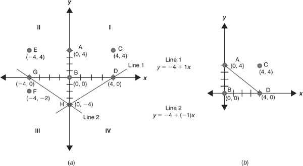
FIGURE 1-1 • (a) The Cartesian Coordinate System; (b) the Plane Typically Used in Economics. Each point represents a combination of coordinates (x, y). For the points in (a), the coordinates are , and .

Line 1 in Figure 1-1a is a pictorial representation of the equation . Given the equation of this line, we can find the values of y that correspond to different values of x. For instance, point D on Figure 1-1a corresponds to the point (4, 0). Plugging the value of x into the equation, we get . Similarly, point H corresponds to the point (0, −4), and if we plug the value of into the equation, . The line is merely the description of all the possible values of y that will correspond to any given value of x.

There are two things to note about the relationship between the equation and the graph. First, −4 in the equation for line 1 is the point at which the line crosses the y axis. Second, the slope of this line is equal to +1, meaning that every time x increases by 1 unit, the corresponding value of y will also increase by 1 unit. In general, the equation of any line in the Cartesian plane can be expressed as , where a represents the y intercept and b is the slope of the line. In our example, and . Any time that b is a positive number, the line slopes upward. On the other hand, consider line 2 in Figure 1-1a. The equation for this line is . This equation is different from line 1 only in slope—the lines representing both equations cross the y axis at the same point, but line 2 is downward-sloping, so that every increase of 1 unit in x leads to a decrease of 1 unit in y.

Here is the good news about graphs in economics: we focus almost exclusively on quadrant I, which means that we get to simplify this even further. As practice, try recreating Figure 1-1a and then 1-1b, on graph paper if it helps, using the coordinates listed beneath each. Then, check your work against the graph. Next, try to figure out the equation of the line in Figure 1-1b using the format. (We’ll give you the answer at the end of the appendix.)

Where graphs in economics differ from the graphs you’ve seen before is that we are interested in the relationship between the things that x and y represent. Suppose we conducted a survey and asked four people what they had ordered for lunch at a fast food restaurant in terms of burgers and fries. We will let x indicate how many burgers each respondent ordered and y indicate how many fries each respondent ordered, and adapt Figure 1-1b to reflect this change, as shown in Figure 1-2. Each point now corresponds with the particular combination of hamburgers and fries that a particular person ordered. Thus, person A ordered no burgers and 4 orders of fries, person C ordered 4 burgers and 4 orders of fries, and so on.

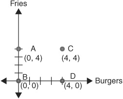
FIGURE 1-2 • Responses to a Survey on Fast Food Orders

Let’s take another example and look at the relationship between the price of a good and how much of that good people are willing to buy. Suppose that we know for certain that nobody will ever buy a particular good, purpletts, if the price of it is greater than $20. In other words, if price is our y variable, then if , . We also know that once the price dips below $20, people will buy the good. In fact, for every $1 that the price drops, people will buy 1 more purplett. So if the price of purpletts is $19, people will buy a total of 1 purplett; if the price drops to $18, people will buy a total of 2 purpletts; and so on. We could figure this out for all possible quantities using the following equation:

and so on.

In equation form, we could represent the relationship between the price of purpletts and the amount of purpletts that people buy as , where 20 is the price axis intercept and the slope of the line is . Graphically, we show this in Figure 1-3. Try creating Figure 1-3 on your own, calculating the quantities that are bought at various prices and then plotting those combinations on your graph. As you recreate Figure 1-3 on your own, notice that each value of Q corresponds with a value of P according to the demand equation. For instance, when the price of purpletts is $10 each, people are willing and able to buy 10 purpletts, which corresponds to the point (10, $10) on the curve on the graph.

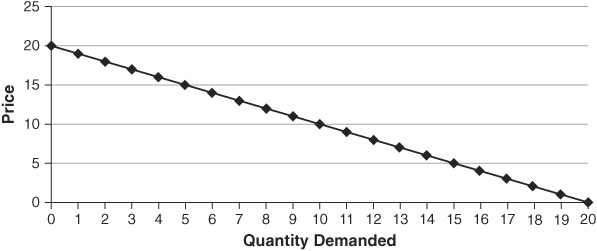
FIGURE 1-3 • Demand for Purpletts

In Chapter 3 we will learn that when any of the determinants of demand change, the demand curve shifts. A shift of a curve is a change of the intercept (a), not the slope. For instance, a shift of the demand curve to the right would mean that for any given price, more Q is demanded. Such a shift is shown in Figure 1-4. Note that on the curve Demand 1, when , people were willing and able to buy 10 units of purpletts, and when , people were willing and able to buy 0 units of purpletts. Now that demand has shifted out to Demand 2, when , people are willing and able to buy 14 units of purpletts, and when , people are willing and able to buy 4 units of purpletts. This new demand curve is consistent with an equation .

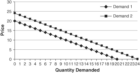
FIGURE 1-4 • Shifting Demand for Purpletts

Of course, you can also have relationships that are nonlinear, that is, that are not straight lines. A common nonlinear function (that is, the equation that represents a curve) that you see in economics is binomial. These types of functions typically take the form . These functions are often called quadratic functions and will have either a “U” shape or a “hill” shape.

For example, suppose that corn production (y) is a binomial function of rainfall (x) such that . (Note: We might model corn production this way because, in agriculture, there can be both insufficient rain and too much rain.) Figure 1-5 shows how this function would look in a graph. Notice that at first, more rain causes corn production to “grow,” but the additional rain has a smaller and smaller impact on the harvest. In fact, at , corn production is as great as it can be. If the crops get even more rain, output will actually begin to decline, and eventually the entire crop will be wiped out.

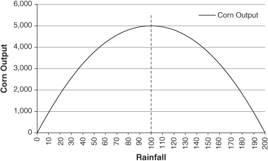
FIGURE 1-5 • Corn Output as a Function of Rainfall

Unlike a straight line, which has a constant slope, these binomial functions have a slope that varies. The corn production function begins with a positive slope (more rain = more corn), but that slope begins to become less and less positive; the function is increasing at a decreasing rate. When we reach the maximum of the function, the slope is equal to zero. Beyond the maximum point, the function has a negative slope, and as rainfall increases, that slope becomes even more negative; the function is decreasing at an increasing rate.

Economists also study binomial functions that have a U shape (think of this as the hill shape, just upside down). Average total cost (ATC) curves are typically described this way. Let’s suppose that average total cost (y) is a function of a firm’s output (x) such that . This ATC function is shown in Figure 1-6. We see that, at first, additional output causes ATC to decline, but at 10 units of output, the ATC is minimized. Beyond 10 units of output, ATC is rising. We discuss cost curves in much more detail in Chapter 4 of the book.

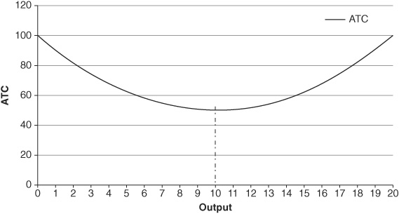
FIGURE 1-6 • Average Total Cost as a Function of Output

Again, the slope of this function is not constant. At first the slope is negative and steep, but as output increases, the slope becomes less steep; the function is decreasing at a decreasing rate. The slope is zero at the minimum point, and from that point forward, the slope is positive and is becoming steeper; the function is increasing at an increasing rate.

Simple Math: Calculating Percentages

Economists are frequently interested in the relative change in something rather than the actual amount of the change. For instance, suppose Eli gets an increase of $10 in his weekly allowance and Max gets an increase of $5 in his weekly allowance. Eli got the better increase . . . or did he? We actually can’t tell who was made better off than he was previously without knowing what their allowances were before. Suppose that, prior to the increase, Eli got an allowance of $40 a week and Max got an allowance of $4. Max’s allowance has more than doubled, meaning that Max can buy more than twice as much stuff as he could before, but Eli’s didn’t double, so he can’t buy twice as much as he could before. Max’s “raise” was clearly better in terms of the magnitude of the change.

An easy way to control for relative differences is to compute a percentage. Doing so is actually fairly simple and most easily illustrated with an example. Suppose you have a box of 50 chocolates, and 7 of them have nougat filling inside. You are interested in the percentage of nougat-filled chocolates in a box. To find this you divide the value of the part you are interested by the value of the whole and multiply that number by 100 to get the percentage. In this case:

Therefore, the box of chocolates is 14 percent nougat-filled. Note that we can rearrange this to get a different type of problem. Suppose we solved instead for “Part” by rearranging Eq. (1.1) to get:

We could use this to find what the actual number of something was, given the percentage and the whole. For instance, suppose we saw another box of chocolates that had 80 chocolates in it (the whole) and an advertisement saying that it had 15 percent nougat-filled chocolates inside. We could then determine the actual number of nougat-filled chocolates in this box by applying Eq. (1.3):

So the box of 80 chocolates that is 15 percent nougat-filled chocolates has 12 nougat-filled chocolates in it.

Another useful application is calculating percentage changes. Let’s return to Max and Eli. We would like to know the exact percentage increase in the allowances that each of them received, so that we can compare their relative raises. To find the percentage change in a value, we calculate:

For instance, Max originally had an allowance of $4, and he gets a $5 raise, so that he now gets a $9 weekly allowance. The new value here is $9 and the old value is $4, so plugging these into Eq. (1.5) gives us:

Therefore, Max’s allowance went up 125 percent (note that an increase of 100 percent in something means that it doubles, so 125 percent would reflect an allowance that more than doubled). Let’s now compare this to Eli. Before his raise, Eli got $40 per week (the old value), and after the $10 raise, he gets $50 per week (new value). Plugging this in, we get:

Both Eli and Max are better off than they were before. In pure dollars, Eli got a higher raise. But individually, in terms of the allowance they now have relative to the allowance they used to get, Max is now relatively better off than Eli.

Simple Geometry: Areas

If you have memories (or even nightmares) of having to memorize endless formulas for endless shapes and other complicated elements of geometry, fear not. The geometry you are likely to encounter in an introductory economics course almost always involves only two things: the area of a rectangle and the area of a triangle. Luckily, these usually even have very intuitive interpretations.

Suppose you have an empty, rectangle-shaped bathroom that you want to put flooring into, and the bathroom is 12 feet long and 5 feet wide. Figure 1-7 shows the shape of such a bathroom. However, it is typical to express shapes in terms of their base and their height. Here, that would mean a base (length) of 12 feet and a height (width) of 5 feet.

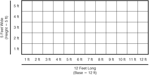
FIGURE 1-7 • Shape of a Bathroom

In order to find the appropriate amount of flooring to buy, we need to know the area of the bathroom. To find the area of a rectangle, we simply calculate the following:

For our bathroom, the length is 12 feet and the width is 5 feet, so the area is . It would take 60 square feet of flooring in order to cover this area. Suppose the local hardware store sold square tiles that were 1 foot on each side (or the area of each tile was ). It would therefore take 60 of these tiles to cover the floor.

Now let’s consider an example that uses a graph. Suppose Margaret is selling pies for $6 each, so every time she sells a pie, she gets another $6. If she sells 5 pies, she makes a total of $30 (from ). We could create a graph that shows how much money she earns (also called revenue). Figure 1-8 shows Margaret’s earnings. Point A represents the quantity that Margaret sells (5) and the price that Margaret gets ($6), and point A also defines a rectangle with a base of 5 and a height of $6. When we find the area of that rectangle, we are finding the revenue that Margaret earns. Areas of rectangles can illustrate economic variables such as total earnings (or conversely, the total amount of spending), and also profit.

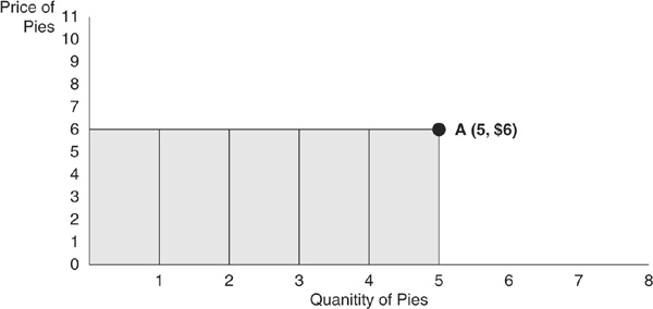
FIGURE 1-8 • Margaret’s Revenue from Pies

The other common area you will need to calculate is the area of a triangle. Economists often use triangles to describe consumer and producer surplus. Suppose there is another room in your house that is 8 feet long and 15 feet wide, but you want to divide the room in half so that there are two triangles of different-colored flooring. Figure 1-9 shows just such a room.

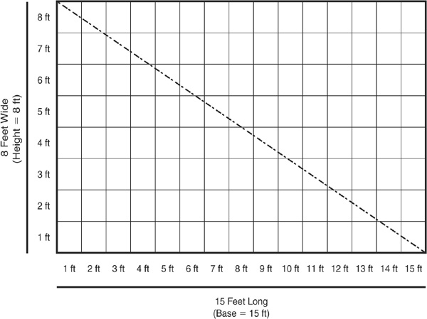
FIGURE 1-9 • Room with Two Flooring Colors

Note that if we were going to just tile the entire room the same color, we would need to find out the area of this rectangular room. Intuitively, if we want to tile only half of the room a particular color, we will need to calculate the area of half of the room. If you notice, every rectangle (or square) can be broken down into two triangles. It makes sense, then, that to find the area of a triangle, we find the area of the entire rectangle and divide by 2:

In our example, then, to tile half the room, we would need of tile.

Occasionally, you will see more complicated shapes, such as the shaded trapezoid that appears in Figure 1-10. The good news is even complicated shapes such as this can be broken down into triangles and rectangles, and the area can easily be calculated. Try to figure out the area of the shaded trapezoid in Figure 1-10 (we’ll give you the solution at the end of the appendix).

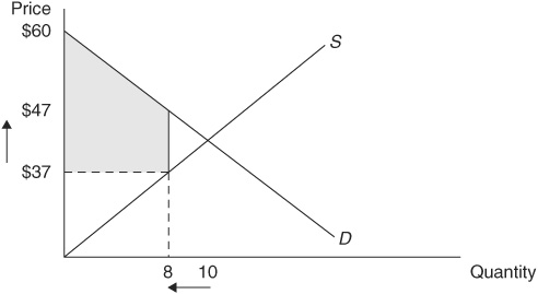
FIGURE 1-10 • A Market with a Price Floor

Solving Equations

Traditionally, a line represented on a graph is given as , where either y is known and you solve for x, or x is known and you solve for y. For instance, you could have the function:

If we are given that , we can solve this by substituting 5 for the x:

Conversely, if we are told that , we can solve to find the value of x that corresponds to :

First, isolate the term with x in it so that it is by itself on one side of the equation by subtracting 2 from each side:

Second, isolate x itself by dividing both sides by 3:

When you have a single equation with a single unknown, this is a fairly straightforward process. Note that this can be done no matter what way you express an equation. For instance, instead of , you could say that the quantity of a good that someone is willing to buy is a function of its price, , or that the cost of producing a good is a function of the quantity produced, Cost = f(q), and so on.

Also, we can solve such an equation only if we are given one of the unknown values. A function such as has two unknowns, x and y. In fact, we can generalize this rule to describe what we need to do in order to solve any system of equations (that is, a set of one or more equations) to find the unknown values. The equation would be a system of one equation with one unknown value (x), so we can solve this system quickly. However, if we were given only , we could not solve this because it is a system of one equation with two unknown values. In general, in order to be able to solve for all of the unknown values in a system of equations, there must be at least as many equations as there are unknowns.

For example, suppose we are given the following system of equations:

Here we have a system of two equations with two unknowns (x and y), so we can solve for both of the unknowns. To do so is fairly straightforward. First, we know that , so we can set these two equations equal:

Second, we want all of the x terms on one side of the equation, so we subtract 2x from each side:

Next, we want to isolate the x terms, so we subtract 2 from each side:

Finally, we solve for x by dividing both sides of the equation by 8:

To find the remaining unknown, we simply plug into either of the original equations. It doesn’t matter which one; we will get the same result:

Solving a system of two equations is particularly useful when we are talking about market equilibrium. Supply and demand are both equations in which the price and quantity are unknown values. In a market, we could express supply and demand as a system of two equations. For instance, suppose we knew that the market for a good was described by the following supply and demand functions:

At first this seems unsolvable: we have two equations (supply and demand), but four unknowns (P_s, P_d, Q_s, and Q_d). All is not lost, however. When we try to find equilibrium in a market, what we are really trying to do is to find a single price (that buyers will pay and sellers will get) that will make the quantity supplied and the quantity demanded the same. Translating that statement into an equation, we are assuming that:

There exists some P where
There exists some Q where

We can then substitute P and Q into the system of equations:

Now we have a solvable system! Go ahead and try to find the equilibrium price and quantity in this market (we will give you the answers at the end of the appendix).

Still Struggling

Math is like a language; the more you practice it, the better you get. If you are struggling with math, take your time, do extra practice, and know that you are not alone.

Answers and Explanations for Practice Problems

The first bit of practice we asked you to try was to find the equation of the line, in the form , in Figure 1-1b. This is a line that passes through two points: (0, 4) and (4, 0). We can do this a few different ways.

The first method is to examine the graph, get the y intercept from the graph, and use the line to calculate the slope. To find the y intercept, a in the equation, we find the value where the line crosses the y axis. In Figure 1-1b, the line crosses the y axis at 4, so . You might have once learned that the slope of a line is “rise over run.” In other words, for every 1-unit change in the length of the curve, the slope tells us the change in the height of the curve. In this case, it is fairly simple: every time x decreases by 1 unit, y increases by 1 unit, so . This gives us the equation .

The other way to solve this is to recognize that the equation is an equation with four unknown values (a, b, x, and y). The points and each independently solve :

We can now solve this system of two equations in two unknowns (a and b). First, isolate a in one of the equations. This is easy in this case, since . Therefore, from the first point, . We can now plug this value of a into the second equation:

Next, we asked you to try to find the area of the trapezoid in Figure 1-10. If you draw a straight line across (as shown in Figure 1-11) from a price of $47, the shaded area is now made up of two shapes: a triangle with a height of and a base of 8 units, and a rectangle with a height of and a base of 8 units.

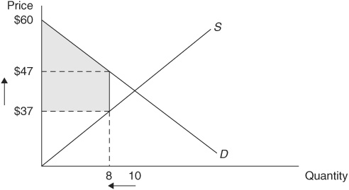
FIGURE 1-11 • A Market with a Price Floor

We now simply find the area of the triangle and the area of the rectangle and add these two areas together:

Finally, we asked you to solve for a market equilibrium with a supply curve of and a demand curve of . Start by noting that and setting the two equations equal to each other:

Next, isolate the Q terms on one side of the equation, so add Q to both sides of the equation:

Now isolate Q by subtracting 2 from each side:

Finally, solve for Q by dividing each side by 3:

To find the equilibrium price, simply plug into either the supply or the demand function:

Therefore, we find that the equilibrium in this market occurs when the price is $26, and at that price, 12 units will be sold.

QUIZ

Is each of the following statements true or false? Explain.

1. Money is an economic resource.

2. Even if the monetary price of a Ferb is $100, this may not reflect its true cost.

3. The producer of a good who is thinking rationally will focus on the average cost of producing a good.

4. Decision making by households is in the realm of microeconomics, while decision making by large firms is in the realm of macroeconomics.

5. The price of a purplett is $9, the additional benefit from purchasing another purplett is $10, and the average benefit from purchasing another purplett is only $8. Given this, a buyer should not buy another purplett.

For each of the following, choose the answer that best fits.

6. Ceteris paribus means:

A. Nothing changes.

B. All else equal.

C. Rational thinking.

D. Opportunity cost.

7. Scharf sells T-shirts. When she sells 35 T-shirts, it costs her a total of $40, and when she sells 36 T-shirts, it costs her a total of $45. Based on this information, which of the following is definitely true?

A. It would be irrational for Scharf to sell any T-shirts for less than $40.

B. It would be irrational for Scharf to sell the thirty-sixth T-shirt unless she received at least $45 for it.

C. Scharf shouldn’t sell T-shirts, as it will never be possible for her to make a profit.

D. It would be irrational for Scharf to sell the thirty-sixth T-shirt unless she received at least $5 for it.

8. Which of the following would be considered capital?

A. The money raised to start a business.

B. A factory.

C. A worker.

D. Electricity.

9. Ruby, as a rational consumer, does not:

A. Intentionally make herself worse off.

B. Try to maximize her net benefit from consuming goods and services.

C. Ever consume the wrong amount.

D. Think marginally.

10. Scarcity is defined as:

A. The sum total of all economic resources.

B. The difference between the marginal costs and marginal benefits of an action.

C. The difference between unlimited wants and limited resources.

D. The difference between the price of a product and the cost of producing it.