THE SAYING “MEN PLAN AND GOD LAUGHS” COMES FROM the Ashkenazim. At the most elementary level we all know this is true. Some may believe God is just fickle and cruel. I don’t, but given the structure of the universe and the sordid history of our species, I understand how some arrive at that conclusion. Even if it were true, we would be no nearer to understanding why contingency has played such an important role in the history of life on this planet and the history of social events within one of its species, Homo sapiens.

Contingency played a role in bringing me to Ann Arbor in the fall of 1979. I was familiar with the University of Michigan from my visits to the campus when I was playing on Oberlin’s volleyball team. I was impressed, and as I mentioned in Chapter 2, I enjoyed the feel of Michigan more than that of Harvard Yard. I will always remember the moment the plane touched down at Detroit Metropolitan Airport in the summer of 1979. John “Jack” B. Burch of the Mollusk Division in the Department of Ecology and Evolutionary Biology (DEEB) picked me up and drove me to Ann Arbor.¹ Everything I owned was packed in a large black trunk and one suitcase (including my portable black-and-white TV and the pliers I used to turn its knob). Jack let me stay in his house until I got my first paycheck and could find an apartment.

Michigan’s department was divided between those in ecology, most of whom resided in the Natural Science Building across from the Bell Tower, and those in evolutionary biology and classical zoology, who were housed in the Museum of Zoology down the street. The department included some giants in the field of evolutionary biology, including Peter and Rosemary Grant (The Beak of the Finch), William D. Hamilton (declining force of natural selection, kin selection), Richard Alexander (sociobiology), and Arnold Kluge (cladistics).² I started my research with Jack Burch at the museum. However, I was most attracted to the thinking of the ecologists, particularly Beverly Rathcke (community ecology) and John Vandermeer (population ecology).

To say the least, I wasn’t in Kansas (Lowell) anymore. I was surrounded by some of the world’s most brilliant minds (much more than I had been at Oberlin). I was initially overcome by imposter syndrome of the racial variety. Many of the white students believed that the Black students were only there to meet affirmative action quotas, and some had no problem verbalizing that view. I almost believed it myself, until one of the faculty in the Mollusk Division informed me that of all the graduate students DEEB had admitted that year, I had scored highest on the GRE Analytical Reasoning section. I would later learn that some of my classmates suffered from imposter syndromes of other types (such as the gender kind). The graduate student pool in our department was ridiculously talented (even the students who never earned their PhDs). Nancy Moran, Trevor Price, Dolph Shluter, Tom Getty, Marlene Zuk, Peter Rosset, Cruz Phillips, Brian Schultz, and Mike Hanson were just a few of the brilliant students there at the time. My imposter syndrome was alleviated when I began to observe that some of the great minds were beginning to recognize the significance of my ideas. For example, before I arrived, Bill Hamilton had expressed no interest in the evolutionary impact of parasitism on host fitness. However, I floated (but never really pursued) this idea in a number of seminars during my first year at Michigan. Hamilton and his students would eventually go on to do groundbreaking work on this problem.³ It is entirely possible that he was already thinking about this problem before I arrived at Michigan, and my comments might have supplied the impetus to pursue the problem more seriously. Or investigating the impact of parasites on host fitness could have been Marlene Zuk’s idea. I had a number of conversations with her about a variety of things during those years. Somewhere I still have the purple pencil she gave me inscribed with the words “SMASH THE STATE.” I took those words to heart.

ORDER IS THE ENEMY OF CHAOS, BUT THE ENEMY OF ORDER IS ALSO THE ENEMY OF CHAOS.

—GREGOR MARKOWITZ, FROM NORMAN SPINRAD’S NOVEL AGENT OF CHAOS, 1988

Norman Spinrad’s Agent of Chaos is a science fiction novel that addresses the question of whether human social institutions can maintain themselves.⁴ The plot revolves around a totalitarian solar system government whose desire to create maximum stability ultimately gives rise to its destruction. In one of my favorite arcs in the Marvel Comic Universe, Dr. Strange battles the dreaded Dormammu, who is serving as the agent of Lord Chaos. Lord Chaos is engaged with Odin (Thor’s dad) in a universal chess game to determine the balance of order and chaos in the universe. What’s not to love about that plot? Finally, many people are familiar with the mathematical concept of chaos from Ian Malcolm (the fictional mathematician played by Jeff Goldblum in Jurassic Park). Similarly to Agent of Chaos, the movie ends with self-caused destruction: the demise of Jurassic Park results from the hubris of John Hammond and, especially, of InGen’s lead geneticist, Henry Wu. Throughout, Malcolm warns them that “nature always finds a way.”

To understand chaos (and why it’s so important), I need to take you through some basic mathematics. I know that for many readers, especially women and racially subordinated persons, the word “math” brings to mind the horrible experiences of their middle school and high school mathematics courses. The term for it is “math phobia,” and it results not from the fact that math is intrinsically difficult but from the often-inadequate pedagogy that has been deployed in teaching it. Fear not; I am going to describe how chaos works by first taking you back to some of the simplest math you ever learned. After that I will attempt to scaffold each step along my description in as nonthreatening a way as possible.

In middle school you learned about linear functions. In math a function is a relationship between a set of inputs and outputs. For linear functions, one input (call it x) gives you exactly one output (call it y). This means that the functions are also deterministic—simply put, one x gives you one y (Table 3.1). If you were to graph this function, it would result in a straight-line graph following the general equation y = mx + b (where m is the slope, or rise over run, and b is the point at which the function intercepts the Y-axis). The fact that such functions result in straight lines is why they are called linear. Linear functions also do not have variables with power exponents; another way of understanding it is that the exponent of linear equations is always 1 (so you could write the general equation as y = mx¹ + b). Finally, linear functions also follow two rules: (1) f(x + y) = f(x) + f(y); another way of saying this is that the function of two variables added together is equivalent to adding together the results of that function of each variable taken separately; and (2) f(ax) = a × f(x); another way of saying this is that the function of a constant number (here, called a) multiplied by a variable is the same as multiplying the constant times the function of the variable (Tables 3.2 and 3.3.). Linear functions have a variety of applications in science, describing a dizzying array of natural phenomena. For example, the relationship between an adult individual’s height and weight is generally linear, and the relationship between a quantitative trait of offspring and the average of that trait between the biological parents is generally linear. In reality, linearity is nature well-behaved, but we all know that nature does not behave well very often.

Table 3.1 Simple deterministic linear function y = x + 5

x	y
0	5
1	6
2	7
3	8

Table 3.2 Associative rule of linear functions

x₁	x₂	f(x₁)	f(x₂)	f(x₁) + f(x₂)	f(x₁ + x₂)
0	5	0	10	10	2 × 5 = 10
1	6	2	12	14	2 × 7 = 14
2	7	4	14	18	2 × 9 = 18
3	8	6	16	22	2 × 11 = 22

The results of the function y = mx + b are shown, calculated by f(x₁ + x₂) and by f(x₁) + f(x₂), where m = 2 and b = 0.

Table 3.3 Commutative rule of linear functions

x	a	ax	y = f(ax)	a × f(x)
0	2	0	0	2 × 0 = 0
1	2	2	4	2 × 2 = 4
2	2	4	8	2 × 4 = 8
3	2	6	12	2 × 6 = 12

The results of the function y = mx + b are shown, calculated by f(ax) and by a × f(x), where a = 2, m = 2, and b = 0.

Nonlinear functions do not obey these rules and have exponents. Some of the most significant and not well-behaved phenomena in nature are governed by nonlinear dynamics. The system in which chaos was first discovered was weather. In the early 1960s the meteorologist Edward Lorenz was using a computer to try to predict the weather. Lorenz’s idea was that weather could be predicted by measuring three essential variables in the atmosphere: temperature, pressure, and humidity. He constructed a simple mathematical model to predict the weather. However, he noticed that as his computer began to calculate, small variations in its predictions began to appear between models. The variations were seemingly unexplainable by his deterministic models. After all, one x was supposed to produce one y. The variations appeared because the machine was computing answers to more decimal places than appeared on his readout; for example, the readout might show 0.321, but the answer was actually 0.321546. It turned out that the small difference between 0.321000 and 0.321546 mattered.⁵ The functions were still deterministic, but they were producing a complex outcome that Lorenz had not anticipated.

I first encountered this problem in population dynamics. Ecologists had long known that the populations of small organisms such as insects, snails, and crustaceans varied from year to year. The prevailing explanation for this was that factors of the physical environment randomly varied from year to year. These variations in turn would affect the survival and reproduction of the organisms in question. It turned out the explanation wasn’t quite that simple. I was first introduced to this question by a lecture given in our department by Princeton mathematician and ecologist Robert May. May was a physicist by training, but he became interested in problems in population biology. Specifically, he had begun working with a simple equation that modeled density-dependent population growth. Density dependence means that a population’s rate of growth is influenced by its own numbers. As the population numbers per area or volume increase (increasing density), either resources are exhausted, individuals produce toxins, or some other mechanism feeds back on members of the population and reduces their rate of increase. A simple example of this is what we observe when bacteria are growing in a vial with limited food. They divide by binary fission (splitting in two), and in theory this should lead to exponential growth. If even one bacterium grew in this way, then the earth would eventually be covered by that one bacterial species. However, this doesn’t happen; rather, bacterial growth in culture shows a lag phase, followed by exponential growth, followed by a stationary phase. (Panel A of Figure 3.1 shows a calculation of the discrete logistic equation May proposed for modeling population growth.) In these simple systems, bacteria go into a stationary phase (and will eventually die) because of resource exhaustion.

Density-dependent population growth is seen in virtually all real-world organisms (including humans, but that’s a more complicated kettle of worms to get into). May’s discrete logistic equation for modeling population growth has some surprising features. It is an example of an equation whose equilibrium outcome is determined by the initial variables (parameters) used. In population growth models, the term “equilibrium” refers to the point at which the rate of change is zero (or population size does not change anymore). The panels in Figure 3.1 show what happens to this simple equation when the value of its r parameter is increased; r is the intrinsic rate of growth that is determined by the instantaneous birth (b) and death (d) rates such that r = b − d. The figure illustrates that a population whose birth rate is greater than its death rate will grow, and the opposite situation will cause the population to decline. Zero population growth would occur in the case of b = d. (All this assumes that migration rates are balanced—the number entering is the same as the number leaving.) In Figure 3.1, panel A (r = 1.0), the population grows to its carrying capacity (the number of individuals the environment’s resources can support). In Figure 3.1, panel B (r = 1.9), the population overshoots its capacity, but oscillates back to the level predicted by its carrying capacity. However, in Figure 3.1, panel C (r = 2.1), we see a new behavior, with a two-point cycle appearing. The population exceeds its capacity, then drops below it, and then exceeds it, ad infinitum. Finally, in Figure 3.1, panel D (r = 2.6), the population exhibits a four-point cycle. Furthermore, as one increases the value of r beyond 2.6, a series of cycles of value 2ⁿ power (4, 8, 16…) can be generated in rapid succession. However, May showed that the discrete logistic took on an even more complex behavior at the value r = 2.693. At this value, you could theoretically find any integer-value cycle (e.g., 3) or an infinite series displaying no cycles. This behavior was entitled “chaos” after an early paper published by two mathematicians, Tien-Yien Li and James Yorke in 1975.⁶

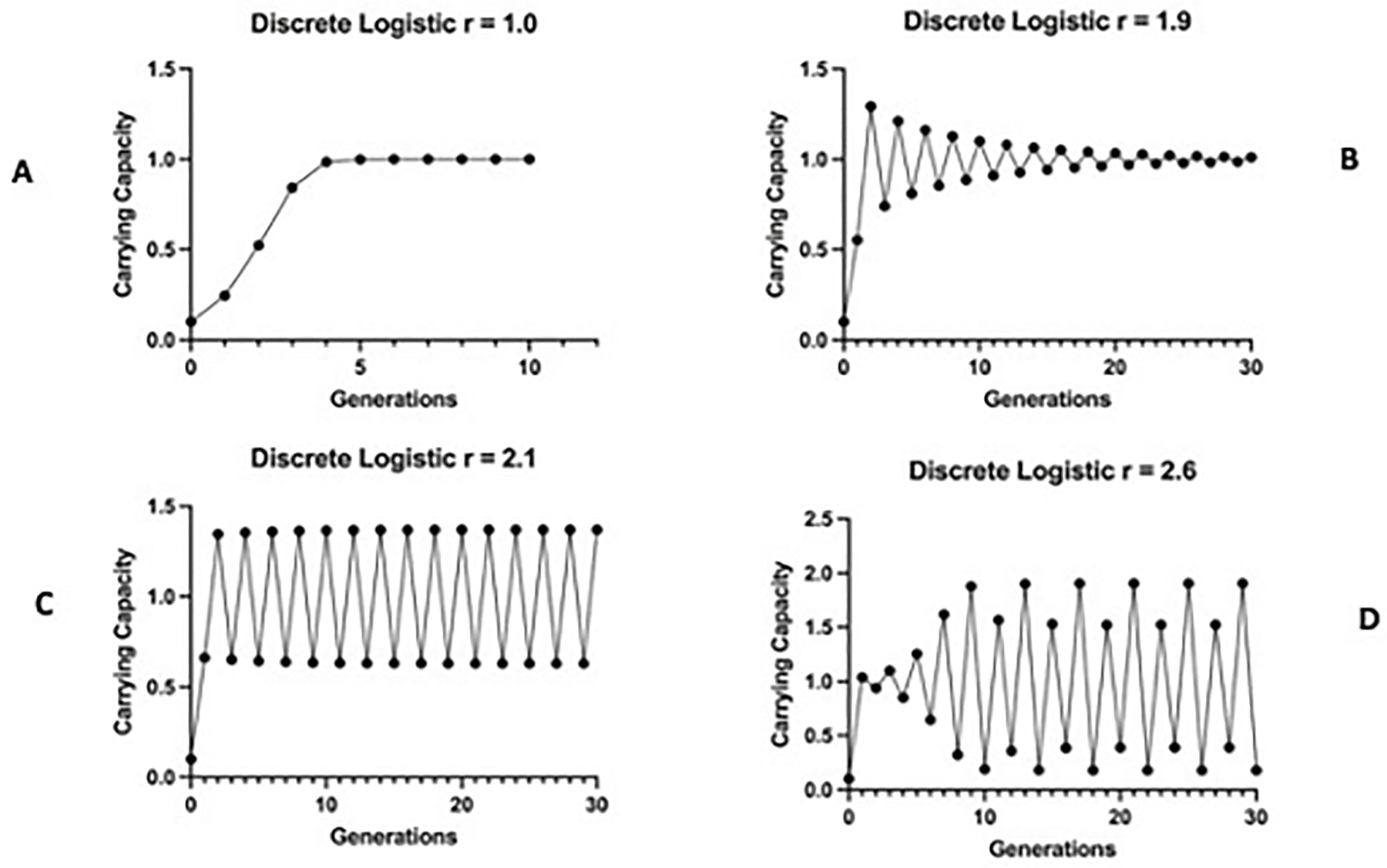
Figure 3.1. The discrete logistic equation calculated with different values of intrinsic rate of increase (r). The equation’s equilibrium outcome is determined by the value of r. In panel A, r = 1.0: the population settles on its carry capacity (K = 1.0, for all discrete logistic models). In panel B, r = 1.9: the population displays a damped equilibrium, oscillating above and below the K value and eventually settling on it. In panel C, r = 2.1: the population shows an expanding oscillation eventually settling on a two-point cycle. In panel D, r = 2.6: a four-point cycle is shown.

Furthermore, as Lorenz found with his weather equations, changing the initial value of the discrete logistic also changes the pattern of its outcome (Figure 3.2). The primary revelation of chaos theory was that the complexity observed in many systems could easily result from the interaction of very simple nonlinear functions. Lorenz had already shown that this was true for weather, with the underlying force being the phenomenon of turbulence, a chaotic fluid dynamic. May demonstrated the significance of chaos for biological populations. There seemed to be no end to the applications of this idea: the earth’s magnetic field, economic cycles, galactic orbits, financing of governments, neural control of the human heart, and the periodicity of ice ages.⁷ One in particular impressed me: Alvin Saperstein’s arguments that arms races were inherently chaotic and would necessarily drag nations into war.⁸

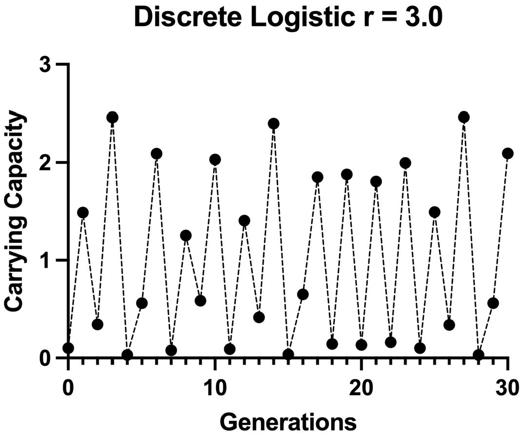
Figure 3.2. The discrete logistic equation (in chaotic regime). The equation is calculated with the intrinsic rate of increase r = 3.0. At r > 2.693, any period cycle (or no cycle) can occur. This population dynamic is labeled “chaos.”

DURING MY UNDERGRADUATE AND MASTER’S WORK I HAD ALREADY recognized the overarching significance of mathematical thinking in biology. So it was no surprise that I was attracted to Robert May’s ideas.⁹ I attended May’s lecture at the same time I was enrolled in John Vandermeer’s mathematical ecology class. John was an intellectual descendant of the founders of modern ecology. He wrote one of the first doctoral theses to utilize an analysis of variance in an ecological study. Prior to his generation, ecology was more descriptive than quantitative. We were the first class to use his text in mathematical ecology; we proofread it for errors before its first publication.¹⁰

The preliminary exam for the progression to PhD candidacy at Michigan was organized around a review paper. It was expected that the review would be suitable for publication in a major professional journal. I had already been working on some population experiments with Biomphalaria glabrata (snails) at the museum to see if I could generate chaotic population behavior. I grew the snails at a series of densities and collected their progeny in a narrow window to simulate discrete generations (as required by the discrete logistic equation). The density levels were plotted on the X-axis as n_t and their offspring numbers on the Y-axis as n_{t + 1}. The angle at which the resulting plot crossed the identity line (n_t = n_{t + 1}) provided a prediction of whether the system would display a stable point, damped equilibrium, cycles, or chaos (Figure 3.3). The data I collected did not support the idea that this species, under the conditions I was growing it, would show any sort of population oscillation.

Figure 3.3. Model of competition between two species with the discrete logistic equation. The outcome of the species’ dynamics is determined by the interaction between the values of intrinsic rate of increase (r₁, r₂) and the competition coefficients (a₁₂, b₂₁). In panel A, r values for both species are less than 1.0, with mild competition, resulting in a damped oscillation and persistence of both species. In panel B, r values are greater than 1.0, with mild competition, generating a two-point cycle. Both species persist, but the oscillations are such that in a real-world scenario both would be likely to go extinct as a result of their interaction. Thus, the discrete logistic competition model shifts the origin of complex behavior to much lower values of r compared to the one-species model.

The results of this experiment indicated that a very prolifically reproducing species grown in conditions of high nutrition and in the absence of parasites and predators did not show chaotic dynamics. However, this situation got me to think more deeply about the way species actually live in nature. Obviously, species do not exist in nature alone. For example, the snail B. glabrata lived in communities with other snails of the same family (Planorbidae) that occupied similar ecological niches. Therefore, the topic of my review paper was to extend May’s single-species models to multiple-species interaction, specifically competition. Choosing this topic also meant breaking with Jack Burch as my primary adviser and switching to John Vandermeer. My interest in competition as a key force in natural communities was due to my interactions with Beverly Rathcke. To study this problem, I wrote the classical Lotka-Volterra (LV) competition equations in discrete form. John helped me study the behavior of these equations by writing a Fortran program that allowed me to alter the parameters of the competition equations, thus allowing me to predict which combinations of intrinsic rates of increase (r) and competition coefficients (a, b) resulted in reducing or expanding the realms of single equilibrium, stable cycles, and chaos. The algorithm John wrote for his program was a good start, but I spent a lot of time debugging that program. It turned out to have the same problem as Lorenz’s original calculations of weather. The algorithm was calculating answers out beyond ten decimal places. Thus, even if a cycle existed, it would take an inordinate amount of time for the system to recognize it. I decided to have the program round numbers to eight decimal places. With that modification, the program began to display the predicted behavior of the competition equations. This was time-consuming work, and as the date of my preliminary exam approached, I switched into MBL mode: I was sleeping only two to three hours a night, on a couch in John’s office. When I hadn’t returned home for two weeks, my roommates called the Ann Arbor police to inquire about filing a missing person report.

The study confirmed my general suspicion, that adding species interaction makes the landscape of population dynamics more complicated. In the LV competition model, there are two general possibilities: one species drives the other to extinction, or the two species coexist; which occurs depends upon the relationship of their initial comparative population sizes and their competition coefficients. The discrete logistic model by its formulation prevents formal extinction, although in practice species that take on very low fractions of their carrying capacity are likely to go extinct in the real world. The other major result my model showed was that the space in which stable equilibrium, 2ⁿ cycles, and chaos either expanded or contracted depended upon the relationship between the intrinsic rate of increase and the competition coefficients between the two species. For example, a species with a value of r that would predict chaotic dynamics in the single-species model could be pulled out of that regime by strong competition with a second species. Conversely, weak competition between competitors without sufficient r to bring them into chaos could also pull them into this regime. Furthermore, the more species that are placed in the model, the more unpredictable the results become.

My review paper was sufficient to pass my candidacy exam, but I never published the results of that work. Going into the exam I was pretty sure I was going to pass, as the committee was composed of Richard Alexander, Beverly Rathcke, and John Vandermeer. I didn’t know Alexander personally, but I was already at odds with the E. O. Wilson version of sociobiology.¹¹ Alexander also was an adherent of this theory. During the exam, he asked me to explain my paper in such a way that my mother might be able to understand it. I took offense to that, as I was absolutely sure he knew nothing about my background or my mother’s education. So I responded with something along the lines of “My mother holds a PhD in theoretical physics, so for her this work would be trivial. However, I can see that you don’t understand it, so I will happily break it down for you.” To Alexander’s credit and my great amazement, I passed the exam with a vote of 3–0.

MODELS ARE, AT THE END OF THE DAY, ONLY SIMULATIONS THAT represent possible reality. This is something Rathcke taught me. Models are mostly useful when they make predictions that can be tested by experiment. Furthermore, she taught me that we had to look very carefully at experiments to make sure their design would really test the predictions of the models that spawned them. Despite those caveats, I was so enamored with the mathematical elegance of chaos theory that I was ignoring the result of my own experiments. The snail experiment I ran did not produce data indicating that this species, growing under favorable laboratory conditions (adequate, high-quality food; controlled temperature; few parasites; fresh water), was showing an intrinsic rate of increase capable of generating chaotic dynamics. Nor did I know that at the same time I was running my experiment, my future colleague Larry Mueller was conducting a similar experiment using several strains of fruit fly (Drosophila).¹² His results also indicated that the vast majority of these strains were not generating intrinsic rates of increase that would support the claim that their population dynamics should be chaotic.

Of course, I rationalized my single-species results (as predicted by my multispecies model) by explaining that they were not necessarily indicative of what would happen in complex multispecies assemblies. In my review paper, I had considered how evolution and genetic variation might influence multispecies dynamics. My modeling also suggested that genetic changes in life history (a term I didn’t fully understand yet) would contribute to even more chaotic dynamics. At the end of the day, I had thoroughly convinced myself that the “new science” of chaos was at the root of all population interactions occurring in nature (as least in organisms with high intrinsic rates of increase). The rest of the department dubbed me “Dr. Chaos.” I remember that my insistence on the significance of chaotic population dynamics undergirding so much of nature really rubbed senior graduate student Tom Getty (now a professor and colleague at Michigan State University) the wrong way. To my great surprise, at my last seminar in the department everyone had in front of them a chocolate bar and a bottle of Coca-Cola (my lunch of choice in those days), and Beverly presented me with a customized red T-shirt with “Dr. Chaos” across the front.

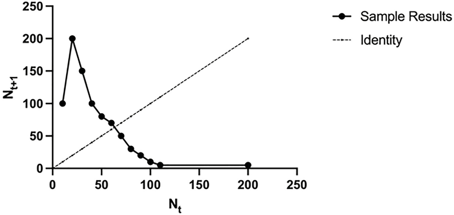
Figure 3.4. Sample data illustrating how one can estimate whether density-dependent growth would predict chaotic population dynamics. To predict the dynamics, begin at any point on the n_t axis, go up to the dotted curve (n_t+1), then over to the identity line. Repeat this process. If the path you trace settles on the point where the dotted curve crosses the identity line, then this curve predicts one stable equilibrium point. Alternatively, you could end up tracing a 2, 4, 8 (2ⁿ) cycle. And if you continue tracing with no cycle, the curve predicts chaotic dynamics. This example predicts chaos.

The levity I projected around my ideas was actually masking a much deeper disappointment with the field and, even more, with my capacity to solve real scientific problems. I was being drawn deeper and deeper into self-doubt. To the world around me I displayed a demonic genius, like a Richard Wright of population biology. Wright was a brilliant African American author whose psychological problems prevented him from achieving even greater accomplishments. Beneath it all was my growing alienation from the scientific community and disappointment in society. My life had become as chaotic as the dynamics of nature I believed in.

A REVIEW OF THE DIGITAL ARCHIVES OF THE MICHIGAN DAILY (the University of Michigan’s student newspaper) shows that I had begun to be a social activist almost as soon as I reached the Ann Arbor campus.¹³ Practical activism is pointless and futile unless it is directed by a theory of social change. It was in Ann Arbor that I first came into contact with the ideas of the group Science for the People, which began in 1969 as a radical group of scientists who came together to protest the Vietnam War. Its core premise was that science was not neutral but, rather, inherently political. Specifically, the scientific enterprise (as opposed to its core methods) always reflects the social interests of those engaged in its practice. This realization was the most important epiphany of my life. It explained all the frustrations I had experienced so far in my career. I now had a perspective to help me understand the alienation I was feeling from the academy and its mission. I had decided to pursue a scientific career to help people in need, not to prop up the systems of injustice in society. Most of the students I was in contact with couldn’t have cared less about social justice. The reason for their lack of attention to this cause was now obvious to me. For most of the white males I knew, this was clearly their society; why should they be concerned about its inequities? The white females I knew suffered from patriarchy, but for most of them their racial and class identity was too important to risk by challenging sexism. Or they thought they could challenge sexism without taking on issues of race and class.

I picked up a copy of Biology as a Social Weapon in Vandermeer’s office.¹⁴ You couldn’t miss this book’s maize-and-blue cover. Harvard geneticist Richard Lewontin wrote the introduction, “Biological Determinism as a Social Weapon.” When Lewontin died in 2021, Science for the People asked me to write the piece concerning the significance of his early studies on human genetic variation.¹⁵ The chapters in Biology as a Social Weapon dealt with topics such as IQ and scientific racism, biological determinism and sexism, and sociobiology as the new biological determinism. All at once I recognized the failures of my previous education. As Denzel Washington’s paraphrased speech in the movie Malcolm X put it, I felt I had been “hoodwinked and bamboozled” by the paradigm of an apolitical academic science. Soon after reading Biology as a Social Weapon I read Allan Chase’s The Legacy of Malthus: The Social Costs of the New Scientific Racism.¹⁶ This book detailed the long history of biological deterministic racism in the United States. It gave example after example of the way racist lies dressed up as objective science had contributed to the ongoing suppression and death of racialized people in the United States.

These works caused me to ask serious questions about what my career and life were going to be about. Since the moment I graduated from college, I had been struggling with my mirror. Every morning I would get up and prepare for my day. But I avoided looking into my eyes for any extended period of time, because I wasn’t proud of who I was. The image of my mother stooping over to drag heavy boxes in the plastics factory haunted me. The daily insults I watched my father endure to keep food on our table echoed through my mind. I was at war with my better angel. I don’t remember the exact day, but I do know that one day I finally looked at myself in the mirror and confronted myself. On that day I made the decision to devote myself to the pursuit of justice. I began to read voraciously about people whose ideas had been denied to me in my previous education: Karl Marx, Lenin, Leon Trotsky, Rosa Luxemburg, Angela Davis, Malcolm X, Frantz Fanon, Sojourner Truth, and a host of others. By the time I was done, I had a very good idea of what was wrong with society, even if not so perfect an idea of how to fix it.

The day with the mirror significantly changed the trajectory of my career. The combination of being part of Vandermeer’s research group and ongoing campus struggles changed the focus of my interests. Two of these campus struggles were particularly important in determining the person I was becoming: the second Black Action Movement (BAM) protest and the Graduate Employees Organization (GEO) struggles.

African American students organized the first BAM protest in 1970. Their goal was to better their situation at the University of Michigan. They called for the administration to commit to increasing the representation of African Americans on campus to at least 10 percent of the student body by 1973–1974. They also asked for recruiters and for tutoring and counseling for these students. Finally, they asked for increased funding to support the Center for African American Studies (CAAS). The administration’s failure to act on these demands led to the first BAM strike, which began on March 19, 1970. BAM called for students to boycott classes. By the twenty-seventh, class attendance in the College of Literature, Science, and Arts (LSA) was down to 25 percent. Individuals had taken to acts of disruption, such as randomly reshelving fifteen thousand to twenty thousand books in the wrong sections of the Undergraduate Library (UGLI).¹⁷ The struggle escalated, and BAM participants were accused of doing serious damage to university buildings. The university eventually agreed (in principle, but not in action) to the BAM demands.

The GEO struggle began in earnest in 1973.¹⁸ The university had imposed a 24 percent tuition hike, resulting in a $3 million surplus, little of which went to supporting graduate education. The graduate students taught as many students as the faculty, but at one-fifth the cost. The movement for a graduate student union was based on this disparity; the university argued (as most still do) that teaching is part of graduate students’ training. By 1975 union fever was at a boil. In February of that year, GEO demanded the expansion of affirmative action at Michigan but received no response from the administration. On the tenth, GEO membership voted to strike (689–193). The next day they were picketing twenty-five to thirty buildings, class attendance was down 50 percent, and the union had support from African American student and staff groups, who had their own grievances against the university. As the strike intensified, property damage began to occur, such as tires being slashed on university vehicles and locks being sabotaged in university buildings. The fourteenth saw a mass rally with more than 2,500 protestors and a march on the president’s house. On the eighteenth 250 underrepresented minority students of the Third World Coalition occupied the second floor of the administration building (with GEO in support). The arrests of GEO picketers began near the end of the month. In early March representatives of GEO and the university met with a state-appointed arbitrator.¹⁹

When I arrived on campus in the fall of 1979, the BAM and GEO issues were unresolved. One only had to look around to see how few Black faces there were on campus, particularly in the LSA graduate program. There were probably only about five of us in STEM fields (that’s people, not percent). In this atmosphere it didn’t take much to get me involved in left-wing student activism, especially in light of all the fresh scars I bore from my time in Massachusetts. In a recent search of the digital archives of the Michigan Daily, I found my name mentioned in many articles associated with participation in (1979–1980) and then leadership of (1981–1983) Black Student Union– and GEO-related issues. The letter in Figure 3.5 was authored by me, and it was directed toward the disparate coverage that the Michigan Daily provided to white and Black issues on campus. I began in GEO as a shop steward for my department but was eventually elected to its steering committee. The university had negotiated a contract with GEO in 1976 but used a variety of sophistical tricks to avoid signing it. I was part of the GEO steering committee that eventually got the university to sign the contract on November 23, 1981. This was the first contract of its kind (i.e., between a university and its graduate student employees).

The second BAM protest was more of a demonstration than a movement, in the way that the first had been.²⁰ A search of the digital archives of the Michigan Daily for 1979–1983 did not find it mentioned specifically, although Melba Boyd did discuss it in her article “A Horse of a Different Color.”²¹ Rather, there are stories in the Daily about a series of related causes and incidents that I was involved in, including the Leo Kelly Defense Committee, Minority Fightback, and Black Student Union. It is also hard to assess the impact of the second BAM, but within a year of my leaving the university, it hired an unprecedented number of African American faculty. This was one of the demands that the second BAM forwarded to the administration.

Figure 3.5. “Daily insensitive to minority issues”

THE UNIVERSITY OF MICHIGAN DID NOT KILL ME, BUT MY POLITICAL activity came at a cost. I was growing more and more cynical about the prospect that the United States (or world) would achieve a just society. My disillusionment with society fed back onto a disillusionment with myself, specifically my ability to perform in my major. This, in conjunction with the massive amount of time I was spending on political causes, meant that I was rarely attending class. My bitterness came through not only against my opponents but also with my friends. A simple read of Daily articles concerning GEO and its negotiations with the university showed the growing animosity between me and the moderates in the union leadership.²² At some point, as I recall, someone described me as “a self-styled Marxist-Leninist” who was “the most dangerous man on campus.” Certainly by 1983 I had taken up some of the most controversial positions and causes on campus, including being part of the Leo Kelly Defense Committee.²³ Kelly (a Black student) was charged in the shooting of two white students. His defense attorney claimed he had been loaded up on pills at the time of the shooting. Our committee never claimed that Kelly had not committed the crime; rather, we argued that the crime had occurred in the context of the racially hostile climate of the University of Michigan. We also pointed to the racist treatment he was receiving at the hands of the courts, including being put on trial before an all-white jury (the only jury one was likely to have in Washtenaw County). In my statement to the Daily I said, “The real person who pulled the trigger is institutional racism at the University of Michigan.”²⁴

At this point, my personal state was rapidly unraveling, in much the same way the universe was supposed to behave in Spinrad’s Agent of Chaos: “It is simplistic to equate chaos with what is vaguely called the Natural State. Chaos underlies the increasing entropy of the raw universe, to be sure, but it also fills every interstice in that most defiant of anti-entropic constructs—Ordered human society.”²⁵ It soon became clear that the combination of my disappointment with the state of ecological science research, the widespread resistance on campus to my role as a political activist, and growing distance from my friends and colleagues meant that there was no way forward for me at Michigan. In the last year of my time there I was no longer talking to John Vandermeer. What I thought were principled differences between us were really just the result of my own growing alienation from everything and everyone around me. It would be years before we would speak again. Rathcke remained an advocate for me. Eventually, the letter I knew was coming arrived from the graduate school. As I had essentially stopped attending classes, my grade point average had fallen below the 3.0 required to remain in the program. The university made no attempt to place me on probation, nor did it offer a discussion with anyone in the graduate school about how I might stay in the university. The letter was clear: I was no longer a student at the University of Michigan.

It would be unfair to say that my time at Michigan did not play a crucial role in the scientist and person I eventually became. Ironically, despite being engaged in constant struggle with the institution while I was there, I have very fond memories of that time. My first two years there I played with Michigan’s MIVA club volleyball team. It was refreshing to be finally playing with a team that had the talent to make a run for the MIVA championship. In my first year with the team we made it to the MIVA championship semifinals. We lost to Notre Dame in a heartbreaker played on our home court.

I met many of my closest lifelong friends at Michigan. I saw Beverly Rathcke there shortly before she passed away in 2011. Brad Pollack (who participated in the Black Student Union [BSU]) passed away in 2009. He was an Oberlin grad and a scholar of the work of W. E. B. DuBois; he introduced me to the significance of DuBois’s work. Cruz Phillips (who still works helping organize farm workers), attorney Kai DeGraaf (whom I met through the Latin America Solidarity Committee), Leslie Adadow (who supported a variety of social causes), and Patrick Mason (BSU member and professor of economics at Florida State University) remain lifelong friends. Most important, at Michigan I met my wife, Sue.

CHAPTER THREE

Men Plan and God Laughs

Why Dynamical Complexity Is at the Heart of Some of Our Most “Stormy” Problems