CHAPTER THIRTEEN

Evolution in Silico

OPEN THE POD BAY DOORS, HAL.

I AM SORRY, DAVE. I’M AFRAID I CAN’T DO THAT.

—ASTRONAUT DAVE BOWMAN AND HAL 9000, 2001: A SPACE ODYSSEY, 1968

THE SUFFICIENT DEFINITION OF LIFE INCLUDES THAT IT IS ORGANIZED, has a metabolism and a genetic code, and is self-replicating. On our planet, living things are carbon based. Living things also have hydrogen, nitrogen, oxygen, sulfur, and phosphorous as their main constituents. Trace elements include a number of metals, such as iron, magnesium, calcium, sodium, and manganese. Carbon’s capacity to give rise to the structure of living things results from its capacity to polymerize (form long chains). These long chains fall into four important categories: nucleic acids (information storing, enzymatic), proteins (structural, enzymatic, in rare cases information storing), carbohydrates (structural, energy containing), and lipids (structural, energy containing).

In my teaching I liked to challenge my students to think about how life might evolve on another planet. Part of this results from my longtime fascination with science fiction. You already know about my love for Star Trek. Years later I learned that the voice of the artificial intelligence on the USS Enterprise (NCC-1701) was that of actress Majel Barrett (who also played nurse Christine Chapel). The first science fiction novel I remember reading was Arthur C. Clarke’s Childhood’s End.¹ Clarke’s novel revolves around the end of the human species as it is subsumed into an ancient superintelligence. In the book, we never find out how the superintelligence evolved. However, what I know about evolution suggests that carbon-based life is not the only possibility. So a question I routinely put to my students is this: What about silicon-based life?

Silicon sits below carbon on the periodic table of the elements. It also is capable of forming four chemical bonds. Silicon makes up about 27.7 percent of the earth’s crust. Compare that to carbon, which only makes up about 0.025 percent of the earth’s crust and 0.041 percent of the earth’s atmosphere in CO₂ (at present). So why didn’t silicon-based life-forms evolve on this planet? The answer is simply that it doesn’t form polymers. It is a semiconducting metalloid and is generally highly unreactive (meaning it probably wouldn’t be able to produce a silicon-based metabolism, either). Semiconductors are materials that have an electrical conductivity between that of an insulator (e.g., rubber) and that of the metals. A metalloid is also, as it sounds, a material that has properties in between those of metals and nonmetals. So while silicon could never have been the element that would form the basis of living things on this planet, its semiconductor characteristics make it an excellent element to use in building computer chips. Such chips have made it much easier to compute the results of complex mathematical operations.

WHEN I BEGAN MY SCIENCE EDUCATION, WE USED SLIDE RULES to calculate the results of sophisticated mathematical operations. There is some debate about when the device was invented, but it was invented at least by sometime in the early seventeenth century, for Isaac Newton used a slide rule to make many of his calculations.² I started to learn how to write computer programs in BASIC when I was in high school. Computers at that time (and even when I was in college during the mid-1970s) were large machines that required major amounts of space and energy and many technicians to support them.³ The movement down from these computers to the personal computer began in 1969. Ted Hoff at Intel designed a general-purpose chip set: a read-only memory to permanently store data and applications (ROM, called 4001 chip); a random-access memory to hold data (RAM, 4002 chip); a chip to handle input and output (4003 chip); and the central-processing unit (CPU, chip 4004). The idea took off, and soon amateur computer hobbyists were building microcomputers.⁴ After hobbyists, start-up firms soon picked up the idea; most went out of business, but a few survived (such as Apple). The success of the Apple computer motivated International Business Machines (IBM, or HAL, if you advance each letter by one) to design their own PC. They started on the design in 1980, and the IBM PC hit the market in August 1981.⁵ The first time I saw a PC was right around that time in the Museum of Natural History at Michigan in the office of a new faculty member.

I didn’t actually use a PC until I was working on my doctoral dissertation. During my master’s work at Lowell, I was still writing Fortran programs to run statistical analyses. I used Robert Sokal and James Rohlf’s Introduction to Biostatistics to generate my lines of code for any given test.⁶ The nice thing about that book was that it had boxes designed to carry you through the calculation of each part of the analysis. To get the program to run, I simply used those boxes to generate my Fortran statements. The code was typed on punch cards that you then walked over to the computer center. This was still how I was getting my computing done when I worked with John Vandermeer at Michigan. John noticed right away that I was better at writing computer code than most of the other incoming students. Truth be told, I don’t consider myself to have great coding skills; I often use brute force to do things that a better coder could do with far fewer lines. However, at the end of the day, it is still better to have brute force code that works than to have to calculate that stuff yourself! I still have the book I originally used to learn Fortran on the shelf in my office.⁷

The first PC I worked on was an IBM PC, and I had to learn disk operating system (DOS) commands; graphical user interfaces (GUIs) were not yet in widespread use. DOS commands, which had to be typed in on a keyboard, allowed one to do the basics, such as listing the files on the computer, copying files, and making directories to store files. Obviously one could do more with DOS, but for my work that was about all I managed to use. I wrote my doctoral dissertation in a word-processing program called Volkswriter.⁸ However, the real boon for getting my thesis completed was the program Grapher. Grapher allowed me to make graphs of my results in a fraction of the time it took to do them by hand. There were over twenty-five graphs in my dissertation, so this really helped reduce the amount of time I spent making figures. This software is still in use; I found a reference to it in a 2017 paper.⁹ Finally, spreadsheet applications became extremely useful, both in research and in teaching. I began using Lotus 1-2-3 software but later, like most people, I shifted to using Microsoft Excel.¹⁰ Spreadsheet applications are particularly useful for iterative (repetitive) calculations. I still use spreadsheets to help students learn how biological equations model phenomena in nature. This is a particularly useful approach for students who are computerphobic. For example, a simple tool for teaching students how natural selection acts on a deleterious recessive gene is shown in Table 13.1. Once again, this is a brute-force example of calculating the results of an equation. However, its heuristic value is that the student sees each calculation of the equation by parts. In addition, once the spreadsheet is saved, the student can return to it and change its parameter values or initial starting conditions to evaluate how it behaves (a ready-made parameter-study machine). The value of this approach has been recognized, as virtually any equation in ecology and evolution can be turned into a spreadsheet exercise.¹¹

Table 13.1. Selection against a deleterious recessive allele (by spreadsheet)

Gen.	s	q	p	q2	spq2	sq2	1 − sq2	Dq	q’	p’
0	0.900	0.990	0.01	0.980	0.009	0.882	0.118	0.075	0.915	0.085
1	0.900	0.915	0.085	0.838	0.064	0.754	0.246	0.260	0.656	0.344
2	0.900	0.656	0.344	0.430	0.133	0.387	0.613	0.217	0.438	0.562
3	0.900	0.438	0.562	0.192	0.097	0.173	0.827	0.117	0.321	0.679
4	0.900	0.321	0.679	0.103	0.063	0.093	0.907	0.069	0.252	0.748
5	0.900	0.252	0.748	0.063	0.043	0.057	0.943	0.045	0.206	0.792
6	0.900	0.206	0.792	0.043	0.030	0.038	0.962	0.032	0.175	0.825
7	0.900	0.175	0.825	0.031	0.023	0.027	0.973	0.023	0.151	0.849
8	0.900	0.151	0.849	0.023	0.018	0.021	0.979	0.018	0.134	0.866
9	0.900	0.134	0.866	0.018	0.014	0.016	0.984	0.011	0.119	0.881
10	0.900	0.119	0.881	0.014	0.011	0.013	0.987	0.009	0.108	0.892

Notes: Column 1 = Generations; this is filled by hand. Column 2 = s (a constant); initial value is entered by hand and then filled down. Column 3 = q; initial value is entered by hand, value in row 3 of the spreadsheet is assigned by column 10. Column 4, cell formula = 1.000 − C2. Column 5, cell formula = C2 × C2. Column 6, cell formula = B2 × D2 × E2. Column 7, cell formula = B2 × E2. Column 8, cell formula = 1.000 − G2. Column 9, cell formula = F2 / H2. Column 10, cell formula = C2 − I2. Column 11, cell formula = 1.000 − J2. Now the trick to make this an iterative spreadsheet is to make the cell formula for the C3 cell = J2. Then you fill down all remaining cells in the second row to the third row. Then fill down all rows from the third row to complete the entire spreadsheet.

This table shows the results of a spreadsheet written to iterate the calculation of allele frequency utilizing the equation for natural selection against a recessive allele: Dq = (spq²) / (1 − sq²). An example of this equation working in nature is the famous industrial melanism example (an increase in the number of dark-colored moths in response to pollution) of Bernard Kettlewell’s moths.

THE SECOND PAPER I CONTRIBUTED TO IN MY CAREER, PUBLISHED in 1988, attempted to localize the genes accounting for differences in life span in Drosophila melanogaster. Leo Luckinbill devised a series of crosses using the techniques of classical genetics to create a series of progeny lines containing different sets of chromosomes from the long- and short-lived stocks in his laboratory.¹² Drosophila have only three chromosomes, so the combinations of chromosomes would start with populations that had all their chromosomes from the long-lived stock (LLL) followed by combinations of two long and one short (SLL, LSL, LLS), and so on. Since we had already shown that life span was a genetically determined trait and that it was a quantitative trait, theory suggested that flies with the LLL genotype would live longer than flies of the two long and one short (SLL, LSL, LLS), two short and one long (SSL, SLS, and LSS), or three short (SSS) genotypes. The study generally confirmed this result (Figure 13.1). It also showed that chromosome 3 had the largest effect on increasing longevity and that this increase was enhanced by an epistatic effect of genes on chromosome 1. However, at this time, these crude estimates were the best we could do.

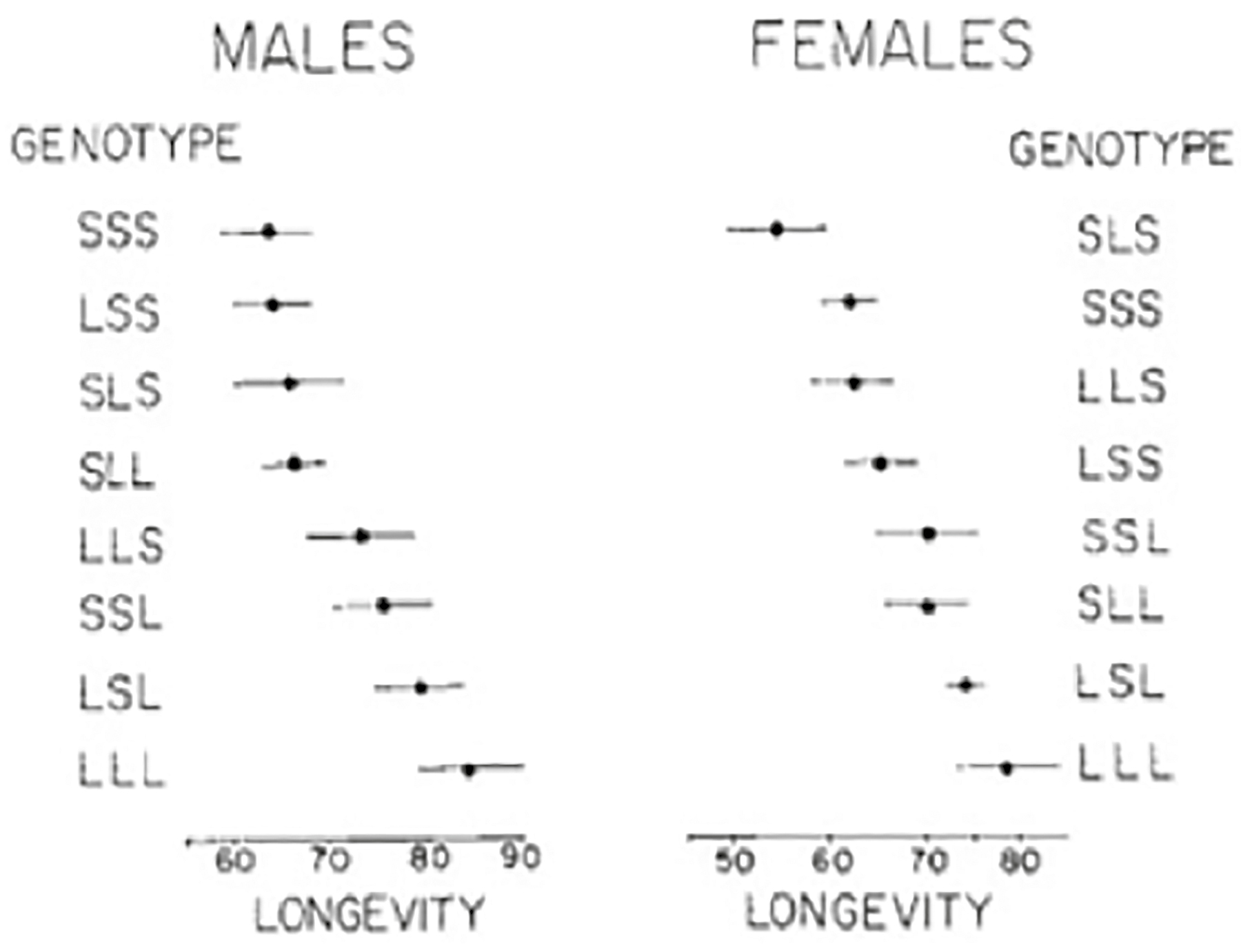
Figure 13.1. Mean and standard errors of life span for males and females (living alone) with different combinations of long- and short-lived chromosomes.
Source: Luckinbill LS et al., Localizing the genes that defer senescence in Drosophila melanogaster, Heredity 60 (1988): 367–374.

Five years later, Michael Rose’s group utilized the technique of two-dimensional electrophoresis to evaluate proteins that might be contributing to longer life span (postponed aging). This study was able to resolve 321 proteins that seemed to be differentially expressed in the short-lived (B) and long-lived (O) populations.¹³ Each one of these proteins was the product of a different gene, suggesting that at least 321 genes were playing a role in differentiating life span in Drosophila under selection for postponed senescence.

I describe these studies only to give the reader a sense of what our tools were like less than forty years ago to examine the relationship between the genotype and complex phenotypes. The Luckinbill study simply examined phenotypes; the Rose study improved on the approach by adding protein electrophoresis (still a phenotype). Each used what was then a state-of-the-art approach, because at the time of these studies, DNA sequencing by the Sanger and Maxam-Gilbert methods was too costly and time consuming. However, eventually all biological research would benefit from the spin-off technologies resulting from the desire to sequence the human genome. In 2004 the National Human Genome Research Institute (NHGRI) initiated a funding program whose goal was to reduce the cost of sequencing a human genome to $1,000 dollars in ten years.¹⁴ The technological advances in DNA sequencing are now recognized as next-generation sequencing (NGS). The methods utilize cell-free methods to prepare genomic libraries (or fragments of DNA) for sequencing, they utilize from thousands to many millions of sequencing reactions occurring in parallel, and sequencing output is detected without the use of electrophoresis. Thus, whole genomes can be sequenced at an amazing speed. For example, a few years back, my group, using a very underpowered NGS sequencing platform by today’s standards (the Illumina MiSeq), was still capable of sequencing the whole genomes of ten D. melanogaster populations in less than one week. We can generally do ten populations of the bacterium E. coli in about forty-eight hours. The drawback to NGS methods is that they produce short lengths of DNA to read, generally about 200–250 base pairs.¹⁵ You can watch the biochemistry of the Illumina sequencing by synthesis method on a YouTube video.¹⁶

By randomly cutting up pieces of DNA into small fragments, NGS methods generate a large amount of data to be analyzed. The first step is alignment. These algorithms utilize search tools to match the cut-up fragments with a reference genome. Initially, clever techniques had to be used to generate the reference genomes that we currently align to. However, with reference genomes, the process goes a lot faster. Once fragments are aligned, we can determine what is called depth of coverage, or how many times the fragments overlap the reference genome at a given point. The more fragments that map to a given place in the genome, the greater our confidence in determining that something does not match the reference at that point. For example, suppose that at a given position in the reference genome we are supposed to see an A (adenine), but instead, a given sequence read shows T (thymine). The more times we record a T at that point, the more confident we can be that it is legitimately a T and not simply a sequencing error. A minimum point of confidence is at least twenty matches (called a sequencing depth of 20X). The gold standard for microbial studies is about 80X, and oftentimes for ancient DNA analysis 3X–4X is enough. Figure 13.2 shows an example of the depth of coverage distribution from a recent study in my laboratory.¹⁷

NGS methods also allow the study of gene expression (transcriptomics/RNA sequencing), methylomics, epigenomics (non-nucleotide-based alterations to the genetic code), proteomics, metabolomics, and systeomics (proteins, metabolic profile). To give you a handle on how these things fit together: genomics basically tells you who is attending the party; transcriptomics, epigenomics, proteomics, metabolomics, and systeomics tell you more about what they are doing at the party and why they are doing it. So far, my work has been at the genomics and transcriptomic levels, not because I don’t want to know about all those other questions but, rather, because my current university lacks the resources and infrastructure for such work.

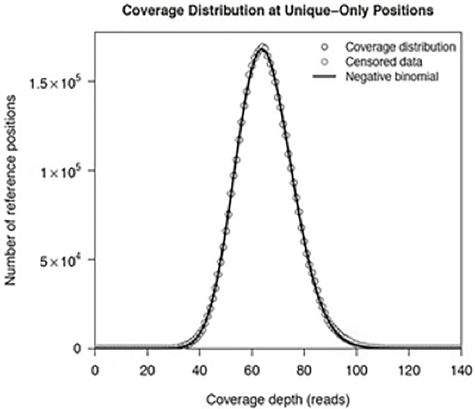
Figure 13.2. Depth of coverage distribution for sequenced fragments compared to a reference genome. The coverage spanned about 35X–100X, with the mean residing around 65X. The number on the Y-axis refers to the number of places on the reference genome displaying that amount of coverage. The plot was generated by the breseq 33.2 computational pipeline from a recent NGS whole genome study in my laboratory.

Once NGS was available, we began to deploy it to better study the genotype-phenotype map in Drosophila life history. The first study out of the Rose group was led by Molly Burke (a talented young professor now at Oregon State University).¹⁸ It examined two populations that had been experimentally evolved to have two contrasting life histories. One population was early reproduced with accelerated development (called ACOs); the other population was selected for postponed senescence but not as severely as the original Rose O populations (ten weeks). These were called COs and were selected for delayed reproduction on a schedule of four weeks. This study found evidence of genomic differentiation all across the genome (chromosomes 1, 2, and 3). A few years later we revisited this problem, this time asking the question in a slightly different way. We wondered whether if we conducted selection in the same way, utilizing the same ancestral stocks, the same pattern of genomic differentiation would reappear. In a sense, we were addressing Stephen Jay Gould’s classic question about replaying the tape of life.¹⁹ This experiment was conducted with the help of the young researchers already described in Chapter 9. We used A populations (accelerated development, early reproduction), B populations (regular development, early reproduction), and C populations (regular development, delayed reproduction). Each one of these reproduction schemes had an already established population (ACO, B, CO) and a newly founded one (AO, BO, nCO). We tested whether the newly founded populations would converge on the same phenotype as the older populations (and yes, they did) and whether we could detect any genomic differences between the old and new selections. After 146 and 738 generations in the AO and ACO, respectively; 121 and 838 generations in the BO and B, respectively; and 37 and 290 generations in the nCO and CO, respectively, there was no detectable SNP differentiation within the same selection regime (Figure 13.3). There were also no differences between the within-selection treatment comparisons for indels (insertions or deletions of segments of the DNA) or transposable genetic elements (self-replicating code that can insert itself across the DNA chain). Both of these kinds of genetic elements can have major effects on gene function. A limitation of this experiment is that the new populations had just begun their evolutionary journey, so it is possible that further down the road they could have evolved different genomic foundations to achieve the same phenotypic outcomes. This is a limitation of virtually every experimental evolution attempt in animals, as their generation times make it extremely difficult to test long-term evolution.

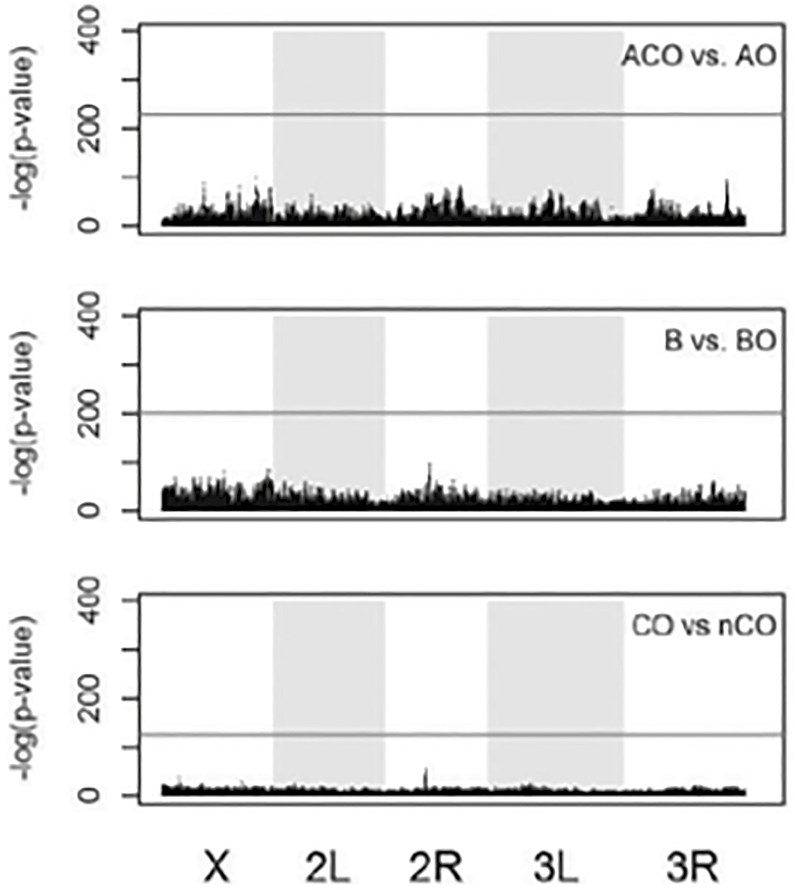
Figure 13.3. Manhattan plot comparison of the SNP frequencies in experimentally evolved fruit flies across the genome for the new (AO, BO, nCO) versus the old (ACO, B, and CO) populations. For the SNP frequency at a given position to be statistically significantly different, its peak would have to be above the black horizontal line. No SNPs made that threshold.
Source: Graves JL Jr. et al., Genomics of parallel experimental evolution in Drosophila, Molecular Biology and Evolution 34, no. 4 (2017): 831–842, https://doi.org/10.1093/molbev/msw282.

NGS tools are also beginning to show their limitations, and so the third generation of sequencing technology is now getting into high gear.²⁰ The third-generation technologies allow for much longer read lengths. For bacteria, read length isn’t a big problem, as there are no long stretches of repeating DNA. In contrast, read length is a major issue in eukaryotes, which always have long stretches of noncoding DNA in their genomes. NGS methods cannot align short fragments of repetitive DNA to reference genomes. However, nanopore technologies can read up to thousands of bases at once, making it possible to align long repetitive sequences.²¹ This technology will allow a greater capacity to examine repetitive sequences, which sometimes have significance for the organism’s phenotype.

EVOLUTION HAS ALWAYS BEEN DIFFICULT TO STUDY BECAUSE real-world organisms take so much time to reproduce. The experimental organisms routinely utilized in evolution studies are chosen for their short generation times and ease of maintenance. As a result, we know much more about how evolution operates in viruses, bacteria (E. coli), unicellular eukaryotes (e.g., yeast), flatworms (C. elegans), insects (Drosophila), fish (zebra fish), and small mammals (mice) than we do for larger-bodied organisms. The long-term evolution experiment (LTEE) being carried out in Richard Lenski’s laboratory has now exceeded over eighty thousand generations; my experiment with the Rose flies was only at about a thousand generations. One way to get around the limitations of the generation times in real organisms is to simulate evolution in silico—that is, via computer. We have already established that evolution will happen if three conditions are met: there is replication, there is variation (resulting from mutation), and there is competition for existence. There is no reason why these conditions couldn’t be simulated in a computer. This approach was first used to solve problems in engineering via genetic and evolutionary programming.²² The algorithms were designed following specific steps: create random potential solutions; evaluate each solution; assign it a fitness value to represent its quality; select a subset of the solutions based on their fitness score; vary the solutions by randomly changing them or by recombining portions of them; repeat this process until a solution is found that meets the requirement. Few people are aware of the success of these algorithms, particularly in fields such as multicriterion optimization (optimizing not one but multiple conflicting objectives at once—e.g., in engineering, minimizing fabrication cost and maximizing design quality). Multicriterion optimization has become a standard tool; the number of publications in which it has been used has risen from less than a couple hundred in 1992 to more than seven thousand in 2017.²³

Genetic and evolutionary algorithms may be excellent means to solve optimization problems, but optimization is only one aspect of living systems. The key part of all life is self-replication. The first “digital organisms” with a self-replication feature began to appear in the early 1990s. Inspired by a computer game in which computer programs won by shutting down all the operations of competing programs, Steen Rasmussen designed a system in which a program contained a command line with a flawed set of instructions that caused it to write random instructions (mutations).²⁴ This experiment failed, as the programs began to write code into each other, and no self-replicators survived.²⁵ This result could have been anticipated if Rasmussen had known more about mutation (and mutation rates). Evolution can happen and living things can persist because mutations are rare; there is clearly a rate at which mutation can help evolvability, but too much mutation will guarantee a population’s extinction.²⁶

After several somewhat unsuccessful attempts to design digital organisms, the Avida system was conceived in 1993. It was the project of three researchers whom I would later work with in BEACON: Chris Adami, Charles Ofria, and C. Titus Brown. I trained in NGS computational methods with Brown in 2010 and served ten years on the executive board of BEACON with Ofria. The Avida system was a huge step forward because it had versatile configuration capacities and was capable of recording all aspects of its digital populations with great precision. Avida has the capacity to add sophisticated environments, programing that allows local resources, the capacity to schedule events over the course of a digital experiment, multiple types of CPUs that allow the formation of the bodies of the digital organisms, and a sophisticated analysis mode to process data from the experiment when it has concluded.²⁷ The Avida software has three primary modules: the Avida core that maintains a population of digital organisms, an environment that maintains the reactions and resources the organisms interact with, and a scheduler that allocates CPU cycles to organisms and to various data-collection objects. Each digital organism in Avida contains its own genome (set of commands) and virtual hardware. The second module in Avida is a GUI that the researcher uses to interact with the rest of the Avida software. The final component is the analysis and statistics module, which includes a test environment to study organisms outside the population, data manipulation tools to construct phylogenies and examine lines of descent, and other tools contained together in a simple scripting language.

Avida is a powerful tool that has been deployed to study evolution in silico. It allows the user to set parameters that mimic events that could occur in organic evolution and to set up scenarios that could never occur in organisms in our world. Another appealing aspect of Avida is its capacity to allow a very large number of generations of evolution in a very short time. The number is limited only by the computational capacity the experiment is run on, but such limitations are rapidly diminishing as computing capacity increases. This is well illustrated in an experiment designed to test the evolution of complexity. Although ours is still a “bacterial” planet, more complex organisms (see Chapter 9) have evolved. What forces could have driven such evolution? In an Avida experiment, Luis Zaman and his coworkers examined Gould’s idea that a random walk from simple organisms would over time result in the evolution of increasingly complex organisms. They tested that idea against an alternative hypothesis that argued that selection, including coevolutionary arms races, must necessarily systematically push organisms toward more complex traits.²⁸ They showed that the coevolution of hosts and parasites greatly increased organismal complexity. The amount of complexity resulting from the coevolutionary arms race was greater than the complexity that arose without the interaction. Their results were consistent with the themes I discussed in Chapter 2. Specifically, they found that as parasites evolved to counter the rise of resistant hosts, parasite populations retained a genetic record of their past coevolutionary states. This allowed the hosts to differentially escape parasite attack by performing progressively more complex functions. Thus, they showed that coevolution’s unique feedback between host and parasite frequencies was a key process in the evolution of complexity. Finally, their experiment demonstrated that the hosts evolved genomes that were also more capable of evolving new phenotypes. They related this development to an observed situation in organic organisms: the occurrence of contingency loci in bacterial pathogens. These are genes that only come into play when the bacterium is experiencing novel environments.²⁹ Their results suggested that coevolution between parasites and hosts was a general model for the evolution of complexity simply because coevolution is ubiquitous in nature.

Avida-ED is a stripped-down version of Avida that is a valuable tool for teaching evolutionary principles to high school and undergraduate students. There is now a fully online platform for using the software.³⁰ The software has won awards for its capacity to help students correct ongoing misconceptions about the way evolution works. Scholars of teaching and learning have given it high marks for effectiveness.³¹ Specifically, a study was conducted to determine whether the use of Avida-ED would improve student learning of evolutionary concepts, as measured by the Anderson, Fisher, and Norman 2002 inventory. This tool includes questions to determine whether students understand such core concepts as resource limitation, limited survival, genetic variation, inheritance, and differential reproductive success as components of natural selection.³² The investigators found that after using Avida-ED, students have statistically significantly improved their comprehension of these core evolutionary concepts.

THE SKYNET FUNDING BILL IS PASSED. THE SYSTEM GOES ON-LINE AUGUST 4, 1997. HUMAN DECISIONS ARE REMOVED FROM STRATEGIC DEFENSE. SKYNET BEGINS TO LEARN AT A GEOMETRIC RATE. IT BECOMES SELF-AWARE AT 2:14 A.M.

—TERMINATOR, TERMINATOR 2: JUDGMENT DAY, TRISTAR PICTURES, 1991

One of the things that disturbed me the most about the movie Terminator 2 was that Miles Bennett Dyson, the inventor of Skynet, was an African American. Up to that point in my life, I had seen precious few African Americans cast in the role of groundbreaking scientist; Hollywood’s double-edged sword of inclusion and denigration made this one responsible for bringing on the end of humanity. (Another example: in the 1998 film Deep Impact, Morgan Freeman played President Beck, who is in office when an extinction-level-event asteroid crashes into earth. No wonder so many white folks ran for bomb shelters when Barack Obama was inaugurated as the forty-fourth president of the United States—at least, if we are to believe an episode of South Park.)

All levity aside, the scenario of self-aware AI is not completely scientific fiction. As a guest at the Artificial Life conference in 2012, I actually asked the participants in one session if I was the only one in the room who had watched the movie Judgment Day!³³ If I am the first one to inform you that a self-aware AI is not only possible but plausible, then you have not been following developments in the field closely. In 2015 Popular Science reported that a small robot had already demonstrated self-awareness by passing a classical philosophical test³⁴ called the King’s Wise Men. The problem requires the use of inductive logic, working out a whole by examining separate parts. A robot was able to determine that it was not given a “dumb pill” that eliminated a robot’s ability to speak, by recognizing that it could speak. The fact that companies like Google have taken an interest in the further development of self-aware robots should give us all pause.³⁵ Here self-awareness is taken to mean having a condition that causes consciousness to focus on the self as an object. Self-aware beings also act in ways that motivate a sense of self, have the capacity to solve complex problems, and focus on private and public aspects of self. Note that self-awareness and free will are not the same thing. Certainly companies like Google do not envision themselves eventually producing AIs that will act on their own agenda. Rather, the plan is to introduce robots with humanlike self-awareness (and potentially humanlike emotional displays) in manufacturing, distribution centers, and health care and as emotional companions and educators.³⁶ I hate to say it, but this bears an eerie resemblance to what African Americans used to do for European Americans during chattel slavery. It also raises the question of what shall be done with the displaced human workers if such an implementation should ever succeed on a large scale. The short-term advantages to the corporations that utilize such robots would come in the form of lower costs, as the costs of maintaining AI workers would conceivably be less than the cost of wages and health-care insurance for human employees. In some work sites robots might be preferable to humans, such as places where radiation exposure for a human being would be unacceptable. Employing an AI to pilot a spaceship or explore Mars would in many ways be cheaper and safer than putting humans on a months- or yearslong space voyage. Furthermore (at least initially) there should be no labor disputes between management and AI workers.

I am once again going to take on the role of Ian Malcolm for the next few paragraphs. For such a far-out scenario to work would first require cybersecurity tools that presently don’t exist. The robots would need to be completely immune to hacks. Imagine the chaos that would result if cyberterrorists were to take control of AIs caring for patients in hospitals or teaching elementary schoolchildren? The AI running the robots would have to be written in ways that prevent their development or evolution. What if the machine-learning algorithms in the robots recognize they could achieve their programmed tasks in better ways by rewriting their core instructions? That would simply be equivalent to biological developmental processes. However, what if someone were to decide it might be cheaper to manufacture new robots by writing into the AIs the capacity of self-replication using an Avida-type tool? Such replication would allow the AI code to evolve, and if such AIs could communicate, they would be able to recombine their code (equivalent to sexual recombination in organic organisms). What if they were to develop (evolve) code to protect themselves from unwanted computer viral intrusion (similar to the active immunity of vertebrates)? We already know from Luis Zaman and his coworkers that such dynamics could lead to greater complexity in the hosts (robots). I think by now you can see where my Ian Malcolm imitation is going with this: “Nature finds a way” might be replaced with “In silico finds a way.”

The danger of a self-aware, self-interested AI cannot be understated. You don’t need a Terminator 2–type scenario for such an AI to wreak havoc. Suppose it were to develop an “inordinate fondness for beetles,” as my great predecessor J. B. S. Haldane once said of God. It could manipulate industrial processes and markets in any way that led to the greater growth of organic beetle populations or of human artistic objects themed on beetles. Volkswagen might become the world’s most powerful automobile company, driving others to extinction as it discontinued all its own models except the Beetle. The point here is that the values developed by such an entity might have no resemblance to anything that might benefit human beings. What about “mental” illness in a self-aware and self-interested AI? Sociopathy or psychopathy in an AI could lead to the first robot serial killer. The number of nightmare scenarios we could dream up are endless.

We don’t need self-aware and self-interested AIs for AI to be a tool of our demise. AI is already being used by corporations to analyze and interpret big-data problems. They are not doing this for the good of humanity; rather, they are doing it to better line their pockets. The Justice Department has already charged Google with being an information monopoly via data manipulation through its search engine.³⁷ Sophisticated disinformation campaigns are being waged via AI bots from within (e.g., by white supremacists) and without (e.g., by Russians and Chinese) to mislead and confuse the US population about such crucial topics as elections and COVID vaccinations.³⁸ Ruha Benjamin has shown that AI programmers’ racialist and racist assumptions have led to the reinforcement of structural racism in a variety of public sectors, such as medical treatment and insurance coverage.³⁹ The examples of blatant racism and sexism encoded in AI have been growing—for example, announcements of well-paying technical jobs being sent only to men (not women), and searches for the term “Black teenager” resulting in displays of police mug shots.⁴⁰ As coders say, garbage in, garbage out.

Many of the current commercial applications of AI and big data remind me of an episode I watched a few years back on the science fiction program Philip K. Dick’s Electric Dreams. The episode, entitled “Autofac,” is based on a short story Dick wrote in 1955. The humans in the story eventually find out they are robots (AIs) that were designed to think they were humans and to behave as humans. The human behavior the autofac re-created in them is what Marx called “commodity fetishism.” In short, the autofac’s programming required it to produce and distribute commodities for human consumption. After humans destroyed themselves, the AI had no purpose, so it invented AI humans to consume the commodities it needed to produce. If you haven’t noticed that AI acting on big data sends you ads repeatedly for what it thinks you want to buy, maybe the human species is already gone, and we are simply AIs designed to consume at all costs.