7
Quantum Mechanics is Incomplete
So We Need to Add Some Things
Statistical Interpretations Based on Local and Crypto Non-local Hidden Variables
Chapters 5 and 6 summarize interpretations of quantum mechanics that follow from the legacy of Copenhagen. They are based on a set of metaphysical preconceptions that tend to side with the anti-realism of Bohr and (especially) Heisenberg, based on the premise that quantum mechanics is complete. In the inaccessible quantum world we’ve finally run up against the boundary between things-in-themselves and things-as-they-appear that philosophers have been warning us about for centuries. We have to come to terms with the fact that there’s nothing to see here, and we’ve reached the end of the road.
But this anti-realist perspective is not to everybody’s taste, as theorist John Bell made all too clear in 1981:1
Making a virtue of necessity, and influenced by positivistic and instrumentalist philosophies, many came to hold not only that it is difficult to find a coherent picture but that it is wrong to look for one—if not actually immoral then certainly unprofessional.
If we make the philosophical choice to side with Einstein, Schrödinger, and Popper and adopt a more realist position, this means we can’t help but indulge our inner metaphysician. We can’t help speculating about a reality beyond the empirical data, a reality lying beneath the things-as-they-appear. We must admit that quantum mechanics is incomplete, and be ready to make frequent visits to the shores of Metaphysical Reality in the hope of finding something—anything—that might help us to complete it.
In doing this we might be led astray, but I honestly think that it goes against the grain of human nature not to try.
Opening the door to realism immediately puts us right back in a fine mess. Any realist interpretation, reformulation, or extension of quantum mechanics necessarily drags along with it all the associated metaphysical preconceptions about how reality ought to be. It must address all the bizarre things that quantum physics appears to allow, such as superpositions now involving real physical states (rather than coded information), the instantaneous collapse of the wavefunction, and the spooky action at a distance this would seem to imply. It has to explain away or eliminate the randomness and discontinuity inherent in quantum mechanics and restore some sense of continuity and cause-and-effect, presided over by a God free of a gambling addiction. It has to find a way to make the quantum world compatible with the classical world, explaining or avoiding an arbitrary ‘shifty split’ between the two.
Where do we start?
In his debate with Bohr and his correspondence with Schrödinger, Einstein had hinted at a statistical interpretation. In his opinion, quantum probabilities, derived as the squares of the wavefunctions,* actually represent statistical probabilities, averaged over large numbers of physically real particles. We resort to probabilities because we’re ignorant of the properties and behaviours of the physically real quantum things. This is very different from anti-realist interpretations which resort to probabilities based on previous experience because we can say nothing meaningful about any of the underlying physics.
Einstein toyed with just such an approach in May 1927. This was a modification of quantum mechanics that combined classical wave and particle descriptions, with the wavefunction taking the role of a ‘guiding field’ (in German, a Führungsfeld), guiding or ‘piloting’ the physically real particles. In this kind of scheme, the wavefunction is responsible for all the wave-like effects, such as diffraction and interference, but the particles maintain their integrity as localized, physically real entities. Instead of waves or particles, as complementarity and the Copenhagen interpretation demands, Einstein’s adaptation of quantum mechanics was constructed from waves and particles.
But Einstein lost his enthusiasm for this approach within a matter of weeks of formulating it. It hadn’t come out as he’d hoped. The wavefunction had taken on a significance much greater than merely statistical. It was almost sinister. Einstein thought the problem was that distant particles were exerting some kind of strange force on one another, which he really didn’t like. But the real problem was that the guiding field is capable of exerting spooky non-local influences—changing something here instantaneously changes some other thing, a long way over there. He withdrew a paper he had written on the approach before it could be published. It survives in the Einstein Archives as a handwritten manuscript.2
We’ll be returning to this kind of ‘pilot-wave’ description in Chapter 8. This experience probably led Einstein to conclude that his initial belief—that quantum mechanics could be completed through a more direct fusion of classical wave and particle concepts—was misguided. He subsequently expressed the opinion that a complete theory could only emerge from a much more radical revision of the entire theoretical structure. Quantum mechanics would eventually be replaced by an elusive grand unified field theory, the search for which took up most of Einstein’s intellectual energy in the last decades of his life.
This early attempt by Einstein at completing quantum mechanics is known generally as a hidden variables formulation, or just a ‘hidden variables theory’. It is based on the idea that there is some aspect of the physics that governs what we see in an experiment, but which makes no appearance in the representation. There are, of course, many precedents for this kind of approach in the history of science. As I’ve already explained, Boltzmann formulated a statistical theory of thermodynamics based on the ‘hidden’ motions of real atoms and molecules. Likewise, in Einstein’s abortive attempt to rethink quantum mechanics, it is the positions and motions of real particles, guided by the wavefunction, that are hidden.
However, in his 1932 book The Mathematical Foundations of Quantum Mechanics, von Neumann presented a proof which appeared to demonstrate that all hidden variable extensions of quantum mechanics are impossible.3 This seemed to be the end of the matter. If hidden variables are impossible, why bother even to speculate about them?
And, indeed, silence prevailed for nearly twenty years. The dogmatic Copenhagen view prevailed, seeping into the mathematical formalism and becoming the quantum physicists’ conscious or unconscious default interpretation. The physics community moved on and just got on with it, content to shut up and calculate.
Then David Bohm broke the silence.
In February 1951, Bohm published a textbook, simply called Quantum Theory, in which he followed the party line and dismissed the challenge posed by EPR’s ‘bolt from the blue’, much as Bohr had done. But even as he was writing the book he was already having misgivings. He felt that something had gone seriously wrong.
Einstein welcomed the book, and invited Bohm to meet with him in Princeton sometime in the spring of 1951. The doubts over the interpretation of quantum theory that had begun to creep into Bohm’s mind now crystallized into a sharply defined problem. ‘This encounter had a strong effect on the direction of my research,’ Bohm later wrote, ‘because I then became seriously interested in whether a deterministic extension of quantum theory could be found.’4 The Copenhagen interpretation had transformed what was really just a method of calculation into an explanation of reality, and Bohm was more committed to the preconceptions of causality and determinism than perhaps he had first thought.
In Quantum Theory, Bohm had asserted that ‘no theory of mechanically determined hidden variables can lead to all of the results of the quantum theory.’5 This was to prove to be a prescient statement. Bohm went on to develop a derivative of the EPR thought experiment which he published in a couple of papers in 1952 and which he elaborated in 1957 with Yakir Aharonov.6 This is based on the idea of fragmenting a diatomic molecule (such as hydrogen, H2) into two atoms.
Now, elementary particles are distinguished not only by their properties of electric charge and mass, but also by a further property which we call spin. This choice of name is a little unfortunate, and arises because some physicists in the 1920s suspected that an electron behaves rather like a little ball of charged matter, spinning around on its axis much like the Earth spins as it orbits the Sun. This is not what happens, but the name stuck.
The quantum phenomenon of spin is indeed associated with a particle’s intrinsic angular momentum, the momentum we associate with rotational motion. Because it also carries electrical charge, a spinning electron behaves like a tiny magnet. But don’t think this happens because the electron really is spinning around its axis. If we really wanted to push this analogy, then we would need to accept that an electron must spin twice around its axis to get back to where it started.* The electron has this property because it is a matter particle called a fermion (named for Enrico Fermi). It has a characteristic spin quantum number of ½ and two spin orientations—two directions the tiny electron magnet can ‘point’ in an external magnetic field. We call these ‘spin up’ (↑) and ‘spin down’ (↓). Sound familiar?
The chemical bond holding the atoms together in a diatomic molecule is formed by overlapping the ‘orbits’ of the electrons of the two atoms and by pairing them so that they have opposite spins—↑↓. In other words, the two electrons in the chemical bond are entangled. Bohm and Aharonov imagined an experiment in which the chemical bond is broken in a way that preserves the spin orientations of the electrons (actually, preserving the electrons’ total angular momentum) in the two atoms. We would then have two atoms—call then atom A and atom B—entangled in spin states ↑ and ↓.
Bohm and Aharonov brought the EPR experiment down from the lofty heights of pure thought and into the practical world of the physics laboratory. In fact, the purpose of their 1957 paper was to claim that experiments capable of measuring correlations between distant entangled particles had already been carried out. For those few physicists paying attention, Bohm’s assertion and the notion of a practical test suggested some mind-blowing possibilities.
John Bell was paying attention. In 1964, he had an insight that was completely to transform questions about the representation of reality at the quantum level. After reviewing and dismissing von Neumann’s ‘impossibility proof’ as flawed and irrelevant, he derived what was to become known as Bell’s inequality. ‘Probably I got that equation into my head and out on to paper within about one weekend,’ he later explained. ‘But in the previous weeks I had been thinking intensely all around these questions. And in the previous years it had been at the back of my head continually.’7
Recall from Chapter 4 that the EPR experiment is based on the creation of a pair of entangled particles, A and B, which we now assume to be atoms. Because the total angular momentum is conserved, we know that the atoms must possess opposite spin-up and spin-down states, which we will continue to write as A↑B↓ and A↓B↑. We assume that the atoms A and B separate as ‘locally real’ particles, meaning that they maintain separate and independent identities and quantum properties as they move apart.
We further assume that making any kind of measurement on A can in no way affect the properties and subsequent behaviour of B. Under these assumptions, when we measure A to be in an ↑ state, we then know with certainty, that B must be in a ↓ state. There is nothing in quantum mechanics that explains how this can happen, the theory is incomplete, and we have a big problem. This is the essence of EPR’s original challenge.
But is any of this really so mysterious? Bell was constantly on the lookout for everyday examples of pairs of objects that are spatially separated but whose properties are correlated, as these provide accessible analogues for the EPR experiment. He found a perfect example in the dress sense of one of his colleagues at CERN, Reinhold Bertlmann. Some years later, Bell wrote:8
The philosopher in the street, who has not suffered a course in quantum mechanics, is quite unimpressed by Einstein–Podolsky–Rosen correlations. He can point to many examples of similar correlations in everyday life. The case of Bertlmann’s socks is often cited. Dr Bertlmann likes to wear two socks of different colours. Which colour he will have on a given foot on a given day is quite unpredictable. But when you see that the first sock is pink you can be already sure that the second sock will not be pink. Observation of the first, and experience of Bertlmann, gives immediate information about the second. There is no accounting for tastes, but apart from that there is no mystery here. And is not this EPR business just the same?
This situation was sketched by Bell himself, and is illustrated in Figure 12.
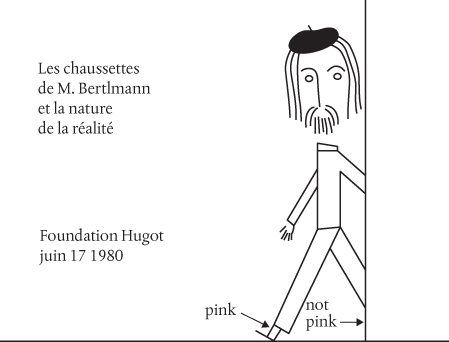
Figure 12 Bertlmann’s socks and the nature of reality.
What if the quantum states of the atoms A and B are fixed by the operation of some local hidden variable at the moment they are formed and, just like Bertlmann’s socks, the atoms move apart in already pre-determined quantum states? This seems to be perfectly logical, and entirely compatible with our first instincts. We can’t deny an element of randomness, just as we can’t deny that Bertlmann may choose at random to wear a pink sock on his left or right foot, so the hidden variable may randomly produce the result A↑B↓ or A↓B↑. But, so long as the spins of atoms A and B are always opposed, it would seem that all is well with the laws of physics.
How would this work? Well, we have no way of knowing what this hidden variable might be or what it might do, but here we are on the shores of Metaphysical Reality where we’re perfectly at liberty to speculate. So, let’s suppose that each atom has a further property we know nothing about, but which we presume acts to pre-determine the spins of A and B in any subsequent measurements. We could think of this property in terms of a tiny pointer, tucked away inside each atom. This can point in any direction in a sphere. When atoms A and B are formed by breaking the bond in the molecule, their respective pointers are firmly fixed in position, but they are constrained by the conservation of angular momentum always to be fixed in opposite directions.
The atoms move apart, the pointers remaining fixed in their positions. Atom A, over on the left, passes between the poles of a magnet, which allows us to measure its spin orientation.* Atom B, on the right, passes between the poles of another magnet, which is aligned in the same direction as the one on the left. We’ll keep this really simple. If the pointer for either A or B is projected anywhere onto the ‘northern’ semicircle, defined in relation to the north pole of its respective magnet (shown as the shaded area in Figure 13), then we measure the atom to be in an ↑ state. If the pointer lies in the ‘southern’ semicircle (the unshaded area), then we measure the atom to be in a ↓ state. Figure 13 shows how a specific (but randomly chosen) orientation of the pointers leads to the measurement outcome A↑B↓.
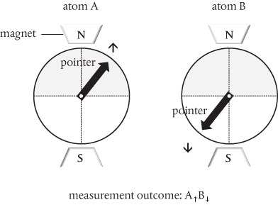
Figure 13 In a simple local hidden variable account of the correlation between the spins of entangled hydrogen atoms, we assume the measurement outcomes are predetermined by a ‘pointer’ in each atom whose direction is fixed at the moment the atoms are formed.
In a sequence of measurements on identically prepared pairs of atoms, we expect to get a random series of results: A↑B↓, A↑B↓, A↓B↑, A↑B↓, A↓B↑, A↓B↑, and so on. If we assume that in each pair the pointer projections can be randomly but uniformly distributed over the entire circle, then in a statistically significant number of measurements we can see that there’s a 50% probability of getting a combined A↑B↓ result.
This is where Bell introduces a whole new level of deviousness. Figure 13 shows an experiment in which the magnets are aligned—the north poles of both magnets lie in the same direction. But what if we now rotate one of the magnets relative to the other? Remember that the ‘northern’ and ‘southern’ semicircles are defined by the orientation of the poles of the magnet. So if the magnet is rotated, so too are the semicircles. But, of course, we’re assuming that the hidden variable pointers themselves are fixed in space at the moment the atoms are formed—the directions in which they point are supposedly determined by the atomic physics and can’t be affected by how we might choose to orientate the magnets in the laboratory. The atoms are assumed to be locally real.
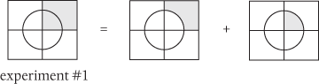
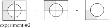
Suppose we conduct a sequence of three experiments:

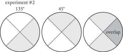
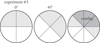
Figure 14 shows how rotating one magnet clockwise relative to the other affects the measurement outcomes for the same pointer directions used in Figure 13. In experiment #1, rotating the magnet for atom B by 135° means that the pointer for B now predetermines an ↑ state, giving the result A↑B↑. This doesn’t mean that we’ve broken any conservation laws—the hidden variable pointers for A and B still point in opposite directions. It just means that we’ve opened up the experiment to a broader range of outcomes: rotating the magnet for atom B means that both A↑B↑ and A↓B↓ results have now become permissible. And, as the probabilities for all the possible results must still sum to 100%, we can see that the probabilities for A↑B↓ and A↓B↑ must therefore fall.

Figure 14 Bell introduced a whole new level of deviousness into the Bohm–Aharanov version of the Einstein–Podolsky–Rosen experiment by rotating the relative orientations of the magnets.
The question I want to ask for each of these experiments is this: What is the probability of getting the outcome A↑B↓? Before rushing to find the answers, I’d like first to establish some numerical relationships between the probabilities for this outcome in each of the experiments. I don’t want to get bogged down here in the maths, so I propose to do this pictorially.9
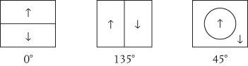
Imagine that we ‘map out’ the individual ↑ and ↓ results—irrespective of whether these relate to A or B—for each orientation of the magnets. For an orientation of 0°, we divide a square into equal upper and lower halves. For 135°, we divide the square into equal left and right halves. We have to be a bit more imaginative for the third 45° orientation, as we have only two dimensions to play with, so we draw a circle inside the square, such that the area of the circle is equal to the area that lies within the square, but outside the circle. This gives us
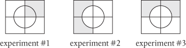
We can now combine these into a single map, which allows us to chart the A↑B↓ results for each of our experiments. For example, in experiment #1, results in which A is measured to be ↑ and B is measured to be ↓ occupy the top right-hand corner of the map, marked below in grey. Likewise for experiments #2 and #3:
We should note once again that this will only work if we can assume that atom A and atom B are entirely separate and distinct, and that making measurements on one can in no way affect the outcomes of measurements on the other. We must assume the atoms to be locally real.
If it helps, think of the grey areas in these diagrams as the places where we would put a tick every time we get an A↑B↓ result in each experiment. We carry out each experiment on exactly the same numbers of pairs of atoms, and we count up how many ticks we have. The number of ticks divided by the total number of pairs we studied then gives us the probability for getting the result A↑B↓ in each experiment.
In fact, these diagrams represent sets of numbers. So let’s have some fun with them. We can write the set for experiment #1 as the sum of two smaller subsets:
Likewise, we can write the set for experiment #2 as
If we now add these two expressions together, we get
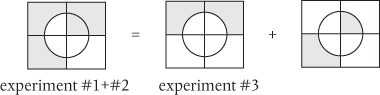
We can’t exclude the possibility that the last subset in this expression won’t have some ticks in it, but I think you’ll agree that it is perfectly safe for us to conclude that
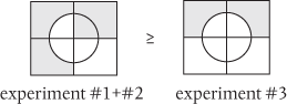
where the symbol ≥ means ‘is greater than or equal to’. This is Bell’s inequality. It actually has nothing whatsoever to do with quantum mechanics or hidden variables. It is simply a logical conclusion derived from the relationships between independent sets of numbers. It is also quite general. It does not depend on what kind of hidden variable theory we might devise, provided this is locally real. This generality allowed Bell to formulate a ‘no-go’ theorem: ‘If the [hidden variable] extension is local it will not agree with quantum mechanics, and if it agrees with quantum mechanics it will not be local.’10 A complementary ‘no-go’ theorem was devised in 1967 by Simon Kochen and Ernst Specker.11
What this form of Bell’s inequality says is that the probability of getting an A↑B↓ result in experiment #1, when added to the probability of getting an A↑B↓ result in experiment #2, must be greater than or at least equal to the probability of getting an A↑B↓ result in experiment #3.
Now, we can deduce these probabilities from our simple local hidden variable theory by examining the overlap between the ‘northern’ semicircles for the two magnets in each experiment, and dividing by 360°. We know from Figure 13 that complete overlap of 180° (the magnets are aligned) means a probability for A↑B↓ of 50%. In experiment #1, the overlap is reduced to 45°, and the probability of getting A↑B↓ falls to 12½%:

In experiment #2, the overlap is 90° (25%):
And in experiment #3 the overlap is 135° (37½%):
These are summarized on the left in the following:
| Probability of getting A↑B↓ local hidden variables | Probability of getting A↑B↓ quantum mechanics | |
|---|---|---|
| Experiment #1 | 12½% | 7.3% |
| Experiment #2 | 25% | 25% |
| Experiment #3 | 37½% | 42.7% |
If we now add the probabilities for #1 and #2 together, then according to a local hidden variables theory we get a total of 37½%, equal to the probability for #3 and therefore entirely consistent with Bell’s inequality.
So, what does quantum mechanics (without hidden variables) predict? I don’t want to go into too much detail here. Trust me when I tell you that the quantum-mechanical prediction for the probability of getting an A↑B↓ result is given by half the square of the cosine of half the angle between the magnets. The quantum-mechanical predictions are summarized in the right-hand column of the table above. If we put these predictions into Bell’s inequality, we get the result that 7.3% + 25% = 32.3% must be greater than or equal to 42.7%.
What we’ve discovered is that quantum mechanics violates Bell’s inequality. It predicts that the extent of the correlation between atoms A and B can sometimes be greater, sometimes less, than any local hidden variable theory can allow.
This is such an important result that it’s worth taking some time to recap, to ensure we understand how we got here. EPR sought to expose the incompleteness of quantum mechanics in a thought experiment involving a pair of entangled particles. If we adopt a realist interpretation of the wavefunction, and we assume that the particles are locally real and measurements on one can’t in any way influence the outcomes of measurements on the other, then something is surely missing. Bohm and Aharonov adapted this experiment and showed how it might provide a practical test. Bell went further, introducing a whole new level of deviousness and devising Bell’s inequality.
Here, indeed, is a direct test: quantum mechanics versus local hidden variables. Which is right? Is Bell’s inequality violated in practice? This is more than enough reason to get back on board the Ship of Science and set sail for Empirical Reality.
Bell wrote his paper in 1964 but, due to a mix-up, it wasn’t published until 1966.12 It took about another ten years for experimental science to develop the degree of sophistication needed to begin to produce some definitive answers.
Although this kind of experimentation continues to this day, perhaps the most famous of these tests was reported in the early 1980s by Alain Aspect and his colleagues at the University of Paris. These were not based on entangled atoms and magnets. Instead they made use of pairs of entangled photons produced in a ‘cascade’ emission from excited calcium atoms.
Like electrons, photons also possess spin angular momentum, but there’s a big difference. Photons are ‘force particles’. They carry the electromagnetic force and are called bosons (named for Satyendra Nath Bose), and have a spin quantum number of 1. Because photons travel at the speed of light, there are only two spin orientations which we associate with left-circularly (⭯) and right-circularly (⭮) polarized light, as judged from the perspective of the source of the light. Now, the outermost electrons in a calcium atom sit in a spherical orbit with their spins paired and zero angular momentum. So, when one of these absorbs a photon and is excited to a higher-energy orbit, it picks up a quantum of angular momentum from the photon. This can’t go into the electron’s spin, since this is fixed. It goes instead into the electron’s orbital motion, pushing it into an orbit with a different shape, from a sphere to a dumbbell—look back at Figure 6c.
But if we now hit the excited calcium atom with another photon, we can excite the electron left behind in the spherical orbit also into the dumbbell-shaped orbit. There are now three possible quantum states, depending on how the spin and orbital angular momenta of the electrons combine together. In one of these the angular momentum cancels to zero.
Although this state is very unstable, the calcium atom can’t simply emit a photon and return to the lowest-energy spherical orbit. This would involve a transition with no change in angular momentum, and there’s simply no photon for that. I suspect you can see where this is going. Instead, the atom emits two photons in rapid succession. One of the photons has a wavelength corresponding to green (we’ll call this photon A) and the other is blue (photon B). As there can be no net change in angular momentum, and angular momentum must be conserved, the photons must be emitted with opposite states of circular polarization.
The photons are entangled.
The advantage of using photon polarization rather than the spin of electrons or atoms is that we can measure the polarization of light in the laboratory quite easily using polarizing analysers, such as calcite crystals.13 We don’t need to use unwieldy magnets.
One small issue. Polarizing analysers don’t measure the circular polarization states of photons; they measure horizontal (↔) or vertical (↕) polarization.* But that’s okay. A left- or right-circularly polarized photon incident on a linear polarizing analyser orientated vertically has a 50% probability of being transmitted. Likewise for an analyser orientated horizontally. And we know well enough by now that a total wavefunction expressed in a basis of left- and right-circular polarization states can be readily changed to a basis of horizontal and vertical polarization states.
Just like Bell’s devious experiment with magnets, the analysers used to measure the polarization states of both photons A and B were mounted on platforms that could be rotated relative to one another. This experiment with entangled photons is entirely equivalent to Bell’s.
One other important point. The detectors for each photon were placed 13 metres apart, on opposite sides of the laboratory. It would take about 40 billionths of a second for any kind of signal travelling at the speed of light to cross this distance. But the experiment was set up to detect pairs of photons A and B arriving within a window of just 20 billionths of a second. In other words, any spooky quantum influences passing between the photons—allowing measurements on one to affect the other—would need to travel faster than the speed of light.
We’re now firmly on the shores of Empirical Reality, and we must acknowledge that the real world can be rather uncooperative. Polarizing analysers ‘leak’, so they don’t provide 100% accuracy. Not all the photons emitted can be ‘gathered’ and channelled into their respective detectors, and the detectors themselves can be quite inefficient, recording only a fraction of the photons that are actually incident on them. Stray photons in the wrong place at the wrong time can lead to miscounting the number of pairs detected.
Some of these very practical deficiencies can be compensated by extending the experiment to a fourth arrangement of the analysers, and writing Bell’s inequality slightly differently. For the particular set of arrangements that Aspect and his colleagues studied, Bell’s inequality places a limit for local hidden variables of less than or equal to 2. Quantum mechanics predicts a maximum of 2 times the square root of 2, or 2.828. Aspect and his colleagues obtained the result 2.697, with an experimental error of ±0.015, a clear violation of Bell’s inequality.14
These results are really quite shocking. They confirm that if we want to interpret the wavefunction realistically, the photons appear to remain mysteriously bound to one another, sharing a single wavefunction, until the moment a measurement is made on one or the other. At this moment the wavefunction collapses and the photons are ‘localized’ in polarization states that are correlated to an extent that simply cannot be accounted for in any theory based on local hidden variables. Measuring the polarization of photon A does seem to affect the result that will be obtained for photon B, and vice versa, even though the photons are so far apart that any communication between them would have to travel faster than the speed of light.
Of course, this was just the beginning. For those physicists with deeply held realist convictions, there just had to be something else going on. More questions were asked: What if the hidden variables are somehow influenced by the way the experiment is set up? This was just the first in a series of ‘loopholes’, invoked in attempts to argue that these results didn’t necessarily rule out all the local hidden variable theories that could possibly be conceived.
Aspect himself had anticipated this first loophole, and performed further experiments to close it off. The experimental arrangement was modified to include devices which could randomly switch the paths of the photons, directing each of them towards analysers orientated at different angles. This prevented the photons from ‘knowing’ in advance along which path they would be travelling, and hence through which analyser they would eventually pass. This is equivalent to changing the relative orientations of the two analysers while the photons were in flight. It made no difference. Bell’s inequality was still violated.15
The problem can’t be made to go away simply by increasing the distance between the source of the entangled particles and the detectors. Experiments have been performed with detectors located in Bellevue and Bernex, two small Swiss villages outside Geneva almost 11 kilometers apart.16 Subsequent experiments placed detectors in La Palma and Tenerife in the Canary Islands, 144 kilometers apart. Bell’s inequality was still violated.17
Okay, but what if the hidden variables are still somehow sensitive even to random choices in the experimental setup, simply because these choices are made on the same timescale? In experiments reported in 2018, the settings were determined by the colours of photons detected from quasars, the active nuclei of distant galaxies. The random choice of settings was therefore already made nearly eight billion years before the experiment was performed, as this is how long it took for the trigger photons to reach the Earth. Bell’s inequality was still violated.18
There are other loopholes, and these too have been closed off in experiments involving both entangled photons and ions (electrically charged atoms). Experiments involving entangled triplets of photons performed in 2000 ruled out all manner of locally realistic hidden variable theories without recourse to Bell’s inequality.19
If we want to adopt a realistic interpretation, then it seems we must accept that this reality is non-local or, at the very least, it violates local causality.
But can we still meet reality halfway? In these experiments, we assume that the properties of the entangled particles are governed by some, possibly very complex, set of hidden variables. These possess unique values that predetermine the quantum states of the particles and their subsequent interactions with the measuring devices. We further assume that the particles are formed with a statistical distribution of these variables determined only by the physics and not by the way the experiment is set up.
Local hidden variable theories are characterized by two further assumptions. In the first, we assume (as did EPR) that the outcome of the measurement on particle A can in no way affect the outcome of the measurement on B, and vice versa. In the second, we assume that the setting of the device we use to make the measurement on A can in no way affect the outcome of the measurement on B, and vice versa.
The experimental violation of Bell’s inequality shows that one or other (or both) of these assumptions is invalid. But, of course, these experiments don’t tell us which.
In a paper published in 2003, Nobel laureate Anthony Leggett chose to drop the setting assumption. This admits that the behaviour of the particles and the outcomes of subsequent measurements is influenced by the way the measuring devices are set up. This is still all very spooky and highly counterintuitive:20
nothing in our experience of physics indicates that the orientation of distant [measuring devices] is either more or less likely to affect the outcome of an experiment than, say, the position of the keys in the experimenter’s pocket or the time shown by the clock on the wall.
By keeping the outcome assumption, we define a class of non-local hidden variable theories in which the individual particles possess defined properties before the act of measurement. What is actually measured will of course depend on the settings, and changing these settings will somehow affect the behaviour of distant particles (hence, ‘non-local’). Leggett referred to this broad class of theories as ‘crypto’ non-local hidden variable theories. They represent a kind of halfway house between strictly local and completely non-local.
He went on to show that dropping the setting assumption is in itself still insufficient to reproduce all the results of quantum mechanics. Just as Bell had done in 1964, he derived an inequality that is valid for all classes of crypto non-local hidden variable theories but which is predicted to be violated by quantum mechanics. At stake then was the rather simple question of whether quantum particles have the properties we assign to them before the act of measurement. Put another way, here was an opportunity to test whether quantum particles have what we might want to consider as ‘real’ properties before they are measured.
The results of experiments designed to test Leggett’s inequality were reported in 2007 and, once again, the answer is pretty unequivocal. For a specific arrangement of the settings in these experiments, Leggett’s inequality demands a result which is less than or equal to 3.779. Quantum mechanics predicts 3.879, a violation of less than 3%. The experimental result was 3.8521, with an error of ±0.0227. Leggett’s inequality was violated.21 Several variations of experiments to test Leggett’s inequality have been performed more recently. All confirm this general result.
It would seem that there is no grand conspiracy of nature that can be devised which will preserve locality. In 2011, Mathew Pusey, Jonathan Barrett, and Terry Rudolph at Imperial College in London published another ‘no-go’ theorem.22 In essence, this says that any kind of hidden variable extension in which the wavefunction is interpreted purely statistically cannot reproduce all the predictions of quantum mechanics.
The ‘PBR theorem’, as it is called, sparked some confusion and a lot of debate when it was first published.23 It was positioned as a theorem which rules out all manner of interpretations in which the wavefunction represents ‘knowledge’ in favour of interpretations in which the wavefunction is considered to be real. But ‘knowledge’ here is qualified as knowledge derived from the statistics of whatever it is that is assumed to underlie the physics and which is further assumed to be objectively real. Whilst it rules in favour of realist interpretations that are not based on statistics, it does not rule out the kinds of anti-realist interpretations which we considered in Chapters 5 and 6.
We should note in passing that whilst local or crypto non-local hidden variable theories have been all but ruled out by these experiments, they underline quite powerfully how realistic interpretations have provided compelling reasons for the experimentalists to roll up their sleeves and get involved. In this case, the search for theoretical insight and understanding, in the spirit of Proposition #4 (see the Appendix), has encouraged some truly wonderful experimental innovations. The relatively new scientific disciplines of quantum information, quantum computing, and quantum cryptography have derived in part from efforts to resolve these foundational questions and to explore the curious phenomenon of entanglement, even though the search for meaningful answers has so far proved fruitless.
But we must now confront the conclusion from all the experimental tests of Bell’s and of Leggett’s inequalities. In any realistic interpretation in which the wavefunction is assumed to represent the real physical state of a quantum system, the wavefunction must be non-local or it must violate local causality.
Okay, so let’s see what that means.