10.6. Thwaites’ Method
To solve (10.43) at least two additional equations are needed. Using the correlation parameter:
 (10.44)
introduced by Holstein and Bohlen (1940), Thwaites (1949) developed an approximate solution to (10.43) that involves two empirical dimensionless functions l(λ) and H(λ):
 (10.45, 10.46)
that are listed in Table 10.2. This tabulation is identical to Thwaites' original for λ ≥ –0.060 but includes the improvements recommended by Curle and Skan a few years later (see Curle, 1962) for λ < –0.060. The function l(λ) is sometimes known as the shear correlation while H(λ) is commonly called the shape factor.
 (10.47)
The definitions of l and H allow the second version to be simplified:

The momentum thickness θ can be eliminated from this equation using (10.44), to find:
 (10.48)
Fortunately, L(λ) ≈ 0.45 – 6.0λ = 0.45 + 6.0m, is approximately linear as shown in Figure 10.9 which is taken from Thwaites’ (1949) original paper where m = –λ. With this linear fit, (10.48) can be integrated:
 (10.49)
The second version of (10.49) is a first-order linear inhomogeneous differential equation for θ2/ν, and its integrating factor is U e 6  . The resulting solution for θ2 involves a simple integral of the fifth power of the free-stream velocity at the edge of the boundary layer:
. The resulting solution for θ2 involves a simple integral of the fifth power of the free-stream velocity at the edge of the boundary layer: (10.50)
where x′ is an integration variable, and θ = θ0 and Ue = U0 at x = 0. If x = 0 is a stagnation point (Ue = 0), then it is safe to set θ0 = 0 since the exterior flow must accelerate away from a stagnation point and accelerating external flow leads to boundary-layer initial-condition memory loss. Once the integration specified by (10.50) is complete, the surface shear stress and displacement thickness can be recovered by computing λ and then using (10.45), (10.46), and Table 10.2.
Overall, the accuracy of Thwaites’ method is ±3% or so for favorable pressure gradients, and ±10% for adverse pressure gradients but perhaps slightly worse near boundary-layer separation. The great strength of Thwaites’ method is that it involves only one parameter (λ) and requires only a single integration. This simplicity makes it ideal for preliminary engineering calculations that are likely to be followed by more formal computations or experiments.
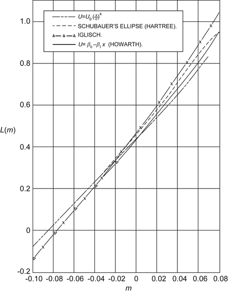
Figure 10.9 Plot of L(m) from (10.48) vs. m = –λ from Thwaites' 1949 paper. Here a suitable empirical fit to the four sources of laminar boundary-layer data is provided by L(m) = 0.45 + 6.0m = 0.45 – 6.0λ. Reprinted with the permission of The Royal Aeronautical Society.
Table 10.2
Universal Functions for Thwaites’ Method
| λ | l(λ) | H(λ) |
| 0.25 | 0.500 | 2.00 |
| 0.20 | 0.463 | 2.07 |
| 0.14 | 0.404 | 2.18 |
| 0.12 | 0.382 | 2.23 |
| 0.10 | 0.359 | 2.28 |
| 0.08 | 0.333 | 2.34 |
| 0.064 | 0.313 | 2.39 |
| 0.048 | 0.291 | 2.44 |
| 0.032 | 0.268 | 2.49 |
| 0.016 | 0.244 | 2.55 |
| 0.0 | 0.220 | 2.61 |
| –0.008 | 0.208 | 2.64 |
| –0.016 | 0.195 | 2.67 |
| –0.024 | 0.182 | 2.71 |
| –0.032 | 0.168 | 2.75 |
| –0.040 | 0.153 | 2.81 |
| –0.048 | 0.138 | 2.87 |
| –0.052 | 0.130 | 2.90 |
| –0.056 | 0.122 | 2.94 |
| –0.060 | 0.113 | 2.99 |
| –0.064 | 0.104 | 3.04 |
| –0.068 | 0.095 | 3.09 |
| –0.072 | 0.085 | 3.15 |
| –0.076 | 0.072 | 3.22 |
| –0.080 | 0.056 | 3.30 |
| –0.084 | 0.038 | 3.39 |
| –0.086 | 0.027 | 3.44 |
| –0.088 | 0.015 | 3.49 |
| –0.090 | 0.0 | 3.55 |
Before proceeding to example calculations, an important limitation of boundary-layer calculations that start from a steady presumed surface pressure distribution (such as Thwaites’ method) must be stated. Such techniques can only predict the existence of boundary-layer separation; they do not reliably predict the location of boundary-layer separation. As will be further discussed in the next section, once a boundary layer separates from the surface on which it has formed, the fluid mechanics of the situation are entirely changed. First of all, the boundary-layer approximation is invalid downstream of the separation point because the layer is no longer thin and contiguous to the surface; thus, the scaling (10.6) is no longer valid. Second, separation commonly leads to unsteadiness because separated boundary layers are unstable and may produce fluctuations even if all boundary conditions are steady. And third, a separated boundary layer commonly has an enormous flow-displacement effect that drastically changes the outer flow so that it no longer imposes the presumed attached boundary-layer surface pressure distribution. Thus, any boundary-layer calculation that starts from a presumed surface pressure distribution should be abandoned once that calculation predicts the occurrence of boundary-layer separation.
The following two examples illustrate the use of Thwaites’ method with and without a prediction of the occurrence of boundary-layer separation.
Example 10.6
Use Thwaites' method to estimate the momentum thickness, displacement thickness, and wall shear stress of the Blasius boundary layer with θ0 = 0 at x = 0.
Solution
The solution plan is to use (10.50) to obtain θ. Then, because dUe/dx = 0 for the Blasius boundary layer, λ = 0 at all downstream locations and the remaining boundary-layer parameters can be determined from the θ results, (10.45), (10.46), and Table 10.2. The first step is setting Ue = U = constant in (10.50) with θ0 = 0:

This approximate answer is 1% higher than the Blasius-solution value. For λ = 0, the tabulated shape factor is H(0) = 2.61, so:
This approximate answer is also 1% higher than the Blasius-solution value. For λ = 0, the shear correlation value is l(0) = 0.220, so:
which implies a skin friction coefficient of:
which is 1.2% below the Blasius-solution value.
Example 10.7
A shallow-angle, two-dimensional diffuser of length L is designed for installation downstream of a blower in a ventilation system to slow the blower-outlet airflow via an increase in duct cross-sectional area (see Figure 10.10). If the diffuser should reduce the flow speed by half by doubling the flow area and the boundary layer is laminar, is boundary-layer separation likely to occur in this diffuser?
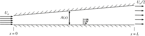
Figure 10.10 A simple two-dimensional diffuser of length L intended to slow the incoming flow to half its speed by doubling the flow area. The resulting adverse pressure gradient in the diffuser influences the character of the boundary layers that develop on the diffuser's inner surfaces, especially when these boundary layers are laminar.
Solution
The first step is to determine the outer flow Ue(x) by assuming uniform (ideal) flow within the diffuser. Then, (10.50) can be used to estimate θ2(x) and λ(x). Boundary-layer separation will occur if λ falls below –0.090.
For uniform incompressible flow within the diffuser: U1A1 = Ue(x)A(x), where (1) denotes the diffuser inlet, Ue(x) is the flow speed, A(x) is the diffuser's cross sectional area. For flat diffuser sides, a doubling of the flow area in a distance L, requires A(x) = A1(1 + x/L), so the ideal outer flow velocity is Ue(x) = U1(1 + x/L)–1. With this exterior velocity the Thwaites' integral becomes:
where U0 = U1 in this case. The 0-to-x integration is readily completed and this produces:
From this equation it is clear that θ grows with increasing x. This relationship can be converted to λ by multiplying it with (1/ν)dUe/dx = – (U1/νL)(1 + x/L)–2:
In this case, even when θ0 = 0, λ will (at best) start at zero and become increasingly negative with increasing x. At this point, a determination of whether or not boundary-layer separation will occur involves calculating λ as function of x/L. The following table comes from evaluating the last equation with θ0 = 0.
Here, Thwaites' method predicts that boundary-layer separation will occur, since λ will fall below –0.090 at x/L ≈ 0.16, a location that is far short of the end of the diffuser at x = L. While it is tempting to consider this a prediction of the location of boundary-layer separation, such a temptation should be avoided. In addition, if θ0 was non-zero, then λ would decrease even more quickly than shown in the table, making the positive prediction of boundary-layer separation even firmer. Thus, successful prediction of the flow in this diffuser requires simultaneous assessment of the whole flow field. Partitioning the equation-solving effort into an ideal outer flow and a steady laminar inner flow is not successful in this case. (In reality, diffusers in duct work and flow systems are common but they typically operate with turbulent boundary layers that more effectively resist separation.)