Chapter 10
Boundary Layers and Related Topics
Abstract
Laminar boundary-layer flows occur when a moving viscous fluid comes in contact with a solid surface and a layer of rotational fluid, the boundary layer, forms in response to the action of viscosity and the no-slip boundary condition on the surface. When the surface is flat or mildly curved and the boundary layer that develops on it is thin and remains adjacent to it, the flow within this layer may be determined by simplifying the Navier-Stokes equations to account for the flow's geometry and then solving the simplified equations. Unfortunately, when the pressure increases in the downstream direction or when the surface is highly curved, the boundary layer may leave the surface, a phenomenon known as separation, and the simplified form of the Navier-Stokes equations no longer applies. In addition, at sufficiently high Reynolds number, boundary-layer flows may spontaneously become unsteady and then transition to turbulence. In combination, these phenomena provide explanations for the fluid dynamic forces felt as fluid moves past a cylinder or sphere at different Reynolds numbers.
Keywords
Boundary-layer approximation; Laminar flow; Boundary-layer thickness; Blasius solution; Falkner-Skan solutions; Thwaites’ method; Transition; Separation; Flow past a cylinder; Flow past a sphere; Bluff body flow• To describe the boundary-layer concept and the mathematical simplifications it allows in the complete equations of motion for a viscous fluid
• To present the equations of fluid motion for attached laminar boundary layers
• To provide a variety of exact and approximate steady laminar boundary-layer solutions
• To discuss the Reynolds number dependent phenomena associated with flow past bluff bodies
• To illustrate the use of a boundary-layer solution methodology for free and wall-bounded jet flows
10.1. Introduction
Until the beginning of the twentieth century, analytical solutions of steady fluid flows were generally known for two typical situations. One of these was that of parallel viscous flows and low Reynolds number flows, in which the nonlinear advective terms were zero (or very small), and pressure and viscous forces balanced. The second type of solution was that of inviscid flows around bodies of various shapes, in which inertia and pressure forces balanced. Although the equations of motion are nonlinear in this second situation, the velocity field can be determined by solving the linear Laplace equation. These irrotational solutions predicted pressure forces on a streamlined body that agreed surprisingly well with experimental data for flow of fluids of small viscosity. However, these solutions also predicted zero drag force and a non-zero tangential velocity at the body surface, features that did not agree with the experiments.
In 1905 Ludwig Prandtl, an engineer by profession and therefore motivated to find realistic fields near bodies of various shapes, first hypothesized that, for small viscosity, the viscous forces are negligible everywhere except close to solid boundaries where the no-slip condition had to be satisfied. The thickness of these boundary layers approaches zero as the viscosity goes to zero. Prandtl’s hypothesis reconciled two rather contradictory facts. It supported the intuitive idea that the effects of viscosity are indeed negligible in most of the flow field if ν is small, but it also accounted for drag by insisting that the no-slip condition must be satisfied at a solid surface, no matter how small the viscosity. This reconciliation was Prandtl’s aim, which he achieved brilliantly. Prandtl also showed how the full equations of fluid motion within the boundary layer can be simplified. Since the time of Prandtl, the concept of the boundary layer has been generalized, and the mathematical techniques involved have been formalized, extended, and applied in other branches of physical science (see van Dyke, 1975; Bender & Orszag, 1978; Kevorkian & Cole 1981; Nayfeh, 1981). The boundary-layer concept is considered a cornerstone in the intellectual foundation of fluid mechanics.
This chapter presents the boundary-layer hypothesis and examines its consequences. The equations of fluid motion within the boundary layer can be simplified because of the layer’s thinness, and exact or approximate solutions can be obtained in many cases. In addition, boundary-layer phenomena provide explanations for the lift and drag characteristics of bodies of various shapes in high Reynolds number flows, including turbulent flows. In particular, the fluid mechanics of curved sports-ball trajectories is described here.
The fundamental assumption of boundary-layer theory is that the layer is thin compared to other length scales such as the length or radius of curvature of the surface on which the boundary layer develops. Across this thin layer, which can exist only in high Reynolds number flows, the velocity varies rapidly enough for viscous effects to be important. This is depicted in Figure 10.1, where the boundary-layer thickness is greatly exaggerated. (On a typical airplane wing, which may have a chord of several meters, the boundary-layer thickness is of order one centimeter.) However, thin viscous layers exist not only next to solid walls but also in the form of jets, wakes, and shear layers if the Reynolds number is sufficiently high. So, to be specific, we shall first consider the boundary layer contiguous to a solid surface, adopting a curving coordinate system that conforms to the surface where x increases along the surface and y increases normal to it. Here the surface may be curved but its radius of curvature is assumed to be much larger than the boundary-layer thickness. We shall refer to the solution of the irrotational flow outside the boundary layer as the outer problem and that of the boundary-layer flow as the inner problem.
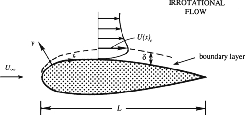
Figure 10.1 A boundary layer forms when a viscous fluid moves over a solid surface. Only the boundary layer on the top surface of the foil is depicted in the figure and its thickness, δ, is greatly exaggerated. Here, U∞ is the oncoming free-stream velocity and Ue is the velocity at the edge of the boundary layer. The usual boundary layer coordinate system allows the x-axis to coincide with a mildly curved surface so that the y-axis lies in the surface-normal direction.
For a thin boundary layer that is contiguous to the solid surface on which it has formed, the full equations of motion for a constant-density constant-viscosity fluid, (4.10) and (9.1), may be simplified. Let δ ¯ ( x )  be the average thickness of the boundary layer at downstream location x on the surface of a body having a local radius of curvature R. The steady-flow momentum equation for the surface-parallel velocity component, u, is:
be the average thickness of the boundary layer at downstream location x on the surface of a body having a local radius of curvature R. The steady-flow momentum equation for the surface-parallel velocity component, u, is: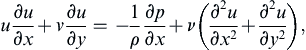 (10.1)
which is valid when δ ¯ / R ≪ 1  . The more general curvilinear form for arbitrary R(x) is given in Goldstein (1938) and Schlichting (1979), but the essential features of viscous boundary layers can be illustrated via (10.1) without additional complications.
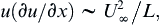
. The more general curvilinear form for arbitrary R(x) is given in Goldstein (1938) and Schlichting (1979), but the essential features of viscous boundary layers can be illustrated via (10.1) without additional complications.Let the characteristic magnitude of u be U∞, the velocity at a large distance upstream of the body, and let L be the stream-wise distance over which u changes appreciably. The longitudinal length of the body can serve as L, because u within the boundary layer may change in the stream-wise direction by a large fraction of U∞ over a distance L (Figure 10.2). A measure of ∂u/∂x is therefore U∞/L, so that the approximate size of the first advective term in (9.1) is:
 (10.2)
where ∼ is to be interpreted as “of order.” We shall see shortly that the other advective term in (10.1) is of the same order. The approximate size of the viscous stress term in (10.1) is:
 (10.3)
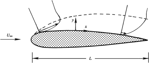
Figure 10.2 Velocity profiles at two positions within the boundary layer. Here again, the boundary-layer thickness is greatly exaggerated. The two velocity vectors are drawn at the same distance y from the surface, showing that the variation of u over a distance x ∼ L is of the order of the free-stream velocity U∞.
The magnitude of δ ¯  can now be estimated by noting that the advective and viscous terms should be of the same order within the boundary layer. Equating the magnitudes of advective and viscous terms in (10.2) and (10.3) leads to:
can now be estimated by noting that the advective and viscous terms should be of the same order within the boundary layer. Equating the magnitudes of advective and viscous terms in (10.2) and (10.3) leads to: (10.4)
This estimate of δ ¯
can also be obtained by noting that viscous effects diffuse to a distance of order [νt]1/2 in time t and that the time-of-flight for a fluid element along a body of length L is of order L/U∞. Substituting L/U∞ for t in [νt]1/2 suggests the viscous layer's diffusive thickness at x = L is of order [νL/U∞]1/2, which is the duplicates (10.4).A formal simplification of the equations of motion within the boundary layer can now be performed. The basic idea is that variations across the boundary layer occur over a much shorter length scale than variations along the layer, that is:
 (10.5)
where δ ¯ v / δ ¯  , so the proper velocity scale for v is
 δ ¯ U ∞ / L = U ∞ Re − 1 / 2 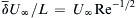 . At high Re, experimental data show that the pressure distribution on the body is nearly that in an irrotational flow over the body, implying that the pressure variations scale with the fluid inertia:
 p − p ∞ ∼ ρ U ∞ 2  . Thus, the proper dimensionless variables for boundary-layer flow are:
≪ L when Re ≫ 1 from (10.4). When applied to the continuity equation, ∂u/∂x + ∂v/∂y = 0, this derivative scaling requires U∞/L ∼ , so the proper velocity scale for v is . At high Re, experimental data show that the pressure distribution on the body is nearly that in an irrotational flow over the body, implying that the pressure variations scale with the fluid inertia: . Thus, the proper dimensionless variables for boundary-layer flow are: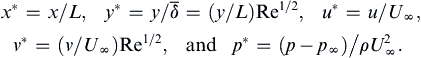 (10.6)
For the coordinates and the velocities, this scaling is similar to that of (9.14) with ε = Re–1/2. The primary effect of (10.6) is a magnification of the surface-normal coordinate y and velocity v by a factor of Re1/2 compared to the stream-wise coordinate x and velocity u. In terms of these dimensionless variables, the steady two-dimensional equations of motion are:
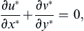 (9.15)
 (10.7)
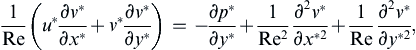 (10.8)
where Re ≡ U∞L/ν is an overall Reynolds number. In these equations, each of the dimensionless variables and their derivatives should be of order unity when the scaling assumptions embodied in (10.6) are valid. Thus, it follows that the importance of each term in (9.15), (10.7), and (10.8) is determined by its coefficient. So, as Re → ∞, the terms with coefficients of 1/Re or 1/Re2 drop out asymptotically. Thus, the relevant equations for laminar boundary-layer flow, in dimensional form, are:
 (7.2, 10.9, 10.10)
This scaling exercise has shown which terms must be kept and which terms may be dropped under the boundary-layer assumption. It differs from the scalings that produced (4.10) and (9.47) because the x and y directions are scaled differently in (10.6) which causes a second derivative term to be retained in (10.9).
Equation (10.10) implies that the pressure is approximately uniform through the thickness of the boundary layer, an important result. The pressure at the surface is therefore equal to that at the edge of the boundary layer, so it can be found from an ideal outer-flow solution for flow above the surface. Thus, the outer flow imposes the pressure on the boundary layer. This justifies the experimental fact that the observed surface pressures underneath attached boundary layers are approximately equal to that calculated from the ideal flow theory. A vanishing ∂p/∂y, however, is not valid if the boundary layer separates from the surface or if the radius of curvature of the surface is not large compared with the boundary-layer thickness.
Although the steady boundary-layer equations (7.2), (10.9), and (10.10) do represent a significant simplification of the full equations, they are still nonlinear second-order partial differential equations that can only be solved when appropriate boundary and matching conditions are specified. If the exterior flow is presumed to be known and irrotational (and the fluid density is constant), the pressure gradient at the edge of the boundary layer can be found by differentiating the steady constant-density Bernoulli equation (without the body force term), p + 1 2 ρ U e 2 = const . 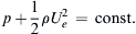 , to find:
, to find: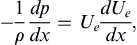 (10.11)
where Ue(x) is the velocity at the edge of the boundary layer. Equation (10.11) represents a matching condition between the outer ideal-flow solution and the inner boundary-layer solution in the region where both solutions must be valid. The (usual) remaining boundary conditions on the fluid velocities of the inner solution are:
 (10.12a,b)
 (10.13)
 (10.14)
For two-dimensional flow, (7.2), (10.9), and the conditions (10.11) through (10.14), completely specify the inner solution as long as the boundary layer remains thin and contiguous to the surface on which it develops. Condition (10.13) merely means that the boundary layer must join smoothly with the outer flow; for the inner solution, points outside the boundary layer are represented by y→∞, although we mean this strictly in terms of the dimensionless distance y / δ ¯  = (y/L)Re1/2→∞. Condition (10.14) implies that an initial velocity profile uin(y) at some location x0 is required for solving the problem. Such a condition is needed because the terms u∂u/∂x and ν∂2u/∂y2 give the boundary-layer equations a parabolic character, with x playing the role of a time-like variable. Recall the Stokes problem of a suddenly accelerated plate, discussed in the preceding chapter, where the simplified field equation is ∂u/∂t = ν∂2u/∂y2. In such problems governed by parabolic equations, the field at a certain time or place depends only on its past or upstream history. Boundary layers therefore transfer viscous effects only in the downstream direction. In contrast, the complete Navier-Stokes equations are elliptic and thus require boundary conditions on the velocity (or its derivative normal to the boundary) upstream, downstream, and on the top and bottom boundaries, that is, all around. (The upstream influence of the downstream boundary condition is a common concern in fluid dynamic computations).
= (y/L)Re1/2→∞. Condition (10.14) implies that an initial velocity profile uin(y) at some location x0 is required for solving the problem. Such a condition is needed because the terms u∂u/∂x and ν∂2u/∂y2 give the boundary-layer equations a parabolic character, with x playing the role of a time-like variable. Recall the Stokes problem of a suddenly accelerated plate, discussed in the preceding chapter, where the simplified field equation is ∂u/∂t = ν∂2u/∂y2. In such problems governed by parabolic equations, the field at a certain time or place depends only on its past or upstream history. Boundary layers therefore transfer viscous effects only in the downstream direction. In contrast, the complete Navier-Stokes equations are elliptic and thus require boundary conditions on the velocity (or its derivative normal to the boundary) upstream, downstream, and on the top and bottom boundaries, that is, all around. (The upstream influence of the downstream boundary condition is a common concern in fluid dynamic computations).Considering two dimensions, an ideal outer flow solution from (7.5) or (7.12) and (7.18), and a viscous inner flow solution as described here would seem to fully solve the problem of uniform flow of a viscous fluid past a solid object. The solution procedure could be a two-step process. First, the outer flow is determined, neglecting the existence of the boundary layer, an error that gets smaller when the boundary layer becomes thinner. Then, (10.11) could be used to determine the surface pressure, and (7.2) and (10.9) could be solved for the boundary-layer flow using the surface-pressure gradient determined from the outer flow solution. If necessary this process might even be iterated to achieve higher accuracy by re-solving for the outer flow with the first-pass-solution boundary-layer characteristics included, and then proceeding to a second solution of the boundary-layer equations using the corrected outer-flow solution. In practice, such an approach can be successful and it converges when the boundary layer stays thin and attached. However, it does not converge when the boundary layer thickens or departs (separates) from the surface on which it has developed. Boundary-layer separation occurs when the surface shear stress, τw, produced by the boundary layer vanishes and reverse (or upstream-directed) flow occurs near the surface. Boundary-layer separation is discussed further in Sections 10.6–10.7. Here it is sufficient to point out that ideal flow around non-slender or bluff bodies typically produces surface pressure gradients that lead to boundary-layer separation.
In summary, the simplifications of the boundary-layer assumption are as follows. First, diffusion in the stream-wise direction is negligible compared to that in the wall normal direction. Second, the pressure in the boundary layer can be found from the outer flow, so that it is regarded as a known quantity within the boundary layer that does not vary perpendicular to the surface. Furthermore, a crude estimate of τw, the wall shear stress, can be made from the various scalings employed earlier: τ w ∼ μ U / δ ¯ ∼ ( μ U / L ) Re 1 / 2 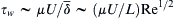 . This implies a skin friction coefficient of:
. This implies a skin friction coefficient of: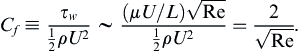 (10.15)
The skin friction coefficient is an important dimensionless parameter in boundary-layer flows. It specifies the fraction of the local dynamic pressure, 1 2 ρ U 2  , that is felt as shear stress on the surface. Here for laminar boundary layers, (10.15) provides the correct order of magnitude and parametric dependence on Reynolds number. However, the numerical factor differs for different laminar boundary-layer flows.
, that is felt as shear stress on the surface. Here for laminar boundary layers, (10.15) provides the correct order of magnitude and parametric dependence on Reynolds number. However, the numerical factor differs for different laminar boundary-layer flows.Example 10.1
For time-averaged turbulent boundary-layer flow, the advective acceleration scaling (10.2) is still appropriate. However, the laminar shear stress relationship (10.3) should be replaced with ∂ τ / ∂ y ∼ τ w / δ ¯  . What is the scaling for the skin friction coefficient in this case?
. What is the scaling for the skin friction coefficient in this case?Solution
As was done to reach (10.4), equate the advective and shear-stress accelerations:

where the second scaling follows from (10.15), the definition of the skin friction. Canceling common terms between the two ends of this relationship then produces:

Although the Reynolds number dependence of Cf is not revealed by this simple relationship, it does suggest Cf will be much less than unity for attached turbulent boundary-layer flows. Measurements in flat-plate turbulent boundary-layer flows on smooth walls typically produce Cf ∼ 0.001 to 0.004 with the lower values occurring at higher Reynolds number; see Section 10.7.