4.11. Dimensionless Forms of the Equations and Dynamic Similarity
For a properly specified fluid flow problem or situation, the differential equations of fluid motion, the fluid’s constitutive and thermodynamic properties, and the boundary conditions may be used to determine the dimensionless parameters that govern the situation of interest even before a solution of the equations is attempted. The dimensionless parameters so determined set the importance of the various terms in the governing differential equations, and thereby indicate which phenomena will be important in the resulting flow. This section describes and presents the primary dimensionless parameters or numbers required in the remainder of the text. Many others not mentioned here are defined and used in the broad realm of fluid mechanics.
The dimensionless parameters for any particular problem can be determined in two ways. They can be deduced directly from the governing differential equations if these equations are known; this method is illustrated here. However, if the governing differential equations are unknown or the parameter of interest does not appear in the known equations, dimensionless parameters can be determined from dimensional analysis (see Section 1.11). The advantage of adopting the former strategy is that dimensionless parameters determined from the equations of motion are more readily interpreted and linked to the physical phenomena occurring in the flow. Thus, knowledge of the relevant dimensionless parameters frequently aids the solution process, especially when assumptions and approximations are necessary to reach a solution.
In addition, the dimensionless parameters obtained from the equations of fluid motion set the conditions under which scale model testing will prove useful for predicting the performance of smaller or larger devices. In particular, two flow fields are considered to be dynamically similar when: (1) their geometries are scale similar, and (2) their dimensionless parameters match. The first requirement implies that any length scale in the first flow field may be mapped to its counterpart in the second flow field by multiplication with a single scale ratio. The second requirement allows predictions for the larger- or smaller-scale flow to be made from quantitative knowledge of the model scale flow when the scale ratio is accounted for. Moreover, use of standard dimensionless parameters typically reduces the parameters that must be varied in an experiment or calculation, and greatly facilitates the comparison of measured or computed results with prior work conducted under potentially different conditions.
To illustrate these advantages, consider the drag force FD on a sphere, of diameter d moving at a speed U through a fluid of density ρ and viscosity μ. Dimensional analysis (Section 1.11) using these five parameters produces the following possible dimensionless scaling laws:
 (4.99)
Both are valid, but the first is preferred because it contains dimensionless groups that either come from the equations of motion or are traditionally defined in the study of fluid dynamic drag. If dimensionless groups were not used, experiments would have to be conducted to determine FD as a function of d, keeping U, ρ, and μ fixed. Then, experiments would have to be conducted to determine FD as a function of U, keeping d, ρ, and μ fixed, and so on. However, such a duplication of effort is unnecessary when dimensionless groups are used. In fact, use of the first dimensionless law above allows experimental results from a wide range of conditions to be simply plotted with two axes (see Figure 4.23) even though the full complement of experiments may have involved variations in all five dimensional parameters.
The idea behind dimensional analysis is intimately associated with the concept of similarity. In fact, a collapse of all the data on a single graph such as the one in Figure 4.23 is possible only because in this problem all flows having the same value of the dimensionless group known as the Reynolds number Re = ρUd/μ are dynamically similar. This dynamic similarity is assured because the Reynolds number appears when the equations of motion are cast in dimensionless form.
The use of dimensionless parameters pervades fluid mechanics to such a degree that this chapter and this text would be considered incomplete without this section, even though this topic is well covered in first-course fluid mechanics texts where the content of this section is commonly combined with that in Section 1.11. For clarity, the following discussion first covers the dimensionless groups associated with the momentum equation, and then proceeds to the continuity and energy equations.
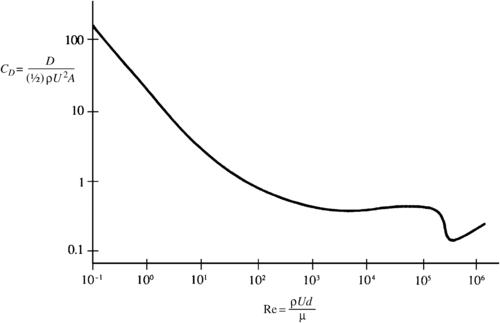
Figure 4.23 Coefficient of drag CD for a sphere vs. the Reynolds number Re based on sphere diameter. At low Reynolds number CD ∼ 1/Re, and above Re ∼ 103, CD ∼ constant (except for the dip between Re = 105 and 106). These behaviors (except for the dip) can be explained by simple dimensional reasoning. The reason for the dip is the transition of the laminar boundary layer to a turbulent one, as explained in Chapter 10.
Consider the flow of a fluid having nominal density ρ and viscosity μ through a flow field characterized by a length scale l, a velocity scale U, and a rotation or oscillation frequency Ω. The situation here is intended to be general so that the dimensional parameters obtained from this effort will be broadly applicable. Particular situations that would involve all five parameters include pulsating flow through a tube, flow past an undulating self-propelled body, or flow through a turbomachine.
The starting point is the Navier-Stokes momentum equation (4.39) simplified for incompressible flow. (The effect of compressibility is deduced from the continuity equation in the next subsection.)
 (4.39b)
This equation can be rendered dimensionless by defining dimensionless variables:
 (4.100)
where g is the acceleration of gravity. When these dimensionless variables are used, the boundary conditions can be stated in terms of pure numbers and are independent of l, U, and Ω. For example, consider the viscous flow over a circular cylinder of radius R. When the velocity scale U is the free-stream velocity and the length scale is the radius R, then, in terms of the dimensionless velocity u∗ = u/U and the dimensionless coordinate r∗ = r/R, the boundary condition at infinity is u∗ → 1 as r∗ → ∞, and the condition at the surface of the cylinder is u∗ = 0 at r∗ = 1. In addition, because pressure enters (4.39b) only as a gradient, the pressure itself is not of consequence; only pressure differences are important. The conventional practice is to render p − p∞ dimensionless, where p∞ is a suitably chosen reference pressure. Depending on the nature of the flow, p − p∞ could be made dimensionless with a generic viscous stress μU/l, a hydrostatic pressure ρgl, or as in (4.100), a dynamic pressure ρU2. Substitution of (4.100) into (4.39) produces:
 (4.101)
where ∇ ∗ = l ∇  . The form of this equation implies that two flows having different values of Ω, U, l, g, or μ, will obey the exactly the same differential momentum equation if the values of the dimensionless groups Ωl/U, gl/U2, and μ/ρUl are identical. Because the dimensionless boundary conditions are also identical in the two flows, it follows that they will have the same dimensionless solutions. Products of these dimensionless groups appear as coefficients in front of different terms when the pressure is presumed to have alternative scalings (see Exercise 4.71).
. The form of this equation implies that two flows having different values of Ω, U, l, g, or μ, will obey the exactly the same differential momentum equation if the values of the dimensionless groups Ωl/U, gl/U2, and μ/ρUl are identical. Because the dimensionless boundary conditions are also identical in the two flows, it follows that they will have the same dimensionless solutions. Products of these dimensionless groups appear as coefficients in front of different terms when the pressure is presumed to have alternative scalings (see Exercise 4.71).The parameter groupings shown in [,]-brackets in (4.100) have the following names and interpretations:
 (4.102)
 (4.103)
 (4.104)
The Strouhal number sets the importance of unsteady fluid acceleration in flows with oscillations. It is relevant when flow unsteadiness arises naturally or because of an imposed frequency. The Reynolds number is the most common dimensionless number in fluid mechanics. Low Re flows involve small sizes, low speeds, and high kinematic viscosity such as bacteria swimming through mucous. High Re flows involve large sizes, high speeds, and low kinematic viscosity such as an ocean liner steaming at full speed.
St, Re, and Fr have to be equal for dynamic similarity between two flows in which unsteadiness, and viscous and gravitational effects are important. Note that the mere presence of gravity does not make the gravitational effects dynamically important. For flow around an object in a homogeneous incompressible fluid, gravity is important only if surface waves are generated. Otherwise, the effect of gravity is simply to add a hydrostatic pressure to the entire system that changes the local pressure reference (see “Neglect of Gravity in Constant Density Flows” in Section 4.9).
Interestingly, in a density-stratified fluid, gravity can play a significant role without the presence of a free surface. The effective gravity force per unit volume in a two-fluid-layer situation is (ρ2 − ρ1)g, where ρ1 and ρ2 are fluid densities in the two layers. In such a case, an internal Froude number is defined as:
 (4.105)
where g′ ≡ g (ρ2 − ρ1)/ρ1 is the reduced gravity. For a continuously stratified fluid having a maximum buoyancy frequency N (see 1.35), the equivalent of (4.105) is Fr ′ ≡ U / N l  . Alternatively, the internal Froude number may be replaced by the Richardson Number =
 Ri ≡ 1 / Fr ′ 2 = g ′ l / U 2  , which can also be refined to a gradient Richardson number
 ≡ N 2 ( z ) / ( d U / d z ) 2  that is important in studies of instability and turbulence in stratified fluids.
. Alternatively, the internal Froude number may be replaced by the Richardson Number = , which can also be refined to a gradient Richardson number that is important in studies of instability and turbulence in stratified fluids.Under dynamic similarity, the dimensionless numbers in the model-scale flow are matched to their counterparts in the larger- or smaller-scale flow, and this ensures that the dimensionless solutions are identical. Furthermore, the dimensional consistency of the equations of motion ensures that all flow quantities may be set in dimensionless form. For example, the local pressure at point x = (x, y, z) can be made dimensionless in the form:
 (4.106)
where Cp = (p − p∞)/(½)ρU2 is called the pressure coefficient (or the Euler number = Eu), and Ψ represents the dimensionless solution for the pressure coefficient in terms of dimensionless parameters and variables. The factor of ½ in (4.106) is conventional but not necessary. Similar relations also hold for any other dimensionless flow variable such as velocity u/U. It follows that in dynamically similar flows, dimensionless flow variables are identical at corresponding points and times (that is, for identical values of x/l, and Ωt). Of course there are many instances where the flow geometry may require two or more length scales: l, l1, l2, … ln. When this is the case, the aspect ratios l1/l, l2/l, … ln/l provide a dimensionless description of the geometry, and would also appear as arguments of the function Ψ in a relationship like (4.106). Here a difference between relations (4.99) and (4.106) should be noted. Equation (4.99) is a relation between overall flow parameters, whereas (4.106) holds locally at a point.
Incidentally, in liquid flows, when p∞ in (4.106) is replaced by the liquid's vapor pressure, pυ, the dimensionless ratio is known as the cavitation number. Zero or negative cavitation number at any point in a flow indicates likely vapor-bubble formation at that location, and the presence of such bubbles may completely change the character of the flow, often in detrimental ways. For example, cavitation often sets performance limits and/or dictates the operational lifetime of hydrodynamic machinery such as water pumps, hydroelectric power turbines, and ship propellers.
In the foregoing analysis, the imposed unsteadiness in boundary conditions was assumed important. However, time may also be made dimensionless via t∗ = Ut/l, as would be appropriate for a flow with steady boundary conditions. In this case, the time derivative in (4.39) should still be retained because the resulting flow may still be naturally unsteady since flow oscillations can arise spontaneously even if the boundary conditions are steady. But, from dimensional considerations, such unsteadiness must have a time scale proportional to l/U.
In the foregoing analysis we have also assumed that an imposed velocity U is relevant. Consider now a situation in which the imposed boundary conditions are purely unsteady. To be specific, consider an object having a characteristic length scale l oscillating with a frequency Ω in a fluid at rest at infinity. This is a problem having an imposed length scale and an imposed time scale 1/Ω. In such a case a velocity scale U = lΩ can be constructed. The preceding analysis then goes through, leading to the conclusion that St = 1, Re = Ul/v = Ωl2/v, and Fr = U/(gl)1/2 = Ω(l/g)1/2 have to be duplicated for dynamic similarity.
All dimensionless quantities are identical in dynamically similar flows. For flow around an immersed body, like a sphere, we can define the (dimensionless) drag and lift coefficients:
 (4.107, 4.108)
where A is a reference area, and FD and FL are the drag and lift forces, respectively, experienced by the body; as in (4.106) the factor of ½ in (4.107) and (4.108) is conventional but not necessary. For blunt bodies such as spheres and cylinders, A is taken to be the maximum cross section perpendicular to the flow. Therefore, A = πd2/4 for a sphere of diameter d, and A = bd for a cylinder of diameter d and length b, with its axis perpendicular to the flow. For flows over flat plates, and airfoils, on the other hand, A is taken to be the planform area, that is, A = sl; here, l is the average length of the plate or chord of the airfoil in the direction of flow and s is the width perpendicular to the flow, sometimes called the span.
The values of the drag and lift coefficients are identical for dynamically similar flows. For flow about a steadily moving ship, the drag is caused both by gravitational and viscous effects so we must have a functional relation of the form CD = CD(Fr, Re). However, in many flows gravitational effects are unimportant. An example is flow around a body that is far from a free surface and does not generate gravity waves. In this case, Fr is irrelevant, so CD = CD(Re) is all that is needed when the effects of compressibility are unimportant. This is the situation portrayed by the first member of (4.99) and illustrated in Figure 4.23.
A recurring limitation in scale-model testing is the inability to match Reynolds numbers to achieve full dynamic similarity between a model and a larger and/or faster full-scale device. This situation is commonly known as incomplete similarity, and it can be managed in a variety of ways. First of all, if model- and full-scale Reynolds numbers cannot be matched with the same fluid, then use of a special fluid with a desirable density or viscosity for the model tests may be possible. Thus, hydrodynamic tests are sometimes performed on aerodynamic devices because the kinematic viscosity of water is approximately 1/15 that of air, so smaller devices tested at lower speeds in water can achieve the same Reynolds number as larger ones tested in faster moving air. Compressed air and liquid helium are other fluids that allow high-Reynolds number testing of model-scale devices. Second, the scale-model tests may show that the important performance metrics (CL and CD perhaps) are independent of Re above a threshold Reynolds number. In this case, model-to-full-scale extrapolation of performance results can be successful, but such extrapolation is inherently risky. However, such extrapolation uncertainty and risk from incomplete similarity in scale-model tests can be reduced if the model- and full-scale Reynolds numbers are as close as possible. In practice, this means that scale-model tests are typically conducted with the largest possible models at the highest possible speeds the available resources will allow. The two examples at the end of this subsection both describe performance predictions based on incomplete similarity.
Now return to the development of the dimensionless groups that naturally arise from the equations of motion. A dimensionless form of the continuity equation should indicate when flow-induced pressure differences induce significant departures from incompressible flow. However, the simplest possible scaling fails to provide any insights because the continuity equation itself does not contain the pressure. Thus, a more fruitful starting point for determining the relative size of ∇ · u  is (4.9):
is (4.9): (4.9)
(4.9)
along with the assumption that pressure-induced density changes will be isentropic, dp = c2dρ where c is the sound speed, see (1.25). Using the following dimensionless variables:
 (4.109)
 (4.110)
which specifically shows that the square of:
 (4.111)
sets the size of isentropic departures from incompressible flow. In engineering practice, gas flows are considered incompressible when M < 0.3, and from (4.110) this corresponds to ∼10% departure from ideal incompressible behavior when (1/ρ∗)(Dp∗/Dt∗) is unity. Of course, there may be nonisentropic changes in density too and these are considered in Thompson (1972, pp. 137–146). Flows in which M < 1 are called subsonic, whereas flows in which M > 1 are called supersonic. At high subsonic and supersonic speeds, matching Mach number between flows is required for dynamic similarity.
There are many possible thermal boundary conditions for the energy equation, so a fully general scaling of (4.60) is not possible. Instead, a simple scaling is provided based on constant specific heats, neglect of μυ, and constant free-stream and wall temperatures, To and Tw, respectively. In addition, for simplicity, an imposed flow oscillation frequency is not considered. The starting point of the scaling provided here is a mild revision of (4.60) that involves the enthalpy h per unit mass:
 (4.112)

 (4.113)
 (4.114)
Here the relevant dimensionless parameters are:
 (4.115)
 (4.116)
and we recognize ρ o U l / μ o  as the Reynolds number in (4.114) as well. In low speed flows, where the Eckert number is small the middle terms drop out of (4.109), and the full energy equation (4.107) reduces to (4.89). Thus, low Ec is needed for the Boussinesq approximation.
as the Reynolds number in (4.114) as well. In low speed flows, where the Eckert number is small the middle terms drop out of (4.109), and the full energy equation (4.107) reduces to (4.89). Thus, low Ec is needed for the Boussinesq approximation.The Prandtl number is a ratio of two molecular transport properties. It is therefore a fluid property and independent of flow geometry. For air at ordinary temperatures and pressures, Pr = 0.72, which is close to the value of 0.67 predicted from a simplified kinetic theory model assuming hard spheres and monatomic molecules (Hirschfelder, Curtiss, & Bird, 1954, pp. 9–16). For water at 20°C, Pr = 7.1. Dynamic similarity between flows involving thermal effects requires equality of the Eckert, Prandtl, and Reynolds numbers.
And finally, for flows involving surface tension σ, there are several relevant dimensionless numbers:
 (4.117)
 (4.118)
 (4.119)
Here, for the Weber and Bond numbers, the ratio is constructed based on a ratio of forces as in (4.107) and (4.108), and not forces per unit volume as in (4.103), (4.104), and (4.111). At high Weber number, droplets and bubbles are easily deformed by fluid acceleration or deceleration, for example during impact with a solid surface. At high Bond numbers surface tension effects are relatively unimportant compared to gravity, as is the case for long-wavelength, ocean surface waves. At high capillary numbers viscous forces dominate those from surface tension; this is commonly the case in machinery lubrication flows. However, for slow bubbly flow through porous media or narrow tubes (low Ca) the opposite is true.
Example 4.16
A ship 100 m long (l) is expected to cruise at 10 m/s (U). It has a submerged surface of 300 m2 (A). Find the model speed for a 1/25 scale model, neglecting frictional effects. The drag force FD is measured to be 60 N when the model is tested in a towing tank at this model speed. Estimate the full scale drag when the skin-friction drag coefficient for the model is 0.003 and that for the full-scale ship is 0.0015.
Solution
The ship's hull will interact with the water's surface and directly with the water, so both wave drag and friction drag will occur. In dimensionless form, this requires a dimensionless drag force to depend on the Froude number, the Reyonlds number, and an aspect ratio:
where Ψ is an undetermined function. Here it will not be possible to match both Fr and Re between the model and the full-scale device. However, the aspect ratio is matched automatically for a true scale-model test so it's not considered further.
To find the model test speed, equate the model and ship Froude numbers:

Here subscripts “m” and “s” denote model and ship parameters, respectively.
The total drag on the model is measured to be 60 N at this model speed, and part of this is friction drag. Here we can use Froude's hypothesis that the unknown function Ψ is a sum of a frictional drag term Ψf that only depends on the Reynolds number (and surface roughness ratio), and a wave drag term Ψw that only depends on the Froude number.
Futhermore, treat the submerged portion of the hull as a flat plate for which the friction drag coefficient CD is a function of the Reynolds number, i.e., set CD = Ψf. The problem statement sets the frictional drag coefficients as CD,m = 0.003 and CD,s = 0.0015, and these are consistent with the length-based Re values for the model and the ship, 8 × 10 6  and 109, respectively. Using a value of ρ = 1000 kg/m3 for water, the model’s friction drag can be estimated:
and 109, respectively. Using a value of ρ = 1000 kg/m3 for water, the model’s friction drag can be estimated:
Thus, out of the total model drag of 60 N, the model's wave drag is (FWD)m = 60 − 2.88 = 57.12 N. And this wave drag obeys the scaling law above, which means that:

Thus, the wave drag on the ship (FWD)s can be estimated as follows:

where the area ratio is the square of the length-scale ratio. To this must be added the ship’s frictional drag:

Therefore, total drag on ship is predicted to be: (8.925 + 0.225) × 105 = 9.15 × 10⁵ N. If no correction was made for friction, and all the measured model drag was assumed due to wave effects, then the prediced ship drag would be:

which is a few percent higher than the friction-corrected estimate.
Example 4.17
A table top centrifugal blower with diameter of d1 is tested at rotational speed Ω1 and generates a volume flow rate of Q1 against a pressure difference of Δp1 when moving air with density ρ1 and viscosity μ1. What are the three relevant dimensionless groups? A scale-similar centrifugal water pump with diameter d2 = 2d1 is operated at rotational speed Ω2 = Ω1/10. If turbomachine performance is independent of Re in the operational range of these devices, what are the pump’s volume flow rate Q2 and pressure rise Δp1 if Re is not matched but the other two dimensionless parameters are?
Solution
Dimensional analysis using the six parameters yields the following dimensionless groups:

These three, along with the device's efficency, are routinely used when scaling turbomachine performance. Matching flow coefficients produces:
Matching head coefficients produces:

where the water/air-density ratio is 825 at room temperature and pressure. For these conditions, the water pump power is Q2Δp2 = 26.4Q1Δp1, a substantial increase above the blower's power. And, the Reynolds number ratio is:
where ν is the kinematic viscosity and ν2/ν1 ≈ 1/15 at room temperature and pressure.