15.2. Acoustics

Perhaps the simplest and most common form of compressible flow is found when the variations in velocity, pressure, and density are small compared to steady reference values and the variations in pressure and density are isentropic. This branch of compressible flow is known as acoustics and is concerned with the study of sound waves. Acoustics is the small disturbance theory of compressible fluid dynamics and is a broad field with its own rich history (see Pierce, 1989). The primary concern in this section is to show how the speed of sound enters the equations for compressible flow, to deduce how pressure disturbances may arise in such flows, and to develop some insight into the behavior of pressure disturbances in compressible flow by considering solutions of the linearized equations of motion.

The development starts from the mass and momentum conservation equations for a moving single-component viscous fluid [see (4.8) and (4.38)] modified to include source terms:

1ρDρDt+∂ui∂xi=q,andDujDt+1ρ∂p∂xj=gj+1ρ∂τij∂xi+fj,

(15.4, 15.5)

where τ_ij is the viscous stress tensor given by (4.36). The added source term in (15.4), q(x_i,t), is an unsteady volume source distribution (per unit volume), and the added source term in (15.5), f_j(x_i,t), is an unsteady body-force distribution (per unit mass of fluid). Both represent acoustic sources not produced directly by fluid motion. These terms may be non-zero because of naturally occurring or anthropogenic acoustic sources (voices, animal calls, loud speakers, transducers, unsteady combustion, unsteady heat transfer, vibrating structures, rotating fan or propeller blades, etc.). Alternatively, these source terms can often be specified through initial and boundary conditions; however, their placement in (15.4) and (15.5) is common in acoustic analysis.

Acoustic waves in fluids are lightly-damped small-amplitude isentropic pressure fluctuations so pressure and density fluctuations are assumed to be isentropic following a fluid particle. Thus, τ_ij in (15.5) is commonly ignored unless the acoustic frequency is very high or the propagation distance is very long. The equation associated with the isentropic assumption can be obtained by D/Dt-differentiating the equation of state for the pressure p = p(ρ,s), setting Ds/Dt = 0, and using (1.25) for c²:

DpDt=(∂p∂ρ)sDρDt+(∂p∂s)ρDsDt=c2DρDt.

(15.6)

The variations in p and ρ accommodated by (15.6) include acoustic waves, and other isentropic density and pressure variations. Non-isentropic fluctuations, such as strong shock waves and compressible turbulence, are omitted. However, the acoustic effects of many non-isentropic processes such as thermal conduction, viscous dissipation, radiative energy transfer, chemical reactions, and phase change can be reintroduced to this formulation via the q and f_j source terms in (15.4) and (15.5).

A general wave equation for the pressure p can be assembled from (15.4), (15.5), and (15.6) by substitution and cross differentiation (see Exercise 15.1):

DDt(1ρc2DpDt)−∂∂xj(1ρ∂p∂xj)=DqDt−∂fj∂xj+∂ui∂xj∂uj∂xi,

(15.7)

where τ_ij has been dropped to be consistent with (15.6), and the steady body force (gravity) has been presumed spatially uniform so that ∂g_j/∂x_j = 0. Although (15.7) incorporates several dependent variables (p, ρ, u_i), it serves to identify the acoustic source terms. This left side of (15.7) is a convected wave operator modified to account for varying fluid velocity, varying fluid density, and varying sound speed. The right side of (15.7) displays three source terms corresponding to unsteady expansion within the fluid domain (monopole sources), the divergence of spatially-varying fluctuating body forces (dipole sources), and the interaction of the moving fluid with itself (quadrupole sources), respectively. For convenience, these may be combined:

q˙≡DqDt−∂fj∂xj+∂ui∂xj∂uj∂xi,

(15.8)

since all three are scalars and since dipoles and quadrupoles can be constructed from weighted super positions of monopoles. Here it should be noted that the aero-acoustic equivalent of (15.7) is typically formulated differently (see Lighthill, 1952 or Crighton, 1975).

To reduce (15.7) to a solvable equation for acoustic pressure fluctuations, several additional simplifications beyond that inherent in (15.6) are commonly made. First, the various dependent field variables are separated into nominally steady and fluctuating acoustic values:

ui=Ui+ui′,p=p0+p′,ρ=ρ0+ρ′,andT=T0+T′,

(15.9)

where U_i, p₀, ρ_0, and T₀ are constants applicable to the region of interest, and all the fluctuating quantities – denoted by primes in (15.9) – are considered to be small compared to these. In addition, if the flow is isentropic in the realm of interest, the pressure can to be Taylor expanded about the reference thermodynamic state specified by p₀ and ρ₀:

p=p0+p′=p0+(∂p∂ρ)s(ρ−ρ0)+12(∂2p∂ρ2)s(ρ−ρ0)2+…=p0+c2ρ′+12(∂2p∂ρ2)sρ′2+…

For small isentropic variations, the second-order and higher terms can be neglected, and this leads to a simple relationship between acoustic pressure and density fluctuations that replaces (15.6):

p′=c2ρ′.

(15.10)

This equation is valid when the fractional density change or condensation = ρ′/ρ₀ = p′/ρ₀c² is small:

p′/ρ0c2≪1.

(15.11)

For ordinary sound levels in air, acoustic-pressure magnitudes are of order 1 Pa or less, so the ratio specified in (15.11) is typically less than 10^–5 since ρ₀c² = γp₀ ≈ 1.4 × 10⁵ Pa. Additionally, positive p′ is called compression while negative p′ is called expansion (or rarefaction). Acoustic pressure disturbances are commonly composed of equal amounts of compression and expansion.

The first approximate expression for c was found by Newton, who assumed that p′/p₀ was equal to ρ′/ρ₀ (Boyle's law) as would be true if the process undergone by a fluid particle was isothermal. In this manner Newton arrived at the expression c = [RT]^1/2. He attributed the discrepancy of this formula with experimental measurements as due to “unclean air.” However, the science of thermodynamics was virtually non-existent at the time, so that the idea of an isentropic process was unknown to Newton. The correct expression for the sound speed was first given by Laplace.

The usual field equation for acoustic pressure disturbances can be obtained from (15.7) without source terms by inserting (15.9) and linearizing with U_i, p₀, ρ₀ and T₀ treated as time-invariant and spatially uniform. The resulting equation is the field equation for acoustic pressure disturbances in a uniform flow:

1c2(∂∂t+Ui∂∂xi)2p′−∂2p′∂xi∂xi=0,

(15.12)

(see Exercise 15.2).

To highlight the importance of the sound speed, consider a stationary fluid and one-dimensional pressure disturbances. For a stationary fluid (U_i = 0), (15.12) reduces to:

1c2∂2p′∂t2−∂2p′∂xi∂xi=0,

(15.13)

and this is the classical wave equation for acoustic waves in a lossless uniform medium. Under these same circumstances, the simplified and linearized version of (15.5) provides the relationship between acoustic pressure and fluid velocity fluctuations:

∂uj′∂t+1ρ0∂p′∂xj=0oruj′(x,t)=−1ρo∫∂p′∂xjdt.

(15.14)

When the pressure disturbances are one-dimensional and only vary along the x₁-axis, then (15.13) reduces to the one-dimensional wave equation and its solutions are of the form:

p′(x,t)=f(x−ct)+g(x+ct),

(15.15)

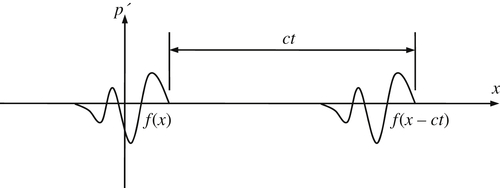
where x₁ = x, and the functions f and g are determined by initial conditions (see Exercise 15.3). Equation (15.15) is known as d'Alembert's solution, and f(x – ct) and g(x + ct) represent traveling pressure disturbances that propagate to the right and left, respectively, with increasing time. Consider a pressure pulse p′(x,t) that propagates to the right and is centered at x = 0 with shape f(x) at t = 0 as shown in Figure 15.1. An arbitrary time t later, the wave is centered at x = ct and its shape is described by f(x – ct). Similarly, when p′(x,t) = g(x + ct), the pressure disturbance propagates to the left and is located at x = –ct at time t. Thus, the speed at which acoustic pressure disturbances travel is c, and this is independent of the shape of the pressure disturbance waveform.

However, the disturbance waveform does influence the fluid velocity, u′, along the x-axis. It can be determined from (15.14) and (15.15) with x₁ = x, and is given by:

u1′(x,t)=1ρ0c(f(x−ct)−g(x+ct))

(15.16)

(see Exercise 15.4). Thus, the fluid velocity includes rightward- and leftward-propagating components that are matched to the pressure disturbance. Moreover, (15.16) shows that the compression portions of f and g lead to fluid velocity in the same direction as wave propagation; the fluid velocity from f(x – ct) is to the right when f > 0, and the fluid velocity from g(x + ct) is to the left when g > 0. Similarly, the expansion portions of f and g lead to fluid velocity in the direction opposite of wave propagation; the fluid velocity from f(x – ct) is to the left when f < 0, and the fluid velocity from g(x + ct) is to the right when g < 0. These fluid velocity directions are worth noting because they persist with the same signs when the wave amplitudes exceed those allowed by the approximation (15.11).

Now consider one-dimensional pressure waves p′(x,t) when U_i = (U, 0, 0) so that (15.12) becomes:

1c2(∂∂t+U∂∂x)2p′−∂2p′∂x2=0.

The general solution of this equation is:

p′(x,t)=f(x−(c+U)t)+g(x+(c−U)t).

(15.17)

Figure 15.1 Propagation of an acoustic pressure disturbance p′ that travels to the right with increasing time. At t = 0 the disturbance is centered at x = 0 and has waveform f(x). At time t later, the disturbance has moved a distance ct but its waveform shape has not changed.

When U > 0, the travel speed of the downstream-propagating waves is enhanced and that of the upstream-propagating waves is reduced. However, when the flow is supersonic, U > c, both portions of (15.17) travel downstream, and this represents a major change in the character of the flow. In subsonic flow, both upstream and downstream pressure disturbances may influence the flow at the location of interest, while in supersonic flow only upstream disturbances may influence the flow. For aircraft moving through a nominally quiescent atmosphere, this means that a ground-based observer below the aircraft's flight path may hear a subsonic aircraft before it is overhead. However, a supersonic aircraft does not radiate sound forward in the direction of flight so the same ground-based observer will only hear a supersonic aircraft after it has passed overhead (see Section 15.9).

Linear acoustic theory is valuable and effective for weak pressure disturbances, and it also indicates how nonlinear phenomena arise as pressure-disturbance amplitudes increase. The speed of sound in gases depends on the local temperature, c = [γRT]^1/2. For air at 15°C, this gives c = 340 m/s. The nonlinear terms that were dropped in the linearization leading to (15.12) may change the waveform of a propagating nonlinear pressure disturbance depending on whether it is a compression or expansion. Because γ > 1, the isentropic relations show that if p′ > 0 (compression), then T′ > 0 so the sound speed c increases within a compression disturbance. Therefore, pressure variations within a region of nonlinear compression travel faster than a zero-crossing of p′ where c = [γRT₀]^1/2 and therefore may catch up with the leading edge of the compressed region. Such compression-induced changes in c cause nonlinear compression waves to spontaneously steepen as they travel. The opposite is true for nonlinear expansion waves where p′ < 0 and T′ < 0, so c decreases. Here, any pressure variations within the region of expansion fall farther behind the leading edge of the expansion. This causes nonlinear expansion waves to spontaneously spread or flatten as they travel. When combined these effects cause a nonlinear sinusoidal pressure disturbance involving equal amounts of compression and expansion to evolve into a saw-tooth shape (see Chapter 11 in Pierce, 1989). Pressure disturbances that do not satisfy the approximation (15.11) are called finite amplitude waves.

The limiting form of a finite-amplitude compression wave is a discontinuous change of pressure, commonly known as a shock wave. In Section 15.6 it will be shown that the finite-amplitude compression waves are not isentropic and that they propagate through a still fluid faster than acoustic waves.

Example 15.2

For airborne sound, the decibel scale is defined by: SPL = 20log₁₀[p_rms/p_ref], where SPL is sound pressure level in dB (the abbreviation for decibels), p_rms is the root-mean-square pressure amplitude of the sound of interest, and p_ref = 20 μPa (an international standard). Here, p_ref is chosen so that 0 dB corresponds to quiet sounds at the nominal threshold of human hearing. Using this information, assess the validity of (15.11) for sounds with SPL = 30 dB (soft whispering), 60 dB (normal conversation), 90 dB (noisy factory), 115 dB (good seat at a rock concert), 130 dB (near an aircraft engine), and 160 dB (inside of an automobile exhaust system) at atmospheric pressure.

Solution

The definition of SPL can be inverted to find p_rms = p_ref10^(SPL/20), and ρ₀c² = γp₀ ≈ 140 kPa at atmospheric pressure. Thus, for SPL = 30 dB, (15.11) becomes:

prms/ρ0c2=(20μPa)10(30/20)/(140kPa)=4.5×10−9≪1,

 

and the small amplitude requirement for linear acoustics is well satisfied. The remaining SPL values lead to the following numbers:

60dB:prms/ρ0c2=1.4×10−7,90dB:prms/ρ0c2=4.5×10−6,115dB:prms/ρ0c2=8.0×10−5,130dB:prms/ρ0c2=4.5×10−4,160dB:prms/ρ0c2=1.4×10−2.

 

Thus, even at decibel levels that cause hearing damage (130 dB) or deafness (160 dB), the small-amplitude requirement for linear acoustics is met. Therefore, the linear theory of acoustics applies throughout (and somewhat beyond) the amplitude range of human hearing.