1.1 Basics of Networked Control Systems
A Networked Control System (NCS) is a particular kind of a real-time distributed system (RTDS), composed of a set of nodes, interconnected by a network, able to develop a control process. A NCS is a dynamic control system where the control loops are closed through a communication network. The main feature of a NCS is that the control signal, the feedback signal or both are exchanged among the system’s components in a network, interchange information packages through a network.
Main components of a control process are sensors, controllers and actuators, which rely on a real-time operating system and a communication network. NCSs have received increasing attention in the last few years, due to several advantages, such as an easy maintenance, a high reliability, less wiring, and low cost. Besides, the use of control network architectures, when properly applied, may improve efficiency, flexibility, and reliability, reducing installation, reconfiguration, maintenance in time, and costs.
Nevertheless, notice that the use of a single communication network for all control signals (e.g. control and feedback) modify the performance of the whole NCS. This is due because the network generates some imperfections in packet transmission, such as time delays, packet loss, etc. Furthermore, conventional standard results in analysis and design of digital control theory cannot be used, since many of its assumptions are not directly applicable to NCS, specifically considering time delays and packet loss. The use of common bus network topology introduces different forms of uncertainties between sensors, actuators, and controllers. Several approaches have been developed to tackle this problem, mainly based on the work of Halevi and Ray [1]. In such approaches, a group of nodes make use of the same network, producing a traffic load. If there is no coordination among the nodes, some nodes may transmit simultaneously, this generates time-delays, retransmissions, or worst, packet loss. This results in packets which are unable to fulfil their deadlines. In order to achieve overall objectives of all message send in a NCS, it is necessary for all nodes to properly exchange their own information through the network. Therefore, the mechanism to exchange information plays an important role in the stability and performance of the NCS implemented over a communication network.
In a NCS, the main problems that degrade its performance are network-induced delays and packet loss. Time delays can be constant, time-varying or even random; those depend on the scheduler, network type, architecture, operating systems, etc. [2]. When a NCS uses a reliable network, it is possible to compensate for time delays, lower or larger than the sampling period obtaining their bounds. However, when a NCS uses an unreliable network, it is more difficult to compensate for unknown time delays and packet loss, and these reduce the efficiency of NCS.
NCSs have been studied for the last 20 years, using several assumptions regarding time delays modelling, or uncertainties accomplishment. In this book, some network imperfections are modelled, in order to be coupled with a control law design. Several strategies are reviewed, such as fuzzy approximation, frequency communication modelling, or dynamic scheduling procedure. All of them trigger certain threshold onto dynamic systems models. However, the modelling procedure for NCSs is a challenge, since there are several non-linear situations, like saturation, unknown time delays, dead-zones, etc., with which it is necessary to deal. Other static strategies, like digital control, are unable to produce a feasible result since time delays are variable.
As previously stated, time delays are dynamic as a result of computer network interaction. Therefore, to study such behaviour provides a good approximation of how time delays behave in several situations, like overflowing, fault appearance, packet loss, or undersampling time delays.
NCS, since its beginning, employed classic control techniques such as linear control, adaptable control, robust control, and so on, with some modifications to compensate the imperfections due to the network [3]. Such techniques, as it is common in classic control theory, are divided into techniques in the continuous dominion [4] and techniques in the discrete domain [5–7]. Fridman and Shaked [8] introduced a model transformation for the delay-dependent stability of systems with time-varying delays in terms of LMIs. Their model also refined results from delay-dependent H control and extended them to the case of time-varying delays.
Although the field of NCS is still relatively new, many research approaches have been developed in it. Most of them work on a single imperfection due to the network. Results present in the literature should be extended and integrated to simultaneously obtain a reference framework and study imperfections due to the network. Here, a revision of the literature around NCS is presented, focusing on methods that compensate several imperfections, and distinguishing design methodologies. Some of the techniques only compensate a single imperfection, such as time delays or packet loss as the most common ones, since both of them highly degrade the system performance. Later, some methods that tackle the combination of several imperfections are introduced, setting their advantages and liabilities.
The later techniques to design NCSs leave aside concepts established by communication networks, by supposing some features due to the network, like for example the maximum delay, its derivative, or the packet loss, as well as the assumption about the execution of strictly periodic nodes, and the synchronisation among them. Almost every imperfection arising from the process itself as plant delays [9].
In the last few years, the concept of co-design has been used to name the application of multiple knowledge areas together, aiming for solving a common problem. The most common co-design technique for NCS is based on control-communication, whose objective is to design a NCS through a controller observing network features, and a scheduler considering control aspects for the transmission between nodes.
As part of a co-design approach, it is especially important to take into consideration the multiple imperfections due to the network, not only for the controller design but also for the scheduler. For example, reducing the quantization error (by transmitting packets with more bits) normally results in longer time delays that have to be compensated, in the network by the scheduler, or in the process through a controller. Performing co-design assumes compensating the NCS as a whole (process, controller, scheduler), in an integral way, which makes necessary the use of tools to obtain quantitative information from the control system and the network.
1.2 Sources of Uncertainties
- 1.
Quantization error
- 2.
Packet loss
- 3.
Variant sampling interval/period
- 4.
Communication delays
- 5.
Communication limitations.
The presence of any of these uncertainties may degrade the performance of the system, even reaching instability. Based on this, it is important then to understand how these phenomena influence the stability of the system and its performance. Unfortunately, most of the available literature focuses only on a subset of them, while ignoring the rest. For example, systematic methods analyse the stability of NCSs considering only some imperfection. Quantization errors, for instance, are studied in [10–16].
In practice, almost all uncertainties of the network are present in a NCS. This makes necessary methods for analysis and synthesis that include most, if not all of these uncertainties, to compensate them. Very few results have been reported that integrate compensation for multiple uncertainties.
Modelling the network imperfections or modelling the network behaviour with imperfections, in several cases, is a prerequisite for control design, these models depend on the kind of network, the used protocol, and so on. The most common classification of time delays is proposed by Nilsson [2]. Three different models are discussed: constant time delay, random time delay dependent on previous transmissions, and random time delay with probability distribution dependent on Markov chains.
However, the models of independent random time delay do not capture the effect of strong package traffic in the network (also refer to consumed bandwidth), which sometimes follows correlations between random time delays, where a time delay value depends on previous time delays. If the network experiences strong traffic, it is very probable that all packets suffer long transmission time delays, until the network load diminishes. If the network load considerably varies, a solution is to model it using time delay distributions by a Markov chain [2].
For modelling a time delay in a network with strong and variant traffic, the model of the network may need to have a state unless the variation is unbounded. The effect of variant traffic could be modelled using a Markov chain, which performs a transition each time there is a transference on the communication network, and thus, proposing probability distributions for the time delays between sensor-controller ( ), and controller-actuator (
 ) at each state.
One common strategy is the queue methodology, which uses observers and predictors to compensate the time delays, and ensures invariance through time of the NCS. Using the queue theory forces the random time delays to present a deterministic (constant) behaviour. The method presented by Luck and Ray [17] uses an observer to estimate the states of the plant, and a predictor to compute the predictive control based on measurements of past outputs. The control and the measurements of past outputs are stored as FIFO (First Input—First Output) queues in buffers. These are placed before and after the controller within the control loop. First, the past measurements are used for estimating the states of the plant in  , where k is the size of the buffer between sensor and observer. Then, using other estimations, the state of the plant is predicted at
  , where l is the size of the buffer after the controller. The predictive control signal
  is obtained and stored in the buffer. The observer and predictor are based on the dynamic model, and thus, the performance of the system is highly dependent on the precision of the model.
1.3 Communication Methodologies
Communication methodologies make use of computer science to design the network for the NCS and generating scheduling algorithms for the nodes and the network, aiming for maintaining the stability of the NCS. There are two main approaches: One characterises and designs the communication network [18–21]; and another design scheduling algorithms for the packet transmission through the network [22–25]. An objective of this approach is to keep the structure of the NCS, by establishing an Ethernet network without modification, and focussing on the scheduling methods.
Regarding scheduling, the pioneering work of Hong [22] proposes a scheduling algorithm to determine the sampling times by using the concept of a transmission window. Sampled data from the NCS components share a limited number of windows, so the performance requirements of each control loop are satisfied, but the utilisation of the network resources considerably increase. This methodology establishes time delays within a boundary, and avoiding packet collisions, applying to Polling and Token Passing systems.
Later, Pegden et al. [23] present an algorithm to assign bandwidth, applicable to the CAN protocol for NCS, using CSMA/NBA (Carrier Sense Multiple Access with Non-destructive Bitwise Arbitration) [26]. Each node watches the state of the bus before data transmission. Nodes delay data transmission until the bus is free. When the bus is free, any node may start transmission. If more than one node starts transmission at the same time, the bus enters in conflict, which requires solving a comparison of their identifiers. The algorithm to assign bandwidth satisfies the time delay requirements for real-time control and data for events, maximising the use of network bandwidth, and it is designed offline. It also presents the liability of being incapable of dynamically modify the assignment of data transmission, while the control system executes. Another liability is that it only takes into consideration time delays smaller than the sampling period.
Scheduling methodology provides that control actions are carried through events and no time, using the dynamics of the plant as triggers. Tarn and Xi et al. [27] propose a methodology based on events that use the movement of the system as a reference, instead of deciding the next sampling-action instant through time [28]. Such the action is started by an event, triggered by the system state or error. The method maps the time-space in the event-space, and thus, the stability of the system does not depend on time but the state’s position or the measured error. Hence, the induced delays by the network are smaller than the response times of the process, and they do not destabilise the system, nevertheless they maybe accumulative. However, if the delays are too large or there is packet loss, the performance of the system degrades.
Queue methodology makes use of observers and predictors for compensating delays, guaranteeing time invariance of the NCS through time. The methodology uses queue theory to force that random delays present a deterministic and constant behaviour. The method by Luck and Ray [17] uses an observer to estimate the states of the plant, and a predictor to obtain the predictive control, based on previous output measurements. The control and previous output measurements are stored as FIFO queues in buffers. These are placed before and after the controller in the closed loop. First, previous output measurements are used to estimate the states of the plant, where it is the register size between sensor and observer. Next, using previous estimations, the state of the plant is predicted. The predictive control signal is obtained and stored in the register, the observer and predictor are based on a model, and thus, the performance of the system is highly dependent on how precise is the model. Chan and Ozguner et al. [29] used to jump systems to design a static controller for a time-invariant system with a FIFO queue and the known maximum buffer size and the upper bound of random delay in the communication link. More recently, Filipovic [30] used to finite dimensional discrete-time jump linear systems with finite state Markov chains but a non-linear model of a queue in the sensor, the feedback linearization is used to linearize the queue. It means that in the control loop there are two controllers. The first one performs feedback linearization of the buffer and the second one is the main feedback controller.
Wang and Liu’s book [31] presents a review of the NCS systems in the past decade. It also presents a review of several scheduling protocols using in NCS like try-one-discard (TOD), Round-Robin (RR) persistently exciting (PE) constant penalty TOD (CP-TOD) etc., its advantages and disadvantages, finally presents an extensive stability analysis, other recient reviews are presented in [32].
1.4 Control Methodologies
The area of communications attempts to minimise, compensate, or eliminate the delays induced by the network, by an ordered assignment of transmission and maximising the resource utilisation. In the area of control, the intention is to incorporate the imperfections in the network model, and modifying the control techniques established for digital control and continuous control. The methods comprise optimal control, robust control, adaptive control, fuzzy control, stochastic control, and so on.
A common method is based on obtaining an augmented model in discrete time, which incorporates time delays in the network as a state of the system [1]. Also, time delays are considered as stochastic, and the objective is to design an optimal control [2]. Another recurrent approach is to suppose the delay as a perturbation of the system and compensate using control techniques to deal with perturbations [33]. The same happens using robust control for designing control laws that are not very sensitive to delays [36]. Adapting the control signal regarding the effect on the network is a method employed by fuzzy control and adaptable control, by modifying the controller gains.
For a review of other control methodologies can refer to Wang and Lius book [31] and introductions from [34, 35]. It presents diverse strategies such as predictive, h , fuzzy, multi-agent, Smith predictor and robust polynomial. The fuzzy control systems presented are developed in the continuous and discrete domain, one showed a h
 control for TSK (Takagi-Sugeno-Kang) systems with time delays, assuming synchronization of the nodes and only sensor-controller communication. The second uses a TSK model that considers the time delays and dropouts, modelling the imperfections as stochastic events. Both present simulation examples to prove their effectiveness. Also, Bemporad et al. book [37] presents a good review of the design characteristics for distributed control methodologies, from the selection and configuration of the network to the generation of middleware to minimize time and effort in the application. Performs a review of the modelling of wireless networks and its various topologies for NCS, An NCS review based on events is presented for its application in control, estimation and optimization.
The description of relevant methods and their evolution are described in the following paragraphs.
Halevi and Ray [1] propose an augmented method, augmenting the state space in the discrete-time model. Network delays are handled by the controller, using previously applied control signals as internal states for calculating a new control signal at the kth time. This generates a new model with the original states of the system and the previous inputs as new states. The stability for periodic delays is proven based on the eigenvalues of the transition matrix obtained of the augmented system.
Nilsson [2] develops an optimal control method for NCS. The delay is assumed as random, but smaller than the sampling period. Later Lincoln [38] extends the method for delays larger than the sampling period. The basic idea is to present the problem as a LQG (Linear Quadratic Gaussian) system. Dynamic systems are given in the space state, and the gain of the optimal controller is solved as a LQG problem, using dynamic programming. Solving this problem requires past delay information and the complete states.
The perturbation method, proposed by Walsh et al. [33], takes into consideration the difference between the actual output and the most recent transmitted output values as a perturbation of the system, searching the error boundaries. Stability is obtained using the Lyapunov method on the error dynamics. Several assumptions are established, including error-free communications, fast sampling, and noiseless observations. However, the process and controller may be non-linear and time variant. In this method, the network only sends from sensor to controller, and there is no exchange between controller and actuator. In [39], the networked control system is supposed for singularly perturbed systems with time-varying transmission times. The slow and fast systems of singularly perturbed systems are used to approximate the state behaviour. Under the condition that their systems are Hurwitz stable, the whole systems via the network control are robust practically stable if the perturbation parameter is sufficiently small.
In the robust control method, proposed by Goktas et al. [36], delays induced by the network are managed as perturbations of the nominal system. The controller design is carried out in the frequency domain, using robust control theory. The major advantage of this method is that it is not necessary to know beforehand the precision of the delay distribution. Network delays are supposed bounded, and they are modelled as simultaneous multiplicative perturbations. Thus, the  design synthesis can be applied, choosing certain multiplicative weights for uncertainties, such that the NCS would be not very sensitive to known delays.
The fuzzy control method takes advantage of fuzzy theory to update the gains of the controller based on the error signal between the reference and the actual output of the system and the controller output [40]. Actually, the method updates the gain of a PI (Proportional-Integral) controller based on the error and the controller output. The design includes member functions online and offline for optimisation. Zhang and Li et al. [41] obtain a delay for maximising the cross-correlation function of the output of the plant, estimated without delay, and the measured output. This estimation scheme uses a fuzzy Smith predictor that compensates the constant delay, and the fuzzy controller is used for adapting the changing parameters of the system.
The adaptive control is used for the modification of the system parameters provided counteract its dynamic changes. Thus optimising the control signals to each system behaviour. The adaptive control method for NCS is based on the ability to measure the traffic conditions of the network, adapting the controller parameters. In this method, the controller is able to sense and update the conditions of the Quality of Service (QoS) in the network. If the QoS requirements are not satisfied, the parameters of the controller are tuned, aiming to improve the performance as possible [42].
Packet loss is another network imperfection to highly take into consideration. In general literature, packet loss is modelled using two processes: a random Bernoulli process, or a typical Markov chain process. The results of the approaches that apply random Bernoulli assume that lost packets are independent and identically distributed (i.i.d.) [33, 43], while the other approaches that use Markov chains suppose that lost packets are streams, and occur in accordance with a Markov chain [44–46]. Most of the existing results design filters within the NCS to estimate the states of the system, with the feature of establishing an input zero, this is, when measurements are lost. With this configuration, the estimation with packet loss is called estimation with intermittent observations or loses [33, 43, 45, 46].
To estimate the system states with intermittent observations and to know the system behaviour with packet loss, to adapt a Kalman filter for the estimation is one of the most popular and useful methods for filtering problems. It has the disadvantages of supposing the knowledge of a precise model of the system and that the statistical information of external noise is already known. In [43], it is proposed the design of a Kalman filter using both packet loss models, Bernoulli i.i.d. and Gilbert-Elliot model (developed with discrete Markov chains with two states). Another result that employs a Kalman filter to estimate the states for linear, stochastic systems [33] takes into consideration the Bernoulli approach to model packet loss, as well as taking into consideration system uncertainties. Smith Y Seiler [45] employ a Kalman filter variant in simple time to estimate the states of the system, considering a Markov chains model for the lost packets. In [46] it is employed a discrete Kalman filter for packet modelling, using a binary probability distribution. The analysis and design of the filter provide a boundary in the arrival rate of measurements.
Another methodology for estimation is using filters, that provide a guarantee of noise attenuation and robustness over uncertainties of the model [47]. The filters for NCS have recently appeared [23, 47–49]. In [23], the filter is designed for a class of stochastic NCS with consecutive packet loss, separating the loss rate for sensor-controller communication and controller-actuator communication.
Regarding optimal controllers, Gupta et al. [50] developed a LQG controller for a link with a single packet lost between sensor and controller. It is assumed a linear process in discrete time, and without network induced delays within the control loop. The controller does not require information of the statistical model of the packet loss event. Imer et al. [51] and Sinopoli et al. [7] develop a LQG controller over unreliable communication links, comparing the performance of protocols such as TCP (Transmission Control Protocol) and UDP (User Datagram Protocol). Both studies model packet loss between sensor-controller link and controller-actuator link as Bernoulli i.i.d (Independent and Identically Distributed).
1.5 Co-Design Methodologies
Codesign has the objective of mixing the advantages of two or more knowledge areas and minimise the liabilities of such areas when presented separately, aiming to adequately resolve a common problem. In NCS, control-communication codesign commonly integrates feedback control and real-time communications. It is based on the principle that system performance depends on the design of control algorithms, and also relies on the scheduling performance of the shared communication resources. Unfortunately, NCS design is very frequently based on the principle of separation of concerns [52]. This principle assumes that feedback controllers can be modelled and implemented as periodic tasks with a fixed period, and known consumption (i.e. Worst Case Execution Time or WCET), and a rigid deadline. These assumptions are amply adopted by the control community and developed by sampling systems theory. Even though these assumptions allow the control community to focus on its own problems, without concerning about how scheduling is performed in the nodes and how packet in the network are carried out, as well as the communication community is not worried about understanding how scheduling impacts on system performance.
The control task does not always make use of the available computing resources in an optimal way, and the assumptions of the model of simple tasks are too restrictive regarding the characteristics of many control systems. For instance, many deadlines are not always rigid, that is, many practical control systems may occasionally tolerate losing a deadline.
To confront resource limitation in a NCS, co-design is necessary at different levels, for example, hardware/software codesign, or mechanic/electric codesign. Here, co-design is used at the control/communication level. This methodology can be divided into two categories: feedback control of computational systems and real-time control.
The category of feedback control of computational systems is also known as feedback scheduling [52]. The basic idea is dealing with the scheduling problem as a feedback control problem. A feedback control loop is introduced within the resource manager of the computer systems. The objective of feedback scheduling is increasing flexibility regarding the uncertainties in resource utilisation. Instead of pre-assigning resources based on an offline analysis, resources are online, dynamically assigned, based on the feedback from the utilisation of the actual resource and the execution times of control tasks.
Xia et al. [53] design a fuzzy feedback scheduling. Using a control loop and an outer feedback loop to implement the scheduling. The scheduler is to dynamically regulate the sampling periods to achieve a desired level of utilisation. The timing attributes of all non-control tasks cannot be changed by the feedback scheduler. Another work in this field is the fuzzy feedback scheduling based on output jitter, which is formulated in [54]. The output jitter is the controlled variable, and the CPU utilisation and jitter are the control inputs. So, when the system resource changes, the result is that some key periodic tasks still meet an expected jitter range regulating only the task periods.
The second category of codesign here focuses on real-time control. Branisky et al. [55] were among the first to establish that scheduling and control systems cannot be separately designed. They work on regulation problems of the plant as an optimal scheduling problem, observing the limitations of RM (Rate Monotonic) scheduling [56], as well as the limitations of regulating the NCS, taking into consideration network induced delays, packet loss, and multiple packet transmissions.
Branisky et al. [55] consider a set of NCSs with linear plants, transmitting only from the sensor to the controller, with a period equal to the deadline, and with a consumption time. Applying the RM scheduling algorithm, static priorities are assigned to each controlled plant. One plant with faster dynamics has a higher priority, so it has a higher transmission rate than a plant with slower dynamics. The set of N tasks is feasible if it accomplishes that the utilisation factor of the network U is less than 1.
For the scheduling optimisation, it is assumed that each NCS is associated with a measured performance function, giving the control cost as a function of the transmission period. The selection of the performance function is critical for the optimisation problem. Normally, a quadratic or exponential cost is chosen. As a result, this work analyses the percentage of allowed lost packets that secure the performance of a NCS. The NCS with lost packets is modelled as a dynamic asynchronous system. It is assumed that the sampling period is constant and that the NCS is able to tolerate a certain amount of lost feedback data. Even though the concept of co-design of a NCS is used, the method has some liabilities because the data transmission is considered only between the sensors and the controller, and a constant delay is supposed for the analysis of packet loss.
Sename et al. [57] make use of the concept of feedback control of computational resources for scheduling CPU (Central Processing Unit) resources and workload. They propose two schemes for the management of systems with a control task or multitask. The design of the control system takes into consideration unknown delays, given that time uncertainties are unavoidable. Likewise, they present a new method of control design using state feedback for systems with delays in discrete time as a LMI formulation. For the feedback scheduling, they consider communication delays mainly as the input/output latency. The objective is online tuning the sampling period of the controller, to accomplish with the requirements of the computational resources. They use discrete-time systems, in which the communication delay is the sum of the network-induced delay and the computational cost delay, for calculating the control input.
The presence of any of the five network imperfections can degrade the system performance, even reaching instability. Based on this, it is important to understand how these phenomena influence on the system stability and performance. Unfortunately, most of the available literature focuses on some of these imperfections, while disregarding then others. For example, systematic methods analyse NCS stability considering only a single imperfection. Quantization errors are studied in [10–16]; packet loss in [7, 50, 51, 58, 59]; variant interval/period sampling in [60–67], respectively; and the communication limitations in [68–71].
In practice, almost all network imperfection phenomena are present in a NCS, which implies the need of analysis and synthesis methods that include most, if not all, of these imperfections, to compensate them. Few results have been reported by integrating multiple imperfections. Some approaches that consider two types of imperfections are: [72–74], which focus on packet loss (2) and communication delays (4); [33, 48, 75–80] consider variant interval/period sampling (3) and communication limitations (5); [81] deals with quantization error (1) and communication delays (4).
Approaches that tackle three imperfections are [82], that deals with quantization error (1), variant interval/period sampling (3), and communication limitations (5); [83–85] work on packet loss (2), variant interval/period sampling (3), and communication delays (4); [86] focus on packet loss (2), variant interval/period sampling (3), and communication limitations (5); [87] incorporates quantization error (1), packet loss (2), and communication delays (4); and [88] deals with variant interval/period sampling (3), communication delays (4) and communication limitations (5).
Besides, some of the methods that study imperfections such as variant interval/period sampling (3) and communication delays (4), are able to study packet loss (2) as an extension. Chaillet and Bicchi [88] use a compensation method of the delay sending a larger control packet to the plant, which contains not only a control value for a particular time instant but also includes a control signal valid for a future near time horizon. The control scheme provides boundaries about the tolerable transmission delay and interval, such that the stability of NCS is guaranteed.
1.6 Time Delays Modelling
The nature of time delays is quite diverse, and commonly, inherent to the dynamic behaviour of the observed system. It may be either due to electromagnetic effects or due to mechanical sources. Hence, the nature of time delays has been the object of study of a vast community which, through the years, have produced several interesting results. Recently, time delays have been reviewed in terms of computing dynamics, like processor operation or network communications. In any case, time delays are able to be modelled as a perturbation of the system representation, or through stochastic differential equations [2, 48, 89, 90].
The main source of time delays is the non-linear behaviour as a result of the activity of operating systems and local scheduling management, as well as communicating data between processors. Different effects, like uncertainties, packet loss, long time delays, among others, are reviewed later in this book. Regarding control laws, several strategies for managing time delays have been studied by different research groups, like for example, the group of the University of Lund [91].
In general, time delays are measurable and bounded according to a real-time scheduling algorithm. For instance, the Earliest-Deadline-First (EDF) algorithm is a very well-known algorithm used for scheduling tasks. Using this algorithm, the schedulability of a system can be ensured, meeting the requirements of many case studies. Using EDF, tasks that need the common resource (generally, the communication network) are executed with the most restricted time deadline. This provides no time for unexpected and catastrophic time delays, due to a scheduling action. Hence, EDF implies a more efficient exploitation of computational resources and a higher responsiveness to aperiodic activities. Of course, there are other algorithms capable of obtaining the same goal, although they are commonly more complex. A deeper explanation of this algorithm is described in Sect. 5.3.
The scheduling of tasks, which execute as part of a NCS, has been widely studied, proposing several algorithms to achieve the highest level of resource utilisation, while minimising the effect of time delays [89, 92, 93]. A strategy that has proven to obtain an appropriate level in both, quality service and quality control, is the reconfiguration of states [94].
Besides, several authors define the relationship between control performance and sampling period, establishing a performance degradation point. Such a point is called “period” in digital control. From this, there are two degradation points, namely b and c, which correspond to two sampling periods,  and
and  , where the system operates in valid conditions within this range, i.e., the system presents an acceptable degradation due to sampling. Hence, in order to choose an appropriate sampling rate, several authors have searched different approaches. For example, [92] provides a clear way to choose a sampling period to minimise the effect of delays.
Testbeds of systems with time delays can apply algorithms in a controlled manner to observe their behaviour between processors and processes. Throughout the rest of this book, three testbeds are used to expose how time delays may be modelled and controlled: an LVDT Motor, a Magnetic Levitator system, and a Helicopter model.
Computer networks into the NCS introduce several problems unexpected in conventional control systems, for instance, packet loss and time-delays. Such effects occur simultaneously and influence the properties of the system or even lead to instability. Time delays have several reasons: system, computations and in a larger proportion in communications. Depending on the type of network used for a NCS, communication delays are commonly non-deterministic, generating uncertainties, which have to be taken into consideration when designing controllers.
There are some approaches to modelling time delays in NCS presented in the literature. For example, [95] take into consideration both the network-induced time delay and the time delay in the plant for proposing a controller design method, by using a time delay-dependent approach. An appropriate Lyapunov functional candidate is used to obtain a memoryless feedback controller. In this book, this is derived by solving a set of Linear Matrix Inequalities (LMIs) for constructing an  state feedback controller. Recently, Fridman and Shaked [8] introduce a new (descriptor) model transformation for delay-dependent stability, for systems with time-varying delays, in terms of LMIs. They also refine recent results on delay-dependent
  control and extend them to the case of time-varying delays. Based on this review, a model is defined here, which integrates the time delays for a class of nonlinear system, therefore, a Fuzzy Control is presented for NCSs [96, 97], considering time delay induced by the network, as result of online reconfiguration. The stability analysis is revised as well.

 ) and the related periods (
 ) where priority is given as the well-known EDF algorithm [98], which establishes the process with the closest deadline has the most important priority.
First example for priority exchange
Name | Consumption (in units) | Period (in units) |
|---|---|---|
Task 1 | 2 | 9 |
Task 2 | 1 | 9 |
Task 3 | 2 | 10 |
Server | 1 | 6 |
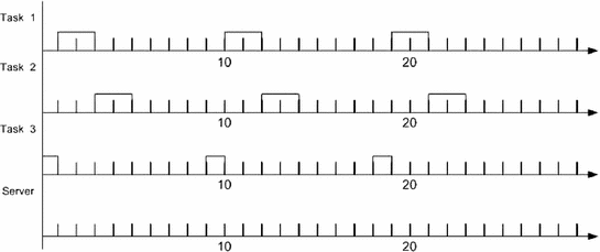
Task ordering using a PE algorithm
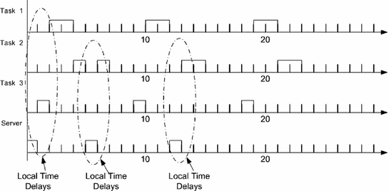
Tiny time delays for two scenarios
These two scenarios present two different local time delays that need to be taken into account beforehand, in order to settle the related delays, according to scheduling approach and control design. These time delays can be expressed in terms of local relations among dynamical systems. These relations are the actual and possible time delays, bounded as marked by a limit of possible and current scenarios. Then, time delays may be expressed as local summations, with a high degree of certainty, for each specific scenario.
A distributed system is loosely coupled, and thus, it has a high cost to know its global state, given the communication among its elements. The scheduling in each agent allows to achieve the time restrictions, and takes decisions that control the access to resources in an independent way; however, this may carry out decisions that, globally, are not at all certain.
In this design stage of distributed control systems, also known as NCS, it is considered as an important element of analysis to determine the range of sampling periods in which the system presents an acceptable performance.
Nowadays, the trend in systems that integrate computing, communication, and control, make use of control architectures with a common communication network. This improves the efficiency, flexibility, and reliability of distributed systems. Nevertheless, this architecture implies several kinds of time delays between sensors, controllers, and actuators, due to they share a communication media, as well as due to the communication process. Cervin et al. [100] discuss the possibility of analysing the performance of controller under the effect of modifying the sampling intervals and the time delays of communication.
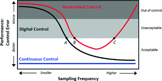
Performance comparison of continuous control, digital control, and networked control cases
(Modified from [26])
The exponential distribution is used supposing that the distance between nodes is relatively short (just a router) and the Gaussian distance for relatively long distances (multiple routers). For short distances, the time delay distributions can be divided into two parts: one constant and one variable. The constant part is defined due to the communication time delay provided by the physical length of the wiring and the processing time of the involved nodes, while the variable part is mostly affected by the stack of packages in elements such as switches and routers [99].
Having defined time delays as the result of a scheduling and networking approach, as well as external events like faults (just local and bounded faults), several scenarios are potentially presented following this time delay behaviour. In fact, the number of scenarios is finite, since the combinatorial formation is bounded as well as the kind of time delay.
 ). For computing this in the controller node, first it is obtained the sensor-controller time delay (
 ) (Eq. 1.3) and the lost packages between sensor and controller (
 ), and then, the time delay between controller and actuator is estimated (
 ), finally obtaining the estimated variable sampling period
  .
.
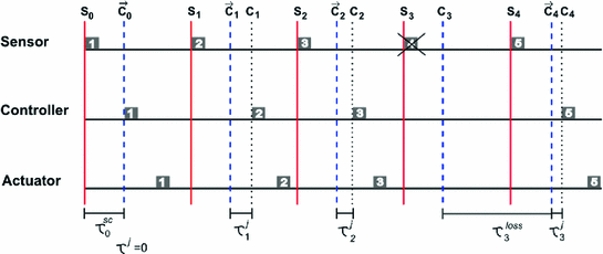
Representation of time delays during communications
 ) are used to estimate the lost packages between controller and actuator, which are measured without information for calculating the controller signal, and that modify the estimate of the time delay between controller and actuator (
 ). Supposing there is a controller node with timestamps for package arrival from the sensor (
 ) and timestamp for package emission to the sensor node (
 ):
):

 is the jitter (time delay variation) that composes the current sensor-controller time delay (
 ), along with the unknown initial time delay (
 ),
),  is the execution time of the
  controller without jitter, with
  and
and  as the timestamps of the packets in the sensor and control nodes, respectively.
  are the lost packets between sensor and controller at time i, and
  is the sampling period at time i (Fig. 1.4). Once the time delay
  of the system is estimated, it is used to generate a control signal through a fuzzy controller, as presented in Chap. 4.
1.7 Maximum Allowable Transfer Interval
Maximum Allowable Transfer Interval (MATI) is a strategy to determine certain kind of intervals in terms of transmission, which is to bound the time delay. This is possible since the source of time delays is the communication in the network. MATI has been explored in [75], giving a clear condition for the worst case scenario, but in a dynamic strategy, and guarantee limit conditions, either using Lyapunov Krasovskii strategy [101], or TSK Fuzzy control.
In [33], Walsh introduced static and dynamic scheduling policies, but just for transmission from the sensor to controller in a continuous-time Linear Time Invariant (LTI) system. They introduce the notion of MATI as the longest time in which a sensor should transmit a datum. Therefore, Walsh derived Try-Once-Discarded (TOD) scheduling where the MATI constraint ensures at least one such transmission every T seconds. However, TOD does not guarantee that each node transmits once every p transmissions. In [67], Zhang extends [33], developing a theorem that ensures the negative nature of the Lyapunov derivative function, defined for a discrete-time LTI system at each sampling instant.
Regarding NCS, [2] also analyses several important facets of NCSs, by introducing models for the delays in NCS: first as a fixed delay, then as an independently random, and finally, like a Markov process. Optimal stochastic control theorems for NCSs are introduced, based on the independently random and Markovian delay models. Koubias [102] introduced static and dynamic scheduling policies for transmission of sensor data in a continuous-time LTI system. They introduce the notion of the maximum allowable transfer interval (MATI). This is the longest time after which a sensor should transmit a data. They also derive bounds of the MATI, such that the NCS is kept stable. This MATI ensures that the Lyapunov function of the system under consideration is strictly decreasing at all times [103]. This work extends the work in [102] developing a theorem which ensures the decrease of a Lyapunov function for a discrete-time LTI system at each sampling instant, by using two different bounds. These results are less conservative than those in [33] since here it is not required that the system Lyapunov function should be strictly decreasing at all time. Further, a number of different LMI tools for analysing and designing optimal switched NCSs are introduced. Alternatively, [99] takes into consideration both the network-induced delay and the time delay in the plant, and thus, introduces a controller design method, using a delay-dependent approach.
In a NCS, the main problems that degrade NCS performance are network-induced delays and packet loss. Time delays can be constant, time-varying or even random; those depend on the scheduler, network type, architecture, operating systems, etc. [2]. When a NCS uses a reliable network, it is possible to compensate for time delays lower or larger than the sampling period and obtain bounds. However, when a NCS uses an unreliable network, it is more difficult to compensate for the time delays and packet loss, and these reduce the efficiency of NCS. Therefore, analyse time delay and packet loss to develop an efficient approach and reduce its effect is critical for NCS with an unreliable network.
Nilsson has been a pioneer, analysing several important facets of NCSs [2]. He introduced models for fixed, independently random and Markovian time delays in NCSs. His paper introduced optimal stochastic control theorems for NCSs based upon the independently random and Markovian delay models. In [33], static and dynamic scheduling policies for transmission of sensor-controller data in continuous-time, linear time-invariant (LTI) systems are reviewed. Furthermore, the notion of the MATI was introduced, which is the longest time for that a sensor transmit a data with the warranty of a stable NCS. In [104], the work of Walsh was extended. He developed a theorem, which ensures the decrease of a Lyapunov function for a discrete-time LTI system at each sampling instant, using two different bounds; in the last two cases, only the communication between the sensor and controller is provided.
1.8 Organization of the Book
This book contains seven chapters. This first chapter presents an introduction to NCS, collecting of the most common methodologies in the NCS design, also shows some fundamental concepts for the development of this book, such as the time delay modelling and the definition of a maximum bound to consider that the system is stable. Chapter 2 presents a statistical model of the time delays generated within a non-deterministic communication network. Also, three NCS models are presented to incorporate the effects of network imperfections into the design, as well as an identification model for NCS. Chapter 3 presents a brief introduction to the modelling of distributed systems, considering their dynamic behaviour based on real-time representation, such as scheduling algorithms and relationship matrices. Chapter 4 presents the NCS design for each of the models presented in Chap. 2, generating the control and scheduling laws as well as a control-scheduling codesign that improve the system performance. Chapter 5 shows some approaches for designing mobile control applications, taking into account consensus and routing algorithms for decision making, as well as the delays generated by the makings decision. Chapter 6 provides two cases studies that are used to apply the control, scheduling and codesign methodologies presented throughout the previous chapters, providing the details of the effects of time delays, as well as the proper NCS design for each one of the challenging experimental benchmarks. Finally, Chap. 7 provides a summary of the contents of all previous chapters, in the form of a conclusion, and some aims for future work.