Chapter 4

Grabbing Data from External Sources

IN THIS CHAPTER

Understanding external data sources

Exporting data from other programs

Importing data into Excel

Grabbing data from the web

Querying an external database

In many cases, the data that you want to analyze resides outside Excel. That data could be in a text file or a Word document, on a web page, in a database file, in a database program, such as a corporate accounting system, or on a special database server. Alas, you can’t analyze anything that’s hunkered down “out there” in a file, a program, or a server. Instead, you’ve got to figure out a way to get that data “in here,” by which I mean that you import that data into an Excel workbook and in the form of an Excel table. Importing can be quite a challenge, but fortunately, Excel offers many powerful tools for importing outside data.

You can use two basic approaches to grabbing the external data that you want to analyze. You can export data from another program and then import that data into Excel, or you can query a database directly from Excel. I describe both approaches in this chapter.

What’s All This About External Data?

A vast amount of data exists in the world, and most of it resides in some kind of nonworkbook format. Some data exists in simple text files, perhaps as comma-separated lists of items. Other data resides in tables, either in Word documents or, more likely, Access databases. Also, an increasing amount of data is available on web pages. External data is data that resides outside Excel in a file, database, server, or website.

By definition, external data is not directly available to you via Excel. However, Excel offers a number of tools that enable you to import external data into the program, and from there you can break out Excel’s data-analysis tools to extract useful information from that data.

The world’s data exists in a seemingly endless variety of files and formats. Here are some of the external data types you’re most likely to come across:

• Access table: Microsoft Access is the Office suite’s relational database management system. It’s often used to store and manage the bulk of the data used by a person, team, department, or company. You can connect to Access tables either via Excel’s Query Wizard or by importing table data directly into Excel.
• Word table: Simple collections of data are often stored in a table embedded in a Word document. You can perform only so much analysis on that data within Word, so importing the data from the Word table into an Excel worksheet is often useful.
• Text file: Text files often contain useful data. If that data is formatted properly — for example, each line has the same number of items, all separated by spaces, commas, or tabs — you can import that data into Excel for further analysis.
• Web page: People and companies often make useful data available on web pages that reside either on the Internet or on company networks. This data is often a combination of text and tables, but you can’t analyze web-based data in any meaningful way in your web browser. Fortunately, Excel enables you to create a web query that lets you import text and tables from a web page.
• XML file: XML (Extensible Markup Language) is a special text format for storing data in a machine-readable format.
• External programs and services: Many programs store data: accounting and finance systems; contact management programs; inventory control software; and on and on. The bad news is that for the vast majority of such programs, Excel has no way to import the program’s data directly. The good news is that Excel is so popular that many programs that store data also include a feature that lets you export the data as an Excel workbook. Even those programs that don’t offer a way to save data as a workbook do offer techniques for exporting the data to other formats that Excel can work with, such as text or XML files.

Exporting Data from Other Programs

Before getting to the techniques for importing data into Excel, take a minute to consider how you might export data from an external program into a format that Excel can use. Fortunately, most programs that store data also offer a (usually) straightforward way to export data. Even better, because Excel is the dominant data-analysis tool available to business, you can almost always tweak a program’s export routine to produce data in an Excel-friendly format.

What does it mean for exported data to be Excel friendly? It means that the resulting data is in one of the following two formats:

• Excel workbook: This is the gold standard of exporting, because it means that you don’t even need to import the data into Excel. Instead, you just open the workbook and start analyzing the data (although you might need to convert the data into a table as a first step).
• An external file that Excel can import: In most cases, this means a text file or an XML file.

Therefore, when exporting data from some other program, your first step is to do a little bit of digging to see whether you have a way to easily and automatically export data to Excel. This fact-finding shouldn't take much time if you use the program’s Help system. Next, you need to find the program’s Export feature. You can usually find the Export command on the File menu, although you might first need to open a submenu with a name such as Import/Export, Save As, or Utilities. After you’ve launched the export process, look for an option to save the data directly to an Excel workbook. If you don’t see an Excel option, say “Aw, too bad!” and look for a way to export the data as a text file or XML file. If you go the text file route, be sure to export the data using one of the following two formats:

• Delimited text file: Uses a structure in which each item on a line of text is separated by a character called a delimiter. The most common text delimiter is the comma (,) and such a file is known as a comma-separated values (CSV) file. When Excel imports a delimited text file, it treats each line of text as a record and each item between the delimiter as a field.
• Fixed-width text file: Uses a structure in which all the items use a set amount of space — for example, one item might always use 10 characters, whereas another might always use 20 characters — and these fixed widths are the same on every line of text. Excel imports a fixed-width text file by treating each line of text as a record and each fixed-width item as a field.

With your external data in a format that Excel can work with, you’re ready to get that data imported into Excel.

Importing External Data into Excel

After you have access to the data, your next step is to import it into an Excel worksheet for analysis and manipulation. Depending on the amount of data, this can make your worksheet quite large. However, having direct access to the data gives you maximum flexibility when it comes to analyzing the data. Not only can you use Excel’s main data-analysis tools — tables, scenarios, and what-if analysis — but you can also create a PivotTable from the imported data. I talk about powerful PivotTables in Part 2, “Analyzing Data with PivotTables and PivotCharts.”

The next few sections take you through the specifics of importing various data types into Excel.

Importing data from an Access table

If you want to use Excel to analyze data from a table or query within an Access database, you can import the table or query into an Excel worksheet. You can use the Query Wizard (described later in this chapter) to perform this task. However, if you don’t need to filter or sort the data before importing it, you can import the table or query directly from the Access database, which is usually a bit faster. Here are the steps to follow to import a table or query directly from Access:

1. (Optional) If you want the imported data to appear in an existing worksheet, select the cell that you want Excel to use as the upper-left corner of the destination range.

2. Choose Data ⇒ Get Data ⇒ From Database ⇒ From Microsoft Access Database.

   The Import Data dialog box appears.

3. Open the folder that contains the database, select the Access database file, and then click Import.

   Excel analyzes the Access database and then displays a window that lists the tables and queries that are available to import.

   Alternatively, you might see message similar to The database has been place in a state by user ‘Whoever’ on machine ‘Whatever’ that prevents it from being opened or locked. Yikes! This means that someone else is using the database right now, so you should try again later.

4. Use the Navigator pane to select the table or query you want to import.

   A preview of the data appears, as shown in Figure 4-1.

5. Tell Excel where you want the imported data to appear by choosing Load ⇒ Load To and then selecting one of the following:
   • Existing Worksheet: Imports the data starting at the cell you selected in Step 1. If you decide that you prefer a different cell, use the range box below this option to select where you want the imported data to begin.
   • New Worksheet: Imports the data into a new worksheet. Note that this is the default import, so you can import the data directly to a new worksheet by selecting the Load button instead of dropping down the Load list.

6. Select OK.

   Excel imports the Access data into the worksheet.

FIGURE 4-1: Select a table or query in the Navigator pane to see a preview of the data.

Importing data from a Word table

A Microsoft Word table is a collection of rows, columns, and cells, which means that it looks something like an Excel range. Moreover, you can insert fields into Word table cells to perform calculations. These fields support cell references, built-in functions, and operators. Cell references designate specific cells; for example, a reference such as B1 refers to the cell in the second column and first row of the table. You can use cell references with built-in functions such as SUM and AVERAGE, and operators such as addition (+), multiplication (*), and greater than (>), to build formulas that calculate results based on the table data.

However, Excel still offers far more sophisticated data-analysis tools. Therefore, to analyze your Word table data properly, you should import the table into an Excel worksheet. Here are the steps to trudge through:

1. Launch Microsoft Word and open the document that contains the table.

2. Select a cell inside the table you want to import.

   Excel adds the Table Tools contextual tab to the ribbon.

3. Under the Table Tools contextual tab, choose Layout ⇒ Select ⇒ Select Table.

   You can also select the table by selecting the table selection handle, which appears in the upper-left corner of the table.

4. Choose Home ⇒ Copy or press Ctrl+C.
5. Switch to the Excel workbook into which you want to import the table.
6. Select the cell where you want the table to appear.

7. Paste the table data.

   How you paste the table depends on whether you want Excel to create a link with the original Word table:

   • If you don't want any connection between Excel and the original Word table, choose Home ⇒ Paste or press Ctrl+V. This means that if you make changes to the Word data, those changes aren’t reflected in the Excel data (and vice versa).
   • If you want any changes made to the original Word table to be reflected in the pasted Excel range, choose Home ⇒ Paste  ⇒ Paste Special. In the Paste Special dialog box, select the Paste Link radio button, select HTML in the As list, and then click OK. The resulting Excel range is linked to the original Word data, which means that any changes you make to the data in Word automatically appear in the Excel range. Sweet! However, you can’t change the data in Excel.

Introducing text file importing

Nowadays, most data reside in some kind of special format: an Excel workbook, an Access database, a server database, a web page, and so on. However, finding data stored in simple text files is still relatively common because text is a universal format that users can work with on any system and in a wide variety of programs. You can analyze the data contained in certain text files by importing the data into an Excel worksheet. Note, however, that you cannot import just any text file into Excel; the file needs to use either the delimited or fixed-width format.

Importing a delimited text file

A delimited text file uses a structure in which each item on a line of text is separated by a character called a delimiter. The most common text delimiter is the comma (,), and the resulting file is called a comma-separated values (or CSV) file. When Excel imports a delimited text file, it treats each line of text as a row (record) and each item between the delimiter as a column (field).

Follow these steps to import a delimited text file into Excel:

1. (Optional) To import the data to a specific location in an existing worksheet, select the cell that you want to use as the upper-left corner of the destination range.

2. Choose Data ⇒ From Text/CSV (or, if you want the workout, choose Data ⇒ Get Data ⇒ From File ⇒ From Text/CSV).

   The Import Data dialog box appears.

3. Open the folder that contains the text file, select the file, and then click Import.

   Excel analyzes the file and then opens a window that displays a preview of the data in the file.

4. In the Delimiter list, select the delimiter character that your text data uses.

   How do you know which delimiter character to choose? The comma is by far the most common delimiter, so start with that. You’ll know you’ve hit the delimiter jackpot when the previewed data appears in separate columns, as shown in Figure 4-2.

5. Either choose Load to import the data into a new worksheet or choose Load ⇒ Load To ⇒ Existing Worksheet ⇒ OK to import the data starting at the cell you selected in Step 1.

   Excel imports the delimited text data into the worksheet.

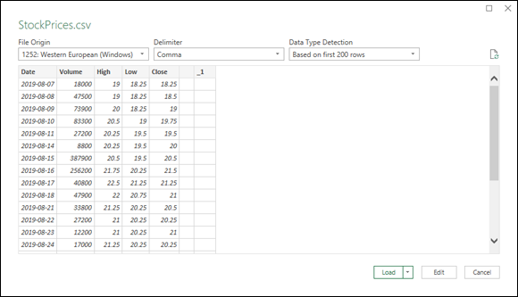
FIGURE 4-2: Select the delimiter that gets the data into nice, neat columns.

Importing a fixed-width text file

A fixed-width text file uses a structure in which all the items use a set amount of space. The first item might always be, say, 10 characters wide (including spaces); the second item might always be 8 characters wide; and so on. Crucially, these fixed widths are the same on every line of text, which gives the entire file a predictable and regular structure that Excel can work with. Excel imports a fixed-width text file by treating each line of text as a row (record) and each fixed-width item as a column (field).

If you’re importing data that uses the fixed-width structure, you need to tell Excel where the separation between each field occurs. In a fixed-width text file, each column of data is a constant width, and Excel is usually quite good at determining these widths. So in most cases, Excel automatically sets up column break lines, which are vertical lines that separate one field from the next. However, titles or introductory text at the beginning of the file can impair the wizard’s calculations, so you should check carefully that the proposed break lines are accurate.

Follow these steps to import a fixed-width text file into Excel:

1. (Optional) To load the data into a specific worksheet location, select the cell that you want to use as the upper-left corner of the destination range.

2. Choose Data ⇒ From Text/CSV (or, if you have extra time to kill, choose Data ⇒ Get Data ⇒ From File ⇒ From Text/CSV).

   The Import Data dialog box appears.

3. Open the folder that contains the text file, select the file, and then click Import.

   Excel analyzes the file and then opens a window that displays a preview of the data in the file.

4. In the Delimiter list, make sure that the Fixed Width item is selected.

   Below the Delimiter list, Excel displays a series of numbers, each of which represents the starting point of a column in the text file. The first column always starts at 0, and each subsequent value depends on the width of each column. Figure 4-3 shows these values as 0, 30, 45.

5. If your columns look incorrect — for example, one or more columns are too large or too small — edit the column starting-point values until the columns are correct, as shown in Figure 4-3.

6. Either choose Load to import the data into a new worksheet or choose Load ⇒ Load To ⇒ Existing Worksheet ⇒ OK to import the data starting at the cell you selected in Step 1.

   Excel imports the fixed-width text data into the worksheet.

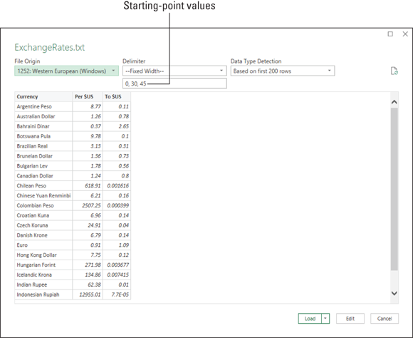
FIGURE 4-3: If needed, edit the column starting points until your columns are correct.

Importing data from a web page

You already know that the web is home to more information than you can ever use, but did you know that some of that data is available to import into Excel? I talk about a more sophisticated web-based data format in the next section, but here I want to introduce you to web data that comes in the form of a table. A web page table is a rectangular array of rows and columns, with data values in the cells created by the intersection of the rows and columns. Why, that sounds just like an Excel table, doesn’t it? It sure does, and that similarity means that if you know the address of the page that contains the table, Excel offers a tool that lets you import that data into a worksheet for more data-analysis fun.

Here are the steps to follow to import a web page table into Excel:

1. (Optional) To load the data into a specific worksheet location, select the cell that you want to use as the upper-left corner of the destination range.

2. Choose Data ⇒ From Web (or, if you prefer the scenic route, choose Data ⇒ Get Data ⇒ From Other Sources ⇒ From Web).

   The From Web window appears.

3. Enter the address of the web page in the URL text box and then click OK.

   Excel displays the Access Web Content dialog box.

4. Specify how you want to access the web page and then click Connect.

   As shown in Figure 4-4, Excel offers five methods that you can use to access the web content:

   • Anonymous: Accesses the content directly, without authentication (such as a username and password). This is the method to use for most web pages.
   • Windows: Accesses the content by logging in using the credentials (that is, the username and password) of your Windows account. This is the method to use if the content resides on your company’s network.
   • Basic: Accesses the content by logging in with a username and password that you provide. This is the method to use if you have an account on the website that hosts the content.
   • Web API: Accesses the content by using a unique value — called a key — to authenticate your request. This is the method to use if content is made available through a web application programming interface (API). The instructions for using the web API tell you how to obtain a key.
   • Organizational Account: Accesses the content by having you sign in to your organization’s Office 365 or OneDrive for Business account.

   Excel connects to the web content, analyzes the web page, and then opens the Navigator dialog box, which displays a list of the tables found on the page. One of these objects is always named Document, and it contains a table of data related to the entire web page (so you can safely ignore it).

5. Select the table you want to import.

   Excel displays a preview of the table, as shown in Figure 4-5. If you want to see what the table looks like on the web page, click the Web View tab.

6. (Optional) If you want to import multiple tables, select the Select Multiple Items check box and then select the check box beside each table you want to import.

7. Either choose Load to import the data into a new worksheet or choose Load ⇒ Load To ⇒ Existing Worksheet ⇒ OK to import the data starting at the cell you selected in Step 1.

   Excel imports the web table data into the worksheet.

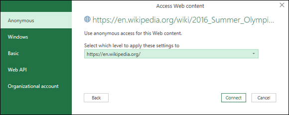
FIGURE 4-4: Choose the method you want to use to access the web data.

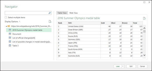
FIGURE 4-5: Select a table to preview its data.

Importing an XML file

XML (Extensible Markup Language) is a standard that enables the management and sharing of structured data using simple text files. These XML files organize data using tags, among other elements, that specify the equivalent of a table name and field names. Here’s an example that shows the first few records in an XML table of book info:

<?xml version="1.0"?>
<catalog>
<book>
<author>Gambardella, Matthew</author>
<title>XML Developer's Guide</title>
<genre>Computer</genre>
<price>44.95</price>
<publish_date>2000-10-01</publish_date>
<description>An in-depth look at creating applications
with XML.</description>
</book>
<book>
<author>Ralls, Kim</author>
<title>Midnight Rain</title>
<genre>Fantasy</genre>
<price>5.95</price>
<publish_date>2000-12-16</publish_date>
<description>A former architect battles corporate zombies,
an evil sorceress, and her own childhood to become queen
of the world.</description>
</book>
<book>
<author>Corets, Eva</author>
<title>Maeve Ascendant</title>
<genre>Fantasy</genre>
<price>5.95</price>
<publish_date>2000-11-17</publish_date>
<description>After the collapse of a nanotechnology
society in England, the young survivors lay the
foundation for a new society.</description>
</book>
etc.
</catalog>

Because XML is just text, if you want to perform data analysis on the XML file, you must import the file into an Excel worksheet. Excel stores imported XML data in an Excel table.

Here are the steps to follow to import an XML file into an Excel worksheet:

1. (Optional) To import the data to a specific location in an existing worksheet, select the cell that you want to use as the upper-left corner of the destination range.

2. Choose Data ⇒ Get Data ⇒ From File ⇒ From XML.

   The Import Data dialog box appears.

3. Open the folder that contains the XML file, select the file, and then click Import.

   Excel analyzes the XML file and then opens the Navigator dialog box, which displays a list of the tables found in the file.

4. Select the table you want to import.

   Excel displays a preview of the table, as shown in Figure 4-6.

5. (Optional) If you want to import multiple XML tables, select the Select Multiple Items check box and then select the check box beside each table you want to import.

6. Either choose Load to import the data into a new worksheet or choose Load ⇒ Load To ⇒ Existing Worksheet ⇒ OK to import the data starting at the cell you selected in Step 1.

   Excel imports the XML data into the worksheet.

FIGURE 4-6: Select an XML table to preview its data.

Querying External Databases

If you want to analyze data using a sorted, filtered subset of an external data source, Excel offers the Query Wizard tool, which enables you to specify the sorting and filtering options and the subset of the source data that you want to work with. Why bother doing all that work? Because databases such as those used in Microsoft Access and SQL Server are often very large indeed and contain a wide variety of data scattered over many different tables.

With data analysis, you rarely use an entire database as the source. Instead, you extract a subset of the database: a table, or perhaps two or three related tables. You might also require the data to be sorted in a certain way, and perhaps need to filter the data so that you work with only certain records. The specifics of these three operations — extracting a subset, sorting, and filtering — constitute the criteria for the data you want to work with, and all together they make up what’s known in the trade as a database query.

Defining a data source

All database queries require two things at the very beginning: access to a database and an Open Database Connectivity, or ODBC, data source for the database. ODBC is a database standard that enables a program to connect to and manipulate a data source. An ODBC data source contains three things: a pointer to the file or server where the database resides; a driver that enables the Query Wizard to connect to, manipulate, and return data from the database; and optional login information that you require to access the database.

Before you can do any work with the Query Wizard, you must select the data source that you want to use. If you have a particular database that you want to query, you can define a new data source that points to the appropriate file or server.

Most data sources point to database files. For example, the relational database management program Microsoft Access uses file-based databases. You can also create data sources based on text files and Excel workbooks. However, some data sources point to server-based databases. For example, SQL Server and Oracle run their databases on special servers. As part of the data source definition, you need to include the software driver that the Query Wizard uses to communicate with the database, as well as any information that you require to access the database.

Follow these steps to define a data source for your query:

1. Choose Data ⇒ Get Data ⇒ From Other Sources ⇒ From Microsoft Query.

   The Choose Data Source dialog box appears, as shown in Figure 4-7.

   Your computer probably comes with a few predefined data sources that you can use instead of creating new ones. In the Choose Data Source dialog box, any predefined data sources appear in the Databases tab. For example, Microsoft Office creates two default data sources: Excel Files and MS Access Database. These incomplete data sources don’t point to a specific file. Instead, when you select one of these data sources and then click OK, Excel prompts you for the name and location of the file. These data sources are useful if you often switch the files that you’re using. However, if you want a data source that always points to a specific file, you need to follow the steps in this section.

2. Choose <New Data Source>, deselect the Use the Query Wizard to Create/Edit Queries check box, and then click OK.

   The Create New Data Source dialog box appears.

3. In the What Name Do You Want to Give Your Data Source? text box, enter a name for your data source.

   This name appears in the Databases tab of the Choose Data Source dialog box, so enter a name that helps you remember which data source you’re working with.

4. From the Select a Driver for the Type of Database You Want to Access list, select the database driver that your data source requires.

   For example, for an Access database, select Microsoft Access Driver (*.mdb, *.accdb).

   Many businesses store their data in Microsoft SQL Server databases (SQL is usually pronounced ess-kew-ell). This is a powerful server-based system that can handle the largest databases and thousands of users. To define an SQL Server data source, select SQL Server. Click Connect to display the SQL Server Login dialog box. Ask your SQL Server database administrator for the information you require to complete this dialog box. Type the name or remote address of the SQL Server in the Server text box, type your SQL Server login ID and password, and then click OK. Perform Steps 9 and 10 later in this section to complete the data source.

5. Click Connect.

   The dialog box for the database driver appears. The steps that follow show you how to set up a data source for a Microsoft Access database.

6. Click the Select button.

   The Select Database dialog box appears.

7. Open the folder that contains the database, select the database file, and then click OK.

   Excel returns you to the database driver’s dialog box.

   If you use a login name and password to access the database, click Advanced to display the Set Advanced Options dialog box. Type the login name and password and then click OK.

8. Click OK.

   Excel returns you to the Create New Data Source dialog box. Figure 4-8 shows the completed dialog box for the Northwind Access database that I’m using.

   You can use the Select a Default Table for Your Data Source list to select a table from the database. When you do this, each time you start a new query based on this data source, the Query Wizard automatically adds the default table to the query, thus saving you several steps.

   If you specified a login name and password as part of the data source, you can select the Save My User ID and Password in the Data Source Definition check box to save the login data.

9. Click OK.

   Excel returns to the Choose Data Source dialog box, which now displays your shiny, new data source.

10. Click Cancel to bypass the steps for importing the data.

    You can now use the data source in the Query Wizard, which I talk about in the next section.

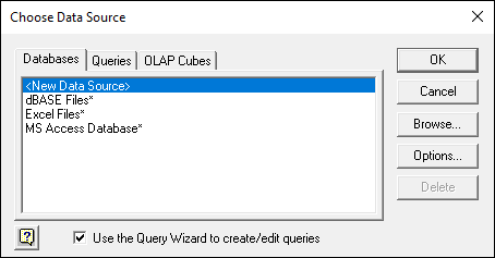
FIGURE 4-7: The Choose Data Source dialog box.

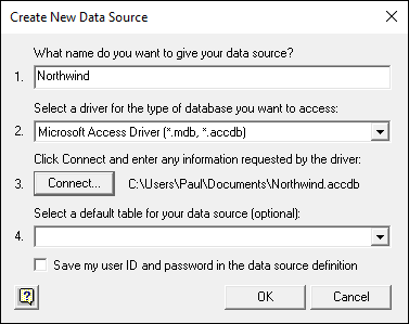
FIGURE 4-8: The completed Create New Data Source dialog box for the Northwind database.

Querying a data source

To run a database query and import the query results, follow these steps:

1. Choose Data ⇒ Get Data ⇒ From Other Sources ⇒ From Microsoft Query.

   Excel displays the Choose Data Source dialog box. In Figure 4-9, you can see that the Northwind data source I created in the previous section now appears in the Databases tab.

2. Select the Use the Query Wizard to Create/Edit Queries check box.

   If you didn’t define a new data source as described in the previous section, this check box should already be selected for you.

3. On the Databases tab, select the database you want to query and then click OK.

   If you choose one of the predefined database types, Excel displays the Select Database dialog box. In this dialog box, select the database that you want to query and then click OK.

   Excel displays the Query Wizard - Choose Columns dialog box.

   You use the Query Wizard - Choose Columns dialog box to pick which tables and which table columns (fields) you want to appear in your query results. In the Available Tables and Columns box, Excel lists tables and columns. Initially, this list shows only tables, but you can see the columns within a table by clicking the + icon next to the table name.

4. Populate the Columns in Your Query list with the columns you want to work with.

   You have three techniques to use:

   • To add an entire table to the list, click the table name and then click the right-facing arrow button that points to the Columns in Your Query list box.
   • To add a single column from a table to the list, click the + icon beside the table name, select the column, and then click the right-facing arrow button that points to the Columns in Your Query list box.
   • To remove a column, select the column in the Columns in Your Query list box and then click the left-facing arrow button that points to the Available Tables and Columns list box.

   This all sounds very complicated, but it really isn’t. Essentially, all you do is identify the columns of information that you want in your Excel table. Figure 4-10 shows how the Query Wizard - Choose Columns dialog box looks after adding several columns from the Products table and one column (CategoryName) from the Categories table.

5. After you identify which columns you want in your query, click the Next button to filter the query data.

   Excel displays the Query Wizard - Filter Data dialog box.

   You can filter the data returned as part of your query by using the Only Include Rows Where text boxes. For example, to include only rows in which the CategoryName column equals Beverages, click the CategoryName column in the Column to Filter list box. Then select the Equals filtering operation from the first drop-down list and enter the value Beverages into the second drop-down list (or select it); you can see this filter in action in Figure 4-11.

   The Query Wizard - Filter Data dialog box performs the same sorts of filtering that you can perform with the AutoFilter command and the Advanced Filter command. Because I discuss these tools in Chapter 3, I don't repeat that discussion here. However, note that you can perform quite sophisticated filtering as part of your query.

6. (Optional) Filter your data based on multiple filters by selecting the And or Or radio buttons.
   • And: A row is included in the query only if it matches all the filter conditions.
   • Or: A row is included in the query if it matches one or more of the filter conditions.

7. Click Next.

   Excel displays the Query Wizard - Sort Order dialog box.

8. Choose a sort order for the query result data from the Query Wizard - Sort Order dialog box.

   Select the column that you want to use for sorting from the Sort By drop-down list and then select one of the following radio buttons (see Figure 4-12):

   • Ascending: The column values are sorted in increasing order: A to Z if the column contains text, 0 to 9 for numbers, earlier to later for dates or times.
   • Descending: The column values are sorted in decreasing order: Z to A for text, 9 to 0 for numbers, later to earlier for dates or times.

   You can also use additional sort keys by selecting fields in one or more of the Then By drop-down lists that appear in the Query Wizard – Sort Order dialog box. The wizard displays enough drop-down lists for every field in your query.

   You sort query results the same way that you sort rows in an Excel table. If you have more questions about how to sort rows, refer to Chapter 3. Sorting works the same whether you’re talking about query results or rows in a table.

9. Click Next.

   Excel displays the Query Wizard - Finish dialog box.

10. In the Query Wizard - Finish dialog box, specify where Excel should place the query results.

    For most types of data, you have two choices:

    • Return Data to Microsoft Excel: Sends the data to Excel without further review on your part.
    • View Data or Edit Query on Microsoft Query: Opens the query in a separate Office program called Microsoft Query. This is a sophisticated database query program, the workings of which are beyond the scope of this book. If you decide to try this program, when you’re finished with it, choose File ⇒ Return Data to Microsoft Excel and then continue with Step 12.

11. Click the Finish button.

    After you click the Finish button to complete the Query Wizard, Excel displays the Import Data dialog box.

12. In the Import Data dialog box, choose the worksheet location for the query result data.

    Use this dialog box to specify where query-result data should be placed.

    • To place the query-result data in an existing worksheet, select the Existing Worksheet radio button. Then identify the cell in the top-left corner of the worksheet range and enter its location in the Existing Worksheet text box.
    • Alternatively, to place the data into a new worksheet, select the New Worksheet radio button.

13. Click OK.

    Excel places the data at the location that you chose.

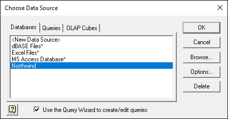
FIGURE 4-9: Any data sources that you’ve created appear in the Databases tab.

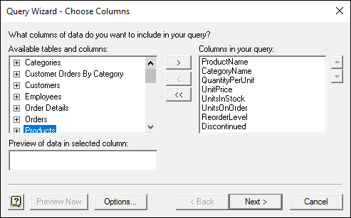
FIGURE 4-10: The completed Query Wizard – Choose Columns dialog box.

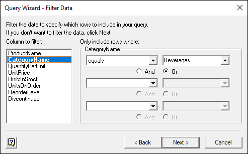
FIGURE 4-11: The Query Wizard – Filter Data dialog box with a filter added.

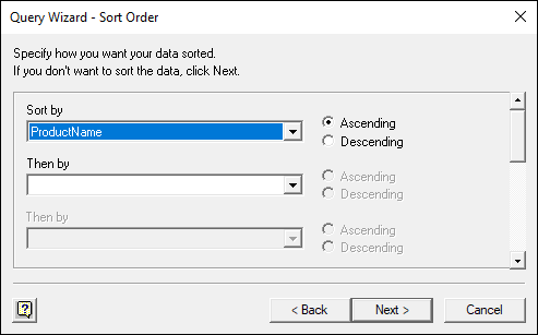
FIGURE 4-12: The Query Wizard – Sort Order dialog box.

It's Sometimes a Raw Deal

By using the instructions that I describe in this chapter to retrieve data from some external source, you can probably get the data rather quickly into an Excel workbook. But you may have also found that the data is rather raw and are saying to yourself (as I would be, in your shoes), “Wow, this stuff is pretty raw.”

But don't worry: You are where you need to be. Having your information be raw at this point is okay. In Chapter 5, I discuss how you clean up the workbook by eliminating rows and columns and information that are not part of your data. I also cover how you scrub and rearrange the actual data in your workbook so that it appears in a format and structure that’s useful to you in your upcoming analysis.

The bottom line is this: Don't worry that your data seems a bit ugly right now. Getting your data into a workbook accomplishes an important step. Now you need to spend a little time on your housekeeping. Read through the next chapter for the lowdown on how to do that.

By the way, if the process of importing data from some external source has resulted in very clean and pristine data — and this might be the case if you've grabbed data from a well-designed database or with help from the corporate database administrator — that's great. You can jump right into the data-analysis techniques that I start describing in Chapter 6.