Chapter 2
Concepts of magnetic resonance

In its most basic form, the MR experiment can be analyzed in terms of energy transfer. During the measurement process, the patient or sample is exposed to energy at the correct frequency that will be absorbed. A short time later, this energy is reemitted, at which time it can be detected and processed. A detailed presentation of the processes involved in this absorption and reemission requires the use of linear response theory, which is beyond the scope of this book. However, a general description of the nature of the molecular interactions is useful. In particular, the relationship between the molecular picture and the macroscopic picture provides an avenue for explanation of the principles of MR.

2.1 Radiofrequency excitation

Chapter 1 described the formation of the net magnetization, M₀, by the protons within a sample. The entire field of MR is based on the manipulation of M₀. The simplest manipulation involves the application of a short burst, or pulse, of radiofrequency (RF) energy. This pulse, referred to as an excitation pulse, typically contains a narrow range or bandwidth of frequencies centered around a central frequency. During the pulse, the protons absorb a portion of this energy at a particular frequency. The particular frequency absorbed is proportional to the magnetic field B₀; the equation relating the two is the Larmor equation, equation (1.1). Following the pulse, the protons reemit the energy at the same frequency.

The frequency of energy absorbed by an individual proton is defined very precisely by the magnetic field that the proton experiences due to the quantized nature of the spin orientation. When a proton is irradiated with energy of the correct frequency (ω₀), it is excited from the lower energy (spin up) orientation to the higher energy (spin down) orientation (Figure 2.1). At the same time, a proton in the higher energy level is stimulated to release its energy and will go to the lower energy level. The energy difference (ΔE) between the two levels is exactly proportional to the frequency ω₀ and thus the magnetic field B₀:

2.1

where h is Planck's constant, 6.626 × 10⁻³⁴ Js. Only energy at this frequency stimulates transitions between the spin up and spin down energy levels. This quantized energy absorption is known as resonance absorption and the associated frequency is known as the resonant frequency.

Figure 2.1 Energy absorption (microscopic). The difference in energy ΔE between the two configurations (spin up and spin down) is proportional to the magnetic field strength B₀ and the corresponding precessional frequency ω₀, as expressed in Equation (2.1). When energy at this frequency is applied, a spin from the lower-energy state is excited to the upper-energy state. Also, a spin from the upper-energy state is stimulated to give up its energy and relax to the lower-energy state. Because there are more spins in the lower-energy state, there is a net absorption of energy by the spins in the sample.

Although an individual proton absorbs the radiofrequency energy, it is more useful to discuss the resonance condition by examining the effect of the energy absorption on M₀. For a large collection of protons such as in a volume of tissue, there is a significant amount of both absorption and emission occurring during the RF pulse. However, because there are more protons in the lower energy level (Figure 2.1), there will be a net absorption of energy by the tissue. The energy is applied as an RF pulse with a central frequency ω_TR and an orientation perpendicular to B₀, as indicated by an effective field B₁ (Figure 2.2). This orientation difference allows a coupling between the RF pulse and M₀ so that energy can be transferred to the protons. When the transmitter frequency matches the resonant frequency (ω₀ = ω_TR), the RF energy will be absorbed, which causes M₀ to rotate away from its equilibrium orientation. The initial direction of rotation of M₀ is perpendicular to both B₀ and B₁. If the transmitter is left on long enough and at a high enough amplitude, the absorbed energy causes M₀ to rotate entirely into the transverse plane, a result known as a 90° pulse. When viewed in the rotating frame, the motion of M₀ is a simple vector rotation; however, the end result is the same whether a rotating or stationary frame of reference is used.

Figure 2.2 Energy absorption (macroscopic). In a rotating frame of reference, the RF pulse broadcast at the resonant frequency ω₀ can be treated as an additional magnetic field B₁ oriented perpendicular to B₀. When energy is applied at the appropriate frequency, the spins absorb it and M rotates into the transverse plane. The initial direction of rotation is perpendicular to both B₀ and B₁. The amount of resulting rotation of M is known as the pulse flip angle.

2.2 Radiofrequency signal detection

When the transmitter is turned off, the protons immediately begin to realign themselves and return to their original equilibrium orientation. They emit energy at frequency ω₀ as they do so. In addition, the net magnetization will begin to precess about B₀ similar to the behavior of a gyroscope when tilted away from a vertical axis. If a loop of wire (receiver) is placed perpendicular to the transverse plane, M₀ will induce a voltage in the wire during its precession. This induced voltage, the MR signal, is known as the FID, or free induction decay (Figure 2.3a). The initial magnitude of the FID signal depends on the value of M₀ immediately prior to the 90° pulse. The FID decays with time as more of the protons give up their absorbed energy through a process known as relaxation (see Chapter 3) and the coherence or uniformity of the proton motion is lost.

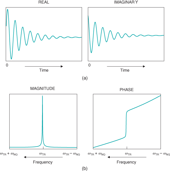
nfg003 — **Figure 2.3** (a) Free induction decay, real and imaginary. The response of the net magnetization M to an RF pulse as a function of time is known as the free induction decay (FID). Its amplitude is proportional to the amount of transverse magnetization generated by the pulse. The FID is maximized when using a 90° excitation pulse. (b) Fourier transformation of (a), magnitude and phase. The Fourier transformation is used to convert the digital version of the MR signal (FID) from a function of time to a function of frequency. Signals measured with a quadrature detector are displayed with the transmitter (reference) frequency ω_TR in the middle of the display. The Nyquist frequencies ω_NQ below and above ω_TR are the minimum and maximum frequencies of the frequency display, respectively. For historical reasons, frequencies are plotted with lower frequencies on the right side and higher frequencies on the left side of the display.

In general, three components of an MR signal are of interest: its magnitude or peak amplitude, its frequency, and its phase or direction relative to the RF transmitter phase (Figure 2.4). As mentioned previously, the signal magnitude is related to the value of M₀ immediately prior to the RF pulse. The signal frequency is related to the magnetic field influencing the protons. If all the protons experience the same magnetic field B₀, then only one frequency would be present within the FID. In reality, the magnetic field varies throughout the magnet and inside the patient, and thus the MR signal contains many frequencies varying as a function of time following the RF pulse. It is easier to examine such a multicomponent signal in terms of frequency rather than of time. The conversion of the signal amplitudes from a function of time to a function of frequency is accomplished using a mathematical operation called the Fourier transformation. In the frequency presentation or frequency domain spectrum, the MR signal is mapped according to its frequency relative to a reference frequency, typically the transmitter frequency ω_TR. For systems using quadrature detectors (see Chapter 13), ω_TR is centered in the display with frequencies higher and lower than ω_TR located to the left and right, respectively (Figure 2.3b). The frequency domain thus allows a simple way to examine the magnetic environment that a proton experiences.

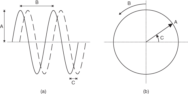
nfg004 — **Figure 2.4** Planar (a) and circular (b) representations of a time-varying wave. The amplitude (A) is the maximum deviation of the wave from its mean value. The period (B) is the time required for completion of one complete cycle of the wave. The frequency of the wave is the reciprocal of the period. The phase or phase angle of the wave (C) describes the shift in the wave relative to a reference (a second wave for the planar representation, horizontal axis for circular representation). The two plane waves displayed in (a) have the same amplitude and period (frequency) but have a phase difference of π/4, or 90°.

Since the proton precession is continuous, the MR signal is continuous or analog in nature. However, postprocessing techniques such as Fourier transformation requires a digital representation of the signal. To produce a digital version, the FID signal is measured or sampled using an analog-to-digital converter (ADC). In most instances, the resonant frequencies of protons are greater than many ADCs can process. For this reason, a phase-coherent difference signal is generated based on the frequency and phase of the input RF pulse; that is, the signal actually digitized is the measured signal relative to ω_TR. This is equivalent to examining the signal in a frame of reference rotating at ω_TR. Under normal conditions, this so-called demodulated signal is digitized for a predetermined time known as the sampling time and with a user-selectable number of data points. In such a situation, there will be a maximum frequency, known as the Nyquist frequency ω_NQ, that can be accurately measured:

2.2

In MR, the Nyquist frequency typically ranges from 500 to 500,000 Hz, depending on the combination of sampling time and number of data points. To exclude frequencies greater than the Nyquist limit from the signal, a filter known as a low pass filter is used prior to digitization. Frequencies excluded by the low pass filter are usually noise, so that filtering provides a method for improving the signal-to-noise ratio (SNR) for the measurement. The optimum SNR is usually obtained by increasing the sampling time to match the Nyquist frequency and low pass filter width for the particular measurement conditions. For quadrature detection systems typically used in MR, the total receiver bandwidth is 2 * ω_NQ centered about ω_TR (Figure 2.3b).

2.3 Chemical shift

The specific frequency that a proton absorbs is dependent on magnetic fields arising from two sources. One is the applied magnetic field B₀. The other one is molecular in origin and produces the chemical shift. In patients, the bulk of the hydrogen MR signals arise from two sources, water and fat. Water has two hydrogen atoms bonded to one oxygen atom while fat is heterogeneous in nature, with many hydrogen atoms bonded to a long chain carbon framework (typically 10–18 carbon atoms in length). Because of its different molecular environment, a water proton has a different local magnetic field than a fat proton. This local field difference is known as chemical shielding and produces a magnetic field variation that is proportional to the main magnetic field B₀:

2.3

where B_i is the magnetic field and σ_i is the shielding term for proton i. Chemical shielding produces different resonant frequencies for fat and water protons under the influence of the same main magnetic field. Because the shielding term is typically small (∼10⁻⁴–10⁻⁶), these frequency differences are very small. It is more practical to analyze the frequencies using these differences rather than using absolute terms. A convenient scale to express frequency differences is the ppm scale, which is the resonant frequency of the proton of interest relative to a reference frequency:

2.4

Frequency differences expressed in this form are known as chemical shifts. While the choice of ω_ref is arbitrary, a convenient choice is ω_TR. The primary advantage of the ppm scale is that frequency differences are independent of B₀. For fat and water, the difference in chemical shifts at all field strengths is approximately 3.5 ppm, with fat at a lower frequency. At 1.5 T, this difference is 220 Hz, while at 3.0 T, it is 450 Hz (Figure 2.5).

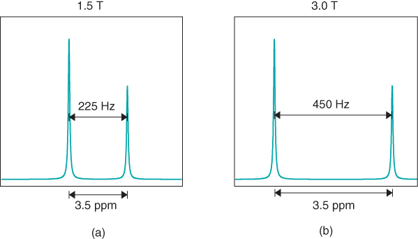
nfg005 — **Figure 2.5** Spectrum of water and fat at 1.5 T (a) and 3.0 T (b). The resonant frequencies for water and fat are separated by approximately 3.5 ppm, which corresponds to an absolute frequency difference of 220 Hz for a 1.5 T magnetic field (63 MHz) or 450 Hz at a magnetic field of 3.0 T (126 MHz).

The chemical shift difference between fat and water can be visualized in the rotating frame. A 150 Hz difference in frequency means that the fat resonance precesses slower than the water resonance by 6.7 ms per cycle (1/150 Hz). The fat resonance will align with or be in phase with the water resonance every 6.7 ms at 1.0 T. For a 1.5 T MR system, the same cycling will occur every 4.5 ms (1/220 Hz) and every 2.25 ms for a 3.0 T system (Figure 2.6). The 3.5 ppm chemical shift difference mentioned previously is an approximate difference. The fat resonance signal is a composite from all the protons within the fat molecule. The particular chemical composition (e.g., saturated versus unsaturated hydrocarbon chain, length of hydrocarbon chain) determines the exact resonant frequency for this composite signal. The 3.5 ppm difference applies to the majority of fatty tissues found in the body. Chemical shift differences between protons in different molecular environments provide the basis for MR spectroscopy, which is described in more detail in Chapter 13.

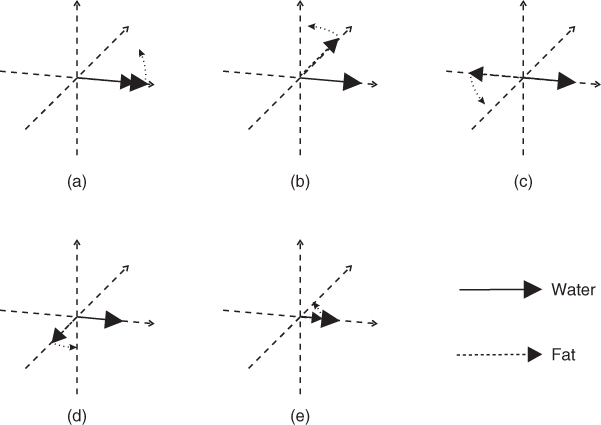
nfg006 — **Figure 2.6** Precession of fat and water protons. Because of the 3.5 ppm frequency difference, a fat proton precesses at a slower frequency than does a water proton. In a rotating frame at the water resonant frequency, the fat proton cycles in and out of phase with the water proton. Following the excitation pulse, the two protons are in phase (a). After a short time, they will be 90° out of phase (b), then 180° out of phase (c, also called “opposed phase”). Then −90° out of phase (d) and back in phase (e). The contribution of fat to the total signal fluctuates and depends on when the signal is detected. At 1.5 T, the in-phase times are 0 ms (a), 4.5 ms (e), 9 ms and so on (not shown), while the opposed-phase times are 2.25 ms (c), 6.7 ms and so on (not shown). At 3.0 T, the times are one half of the times at 1.5 T.