Chapter 4
Principles of magnetic resonance imaging – 1

Chapter 2 described the relationship between the frequency of energy that a proton absorbs and the magnetic field strength that it experiences. MRI uses this field dependence to localize these proton frequencies to different regions of space. This idea of using the field dependence to spatially localize the protons earned the 2003 Nobel Prize in Physiology or Medicine for Paul Lauterbur and Sir Peter Mansfield, and helped transform MR from a niche industry serving research labs into a multibillion-dollar industry serving hospitals worldwide.

4.1 Gradient fields

In MRI, the magnetic field is made spatially dependent through the application of magnetic field gradients. These gradients are relatively small perturbations superimposed on the main magnetic field , with a typical imaging gradient producing a total field variation of less than 1%. They are also linear perturbations to , so that the exact magnetic field is linearly dependent on the location inside the magnet:

4.1

where is the magnetic field at location and is the total gradient amplitude, mathematically represented as a tensor. Gradients are also applied for short periods of time during a scan and are referred to as gradient pulses.

---

In clinical MRI, the magnetic field gradients that are used produce linear variations primarily in one direction only, so that the tensor product in equation 4.1 can be reduced to a vector representation. Each gradient is centered around a point in the center of the magnet known as an isocenter. Variations to one side of the isocenter will have total magnetic field values greater than that at the isocenter while locations on the other side will have less than . The gradient amplitude is the slope of the line, as illustrated in Figure 4.1.

Figure 4.1 A gradient is a linear distortion of the primary magnetic field, centered at the magnet isocenter. A 40 mT m⁻¹ gradient superimposed on a 1.5 T magnet field will produce a total magnetic field variation of 1480 to 1520 mT. For a 500 mm distance, the variation will be 1490 to 1510 mT.

In the direction perpendicular or normal to the gradient, will be constant. In other words, the presence of a gradient will produce planes of constant , with the value of variation dependent on its location. The direction of variation is perpendicular or normal to the surface of the plane. Three physical gradients are used, one in each of the , and directions. Each one is assigned, through the operating software, to one or more of the three “logical” or functional gradients required to obtain an image: slice selection, readout or frequency encoding, and phase encoding. The particular pairing of physical and logical gradients is somewhat arbitrary and depends on the acquisition parameters and patient positioning as well as the choice of physical directions by the manufacturer. The only requirement is that the three logical directions must be mutually perpendicular. The combination of gradient pulses, RF pulses, data sampling periods, and the timing between each of them that are used to acquire an image is known as a pulse sequence.

---

The presence of linear magnetic field gradients requires an expanded version of the Larmor equation given in equation (1.1):

4.2

where is the frequency of the proton at position and is a vector representing the total gradient amplitude and direction. The units of measure for are expressed in millitesla per meter or gauss per centimeter , where . Equation 4.2 states that, in the presence of a gradient field, each proton will resonate at a unique frequency that depends on its exact position within the gradient field. The MR image is simply a frequency and phase map of the protons generated by unique magnetic fields at each point throughout the image. The displayed image consists of digital picture elements (pixels) that represent volume elements (voxels) of tissue. The pixel intensity is related to the number of protons contained within the voxel weighted by the tissue characteristics, like T1 and T2 relaxation times, for the tissues within the voxel according to the pulse sequence utilized.

4.2 Slice selection

---

The initial step in MRI is the localization of the RF excitation to a region of space, which is accomplished through the use of frequency-selective excitation in conjunction with a gradient known as the slice selection gradient, . The gradient direction ( or a combination) determines the slice orientation while the gradient amplitude together with certain RF pulse characteristics determine both the slice thickness and slice position. A frequency-selective RF pulse has two key features: a central frequency and a narrow range or bandwidth of frequencies (typically 1–2 kHz) (see Chapter 5 for a more detailed description of selective pulses). When such a pulse is broadcast in the presence of the slice selection gradient, a narrow region of tissue achieves the resonance condition (equation 4.2) and absorbs the RF energy. The duration of the RF pulse and its amplitude determines the amount of resulting rotation of (e.g., 90°, 180°). The central frequency of the pulse determines the particular location excited by the pulse when the slice selection gradient is present. Different slice positions are achieved by changing the central frequency. The slice thickness is determined by the gradient amplitude and the bandwidth of frequencies incorporated into the RF pulse:

4.3

Typically, is fixed for a given pulse sequence, so that the slice thickness is changed by modifying the amplitude of (Figure 4.2). Thinner slices require larger . Once is determined by the slice thickness, the central frequency is calculated using equation 4.2 to bring the desired location into resonance. Multislice imaging, the most commonly used approach for MRI, uses the same but a unique RF pulse during excitation for each slice. The RF pulse for each slice has the same bandwidth but a different central frequency, thereby exciting a different region of tissue (Figure 4.3).

Figure 4.2 For a given range (bandwidth) of frequencies included in the RF pulse, the slice thickness desired is determined by the slice-selection gradient amplitude. The user interface typically allows variation of the slice thickness, which is achieved by increasing or decreasing the slice-selection gradient amplitude, as appropriate.

Figure 4.3 Slice-selection process. In the presence of a gradient , the total magnetic field that a proton experiences and its resulting resonant frequency depend on its position according to equation 4.2. Tissue located at position will absorb RF energy broadcast with a center frequency . Each position will have a unique resonant frequency. The slice thickness is determined by the amplitude (magnitude) of and by the bandwidth of transmitted frequencies .

---

The slice orientation is determined by the particular physical gradient or gradients defined as the logical slice selection gradient. The slice orientation is defined so that the gradient orientation is perpendicular or normal to the surface of the slice, so that every proton within the slice experiences the same total magnetic field (to within the bandwidth) regardless of its position within the slice. 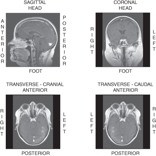Orthogonal slices are those in which only the ,, or gradient is used as the slice selection gradient. Oblique slices, those not in one of the principal directions, are obtained by applying more than one physical gradient when the RF pulse is broadcast. The total gradient amplitude, whether from one, two, or three physical gradients, determines the slice thickness as shown in equation (4.3). When images are viewed on the monitor or film, the slice selection direction is always perpendicular to the surface; that is, hidden from the viewer (Figure 4.4).

Figure 4.4 Images in standard slice orientations: sagittal, coronal, and transverse or axial. For transverse images, two view directions are possible: cranial and caudal. Image annotations are based on patient axes.

4.3 Readout or frequency encoding

---

The signal detection portion of the MRI measurement is known as Readout or Frequency Encoding. The readout process differentiates MRI from MR spectroscopy, the other type of MR experiment (see Chapter 13). In an imaging pulse sequence, the MR signal is always detected in the presence of a gradient known as the readout gradient , which produces one of the spatial dimensions of the image. A typical pulse sequence uses some form of excitation, such as a 90° slice-selective pulse, to excite a particular region of tissue. Following excitation, the net magnetization within the slice is oriented transverse to and will precess with frequency processes induce dephasing of this transverse magnetization (see Chapter 3). This dephasing can be partially reversed to form an echo by the application of a 180° RF pulse, a gradient pulse, or both. As the echo is forming, the readout gradient is applied perpendicular to the slice direction. Under the influence of this new gradient field, the protons precess at different frequencies depending on their position within it, in accordance with equation (4.2). Each of these frequencies is superimposed into the echo. At the desired time, the echo signal is measured by the receiver coil and digitized for later Fourier transformation. The magnitude of the readout gradient and the frequency that is detected enable the corresponding position of the proton to be determined (Figure 4.5).

Figure 4.5 Readout process. Following excitation, each spin within the excited volume (slice) precesses at the same frequency. During detection of the echo, a gradient is applied, causing a variation in the frequencies for the spins generating the echo signal. The frequency of precession for each spin depends on its position according to equation (4.2). Frequencies measured from the echo are mapped to the corresponding position.

The magnitude of is determined by two user-definable parameters: the field of view (FOV) in the readout direction, , and the Nyquist frequency for the image, often referred to as the receiver bandwidth (equation (2.2)). This relationship is expressed in the following equation:

4.4

where is the total range of frequencies in the image. is chosen so that protons located at the edge of precess at the Nyquist frequency above the transmitter frequency for the image (Figure 4.6). Smaller values can be achieved by increasing , keeping the Nyquist frequency and thus the total frequency bandwidth constant (Figure 4.7).

Figure 4.6 In any image, one of the directions visualized is the readout direction and the other is the phase-encoding direction. A proton located at the edge of the FOV in the readout direction precesses at the Nyquist frequency above or below the transmitter frequency . Changing the FOV of the image changes the spatial resolution (millimeters per pixel) but not the frequency resolution (hertz per pixel).

Figure 4.7 For a given range (bandwidth) of frequencies that are measured in the signal, the desired FOV is determined by the readout gradient amplitude. The user interface typically allows variation of the FOV, which is achieved by increasing or decreasing the readout gradient amplitude, as appropriate.

---

In an MR image, the resolution may be expressed in one of two ways: the spatial resolution and the frequency resolution. The spatial resolution, expressed as the voxel size with units of mm/pixel, is derived from two user parameters, and the number of readout sample points in the acquisition matrix, :

4.5

The frequency resolution, with units of Hz/pixel, is based on and for the image:

4.6

It is possible to improve the frequency resolution for the measurement independent of the spatial resolution by increasing the total sampling time used to measure the signal. This reduces the Nyquist frequency for the image and the background noise contributing to the measurement. In order to maintain the correct spatial resolution within the image, is reduced, in accordance with equation 4.4.

4.4 Phase encoding

The third direction in an MR image is the phase encoding direction. It is visualized along with the readout direction in a two-dimensional (2D) image (see Figure 4.5). The phase encoding gradient, , is perpendicular to both and and is the only gradient that changes amplitude during the data acquisition loop of a standard 2D imaging sequence. Any signal variation detected from one acquisition to the next is assumed to be caused by the influence of during the measurement.

---

The principle of phase encoding is based on the fact that the proton precession is periodic in nature. Prior to the application of , a proton within a slice precesses at the base frequency . In the presence of , its precessional frequency increases or decreases along the PE direction according to equation (4.2). Once is turned off, the proton precession returns to its original frequency, but is ahead or behind in phase relative to its previous state. This phase difference alters the amplitude that the proton will contribute to the final signal. The amount of induced phase change depends on the magnitude and duration of that the proton experienced and the proton location. Protons located at different positions in the phase encoding direction experience different amounts of phase shift for the same pulse (Figure 4.8). A proton located at the edge of the chosen FOV experiences the maximum amount of phase change from each phase encoding step. The MR image information is obtained by repeating the slice excitation and signal detection multiple times, each with a different amplitude of .

Figure 4.8 Concept of phase encoding. Prior to application of , all spins precess at the same frequency. When is applied, a spin increases or decreases its precessional frequency, depending on its position . A spin located at experiences no effect from and no change in frequency or phase . A spin located at precesses faster while is applied. Once is turned off, the spin precesses at its original frequency but is ahead of the reference frequency (dashed curve); that is, a phase shift has been induced to the proton by . A spin located at decreases its frequency while is applied. Once is turned off, it precesses at its original frequency but is behind the reference by a phase shift of .

The spatial resolution in the phase encoding direction depends on two user-selectable parameters, the field of view in the phase encoding direction, , and the number of phase encoding steps in the acquisition matrix, . The is determined by the change in from one step to the next. For a proton located at the chosen , each phase encoding step induces one half-cycle (180°) of phase change relative to the previous phase encoding step, assuming a constant pulse duration (Figure 4.9). determines the total number of cycles of phase change produced at the edge of the FOV and thus the maximum frequency in the phase encoding direction for the given pulse duration. The spatial resolution in the phase encoding direction is expressed as the voxel size and is measured in mm/pixel:

4.7

Increased resolution is obtained by reducing the or by increasing . The FOV reduction is accomplished by increasing the gradient amplitude change from one to the next.

Figure 4.9 Phase-encoding process. A spin at the edge of the FOV in the phase-encoding direction undergoes 90° of phase change from one phase-encoding step to the next. Each point within the FOV undergoes progressively less phase change for the same gradient amplitude. A spin at isocenter never experiences any phase change. The change in gradient amplitude ( in this example) from one phase-encoding step to the next is inversely proportional to the FOV .

---

Because of the two different physical processes involved, is not required to be the same as the , nor is the voxel size. The resulting pixel dimensions also need not be equal. The readout pixel size divided by the phase encoding pixel size is known as the aspect ratio between the two dimensions. An aspect ratio of 1.0 (100%) means that the pixel size is the same in both directions, a situation referred to as isotropic pixels. An aspect ratio less than 1.0 (<100%) is referred to as anisotropic pixels, with the phase encoding dimension typically larger than the readout dimension.

4.5 Sequence looping

The previous two sections described the individual steps used for spatial localization of the MR signal to a point within a slice. For most MR applications, information from many slices is measured during the scan in order to acquire images from large volumes of tissue. Several approaches are used for data acquisition that balance the desire for good spatial resolution and contrast-to-noise ratio (signal difference relative to background noise) while maintaining reasonable scan times.

In order to accomplish efficient data collection with minimal computer processing, most MRI techniques use some form of repetitive execution, which is achieved using computer instructions known as loops. This allows common instructions such as fixed amplitude gradient pulses (e.g., readout or slice selection gradient pulses) to be programmed one time yet provide a convenient method for modifying variable quantities such as phase encoding gradient amplitudes or RF pulse center frequencies.

There are several ways to differentiate measurement techniques. One method is based on the volume of tissue excited that is used to generate the signal. The most common technique is 2D multislice imaging, in which a narrow volume of tissue (typically ) is excited by a slice-selective RF pulse and generates the echo signal. The TR specified by the user is the time between successive excitation pulses for a given slice. The total number of lines of data collected for each slice depends on the number of phase encoding steps, , and the number of signals added together for signal averaging, . The sequence kernel time, or minimum TR per slice, is the actual time required for the measurement hardware to perform all the steps necessary to acquire raw data from a single excitation, typically one line from one slice. Often, the sequence kernel time is much shorter than TR, allowing excitation and detection of many slices to be performed within one TR time period.

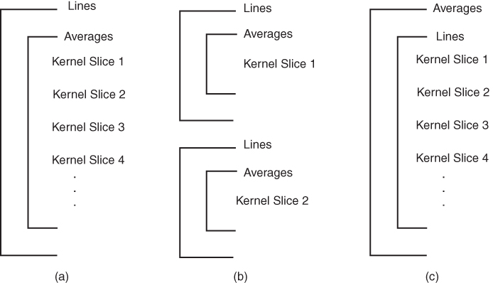
Traditionally, multislice scanning acquired one line of data from each slice during each TR time period (Figure 4.10a). This approach set a lower limit for TR. By subdividing the slice loop into subloops so that a subset of slices is acquired, a shorter TR and greater contrast control is possible. The total scan time is TR times the total number of lines times the number of subloops:

4.8

Two multislice loop structures are commonly used. Traditional multislice looping uses (Figure 4.10a), so that one line of data is acquired for each slice prior to measurement of a second line of data from any slice. The maximum number of slices is limited by TR. This provides the most efficient data collection process for a given TR and is useful when TR is relatively long. At the midpoint of a scan using this looping scheme, each image has lines of raw data, each with the requested number of acquisitions.

Figure 4.10 Two-dimensional slice loop structures. Three slice loop structures are commonly used. (a) Traditional multislice looping. The slice loop is the innermost loop ( not indicated). Each slice is excited and signal-detected prior to any slice being excited a second time for purposes of signal averaging or phase encoding (lines). This loop structure is the most common. (b) Sequential slice looping. All information for a given slice is acquired prior to any excitation for a different slice. In this figure, . (c) Long-term averaging. All lines for all slices are acquired before performing signal averaging.

The other approach uses equal to the number of slices (Figure 4.10b), a so-called sequential slice technique. In this technique, all information for a slice is acquired before acquiring any information for another slice. Only one line of data is measured during each TR time period. This allows the use of very short TR times when acquiring large numbers of slices. At the midpoint of a scan using this looping scheme, all the data for one-half the requested number of slices has been acquired.

There is also variability in the order of the main loops for 2D multislice imaging. Traditional looping as in Figure 4.10a acquires all signals for a specified phase encoding step (all slices, all averages) before acquiring a signal for a different phase encoding step. This allows all signal averaging for a given raw data line to be done within a short period of time and allows initial steps of image reconstruction to be performed. The other variation acquires a complete raw data set for a slice before beginning any signal averaging (Figure 4.10c). This increases the elapsed time between successive signals being averaged together, reducing any possible contamination between the signals, but renders the image more susceptible to gross patient motion.

The other category of measurement technique is a 3D volume acquisition, which is, in essence, a double phase encoding technique. For 3D volume imaging, tissue volumes of 30–150 mm are excited as compared to 3–10 mm in 2D imaging. In addition, a second phase encoding table is applied in the slice selection direction to “partition” or subdivide the volume into individual slices. Each echo is acquired following application of encoding gradients in both the phase encoding and slice selection directions, one amplitude from each.

The advantages of 3D volume acquisition techniques are that the slices within a volume are contiguous and that the detected signal is based on the total volume of excitation rather than the effective slice thickness. The 3D volume acquisitions have two primary disadvantages. Because of the potentially long scan times, they are usually gradient echo or echo train spin echo sequences and are limited to one or two volumes. Image processing is also longer since an additional Fourier transformation and other processing steps must be performed in order to produce an image.

For 3D volume MRI techniques, in each excitation volume the number of slices is determined by the number of partitions, . The total scan time is:

4.9

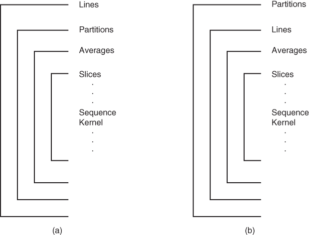
There are two possibilities for the order of the two encoding loops. Traditional looping has the partitions loop inside the phase encoding loop (Figure 4.10a), typical of 3D gradient echo techniques. Since the partitions loop normally has fewer entries, this enables initial image processing to be performed while data collection continues. The other order has the phase encoding loop inside the partitions loop (Figure 4.11b). This is more typical for 3D echo train spin echo, where the phase encoding loop is segmented in nature (see Chapter 5).

Figure 4.11 Three-dimensional slice loop structures. A fourth loop, the partitions loop, is added. Two slice loop structures are commonly used: (a) partitions-in-lines: the partitions gradient amplitudes are varied most frequently; (b) lines-in-partitions: the lines gradient amplitudes are varied most frequently.