Chapter 10
Motion artifact reduction techniques

As discussed in Chapter 9, motion in an MR image can produce severe image artifacts in the phase encoding direction. The severity of the artifact depends on the nature of the motion, the time during data collection when the motion occurs, and the particular pulse sequence and measurement parameters. The most critical portion of the data collection period for artifact generation is during the measurement of echoes following low-amplitude phase encoding steps (center of -space). Motion during the high-amplitude phase encoding steps (edges of -space) can cause blurring but not severe signal misregistration in the image.

Four methods are commonly used to reduce the severity of the motion artifact on the final image. If signal from the moving tissue is not of interest, use of a spatial presaturation pulse as described in Chapter 8 can significantly reduce artifactual signal. This is useful to suppress abdominal or cardiac motion artifacts in spine examinations. The other techniques are useful when signal from the moving tissue is desired. Two of these, acquisition parameter modification and physiological triggering, affect the mechanics of the data collection process, while the third method, flow compensation, alters the intrinsic signal from the moving tissue. Although none of these approaches completely removes motion artifacts from the image, use of one or more of these techniques substantially reduces the impact of motion on the final images.

10.1 Acquisition parameter modification

Proper choice of the acquisition parameters can alter the appearance of motion artifacts. One example of this is to define the phase encoding direction so that the motion artifact does not obscure the area of interest. This may be referred to as motion artifact rotation or swapping the frequency and phase encoding directions as the physical gradient directions for PE and RO are switched. This approach does not eliminate or minimize the artifact, but only changes its position within the image. For example, motion artifacts due to eye movement or blood flow from the sagittal sinus vein may obscure lesions in the cerebrum if the phase encoding direction for a transverse slice is in the anterior–posterior direction. If the phase encoding direction is in the left–right direction, the eye motion artifacts lie outside the brain. The blood flow artifact also appears in an area outside the brain (Figure 10.1).

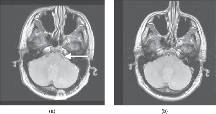
Figure 10.1 The direction of motion artifacts is determined by the phase-encoding gradient. Blood flow during the scan produces motion artifact (arrow). (a) RO: left/right, PE: anterior/ posterior; (b) RO: anterior/posterior, PE: left/right.

Another example of parameter modification is to increase the number of signal averages. This approach is of particular benefit in abdominal imaging where respiratory motion can produce severe ghosting. With multiple averages, the signal from the tissue is based on its average position throughout the scan. Since the tissue is in the same location most of the time, the signals add coherently. The motion artifact signal will be reduced in amplitude relative to the tissue signal.

Alternately, removal of respiratory artifacts in abdominal or cardiac imaging can be accomplished by measuring all the scan data within one breath-hold. For example, a , and can produce a complete scan in 18 seconds. The spatial resolution may be compromised in the phase encoding direction, depending on the , but respiratory motion and its artifacts will not be present if the patient suspends respiration. Extreme examples of this approach are single-shot echo train spin echo and EPI techniques, where images can be acquired in less than one second, producing heart and bowel images that are virtually motion–artifact free (Figure 10.2).

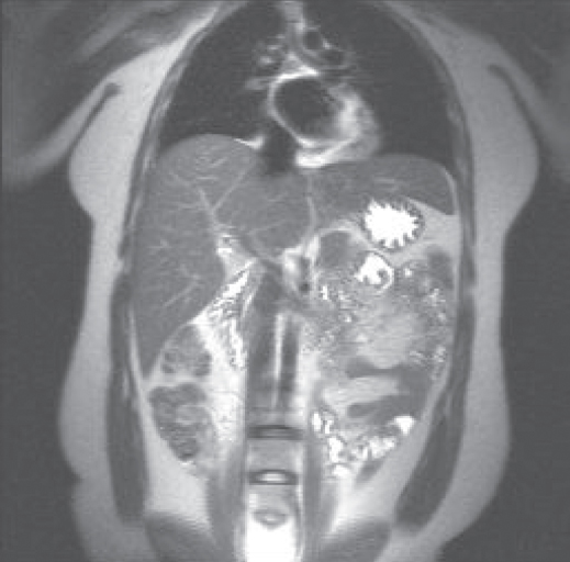
Figure 10.2 Single-shot echo train spin echo image of abdomen. Note lack of motion artifact from heart and bowel.

10.2 Triggering/Gating

Another method for visualizing moving tissue allows the tissue to move but synchronizes the data collection with a periodic signal produced by the patient, such as a pulse or heartbeat. The data collection–timing signal relationship can be exploited in two ways. Prospective methods initiate the data collection following detection of the timing signal. The signal detection for a particular slice always occurs at the same time following the timing signal. Since the moving tissue is in the same relative position at this time, there is minimal misregistration of the signal and a significant reduction of the resulting motion artifact. Retrospective methods measure the timing signal together with the echo signal, but the timing signal is not analyzed nor the measured data adjusted until the scan is completed. The data collection process can also be triggered by or gated to the timing signal.

Triggering examinations are commonly prospective in nature and begin the data collection following detection of a signal. The noise produced by the scanner during sequence execution is also synchronized to the signal source. The TR controlling the contrast is based on the repetition time for the trigger signal rather than the TR entered in the user interface. Several external methods for detection of the timing signal can be used. For cardiac imaging, data collection is synchronized to the electrocardiogram (ECG) signal measured from the patient using lead wires. Pulse triggering uses a pulse sensor to detect the pulse, usually measured on an extremity. Respiratory triggering uses a pressure or strain transducer attached to the patient to measure either chest or abdominal motion. An internal method for a timing reference uses a so-called “navigator echo” that, when properly positioned, can measure an MR signal from the diaphragm or other tissue and indicate that motion has occurred.

There are several potential problems with triggered studies. One is that the scan time is longer for a triggered study than for the corresponding untriggered study. Time must be allowed from the end of data collection (traditionally TR) to the next trigger signal to ensure that the trigger signal is properly detected by the measurement hardware. This extra time is usually 150–200 ms to allow for variation of the rate of the trigger signal for the patient. The total scan time will be extended by approximately 1–2 minutes. Another problem occurs if the rate of the trigger signal is irregular. The for a particular phase encoding step depends on the R–R time interval immediately prior to the step under consideration. Variation in the heart rate causes variation in the amount of T1 relaxation from measurement to measurement for each phase encoding step. This variation produces amplitude changes in the detected signal, producing misregistration artifacts in the final images even if the triggering is perfect. Stability of the heart rate is most critical during collection of the echoes around the -space center .

Cardiac examinations are one example of an examination that typically uses prospective triggering. The peak R wave is normally used as the timing reference point. Each phase encoding step is acquired at the same point in time following the R wave so that the heart is in the same relative position (Figure 10.3). Since the kernel time per slice is shorter than the duration of the R–R interval , several signals can be acquired within one heartbeat. Proper detection of the ECG signal from the patient is critical. Improper electrode placement may detect significant signal from the blood during its flow through the aortic arch. In addition, the transmitted RF energy and the gradient pulses may also interact with the lead wires, inducing significant noise to the detected ECG signal. High-resistance lead wires may even burn the patient through this coupling.

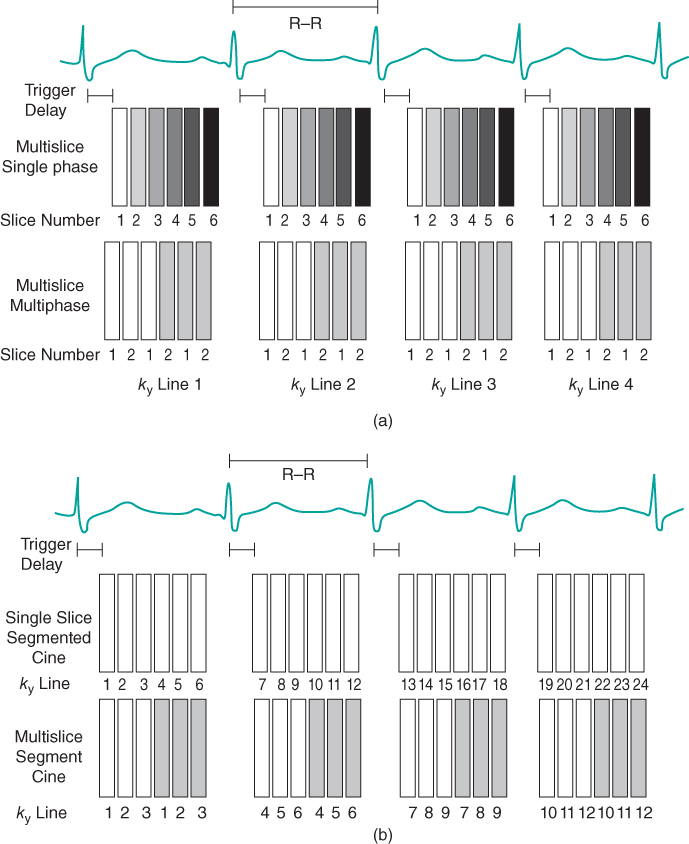
Figure 10.3 Triggered data collection. The R wave is used as a timing signal. A trigger delay (TD) can be used to initiate data collection at any time desired during the cardiac cycle. (a) Nonsegmented measurement. For multislice single-phase imaging, one line for each slice is acquired per heartbeat. Information for a particular slice is acquired at the same time following the R wave. The T1 contrast is based on the R–R time interval rather than the user-defined TR. Alternatively, a multislice, multiphase acquisition may be carried out in which slices are acquired at different times during the cardiac cycle at the same position. (b) Segmented measurement. For single-slice imaging, multiple lines are acquired for a particular slice following the R wave. For multislice imaging, multiple lines are acquired for multiple slices following the R wave.

Historically, triggered examinations used spin echo sequences for data collection, in which one signal (line of -space) was acquired per slice per heartbeat. Each image within the scan is acquired at a different position and a different time point in the cardiac cycle. These images were typically T1-weighted (depending on the R–R time interval) with a minimal blood signal and were used for morphological studies of the heart. Current scan techniques use gradient echo sequences in a segmented manner to acquire multiple lines of -space per slice per heartbeat. This allows a complete raw data set to be acquired in fewer heartbeats, which reduces the scan sensitivity to a variable heart rate. In many cases, the scan times are short enough for patients to suspend respiration, which reduces artifacts from respiratory motion. These scans may use a spoiled gradient echo sequence to produce morphologic images (Figure 10.4), or a partially or totally refocused gradient echo sequence to produce images with a bright blood signal. Rapid display of these images allows a dynamic or cine visualization of the heart and cardiac hemodynamics during the different phases of the cardiac cycle (Figure 10.5). Prospective cine examinations have a problem that the initial image in the data set, representing the first phase of the cardiac cycle for the scan, will often be brighter than the subsequent images in the scan. This is due to the longer amount of T1 relaxation that the net magnetization undergoes for this time point compared to the other images, due to the “dead” time waiting for the trigger pulse.

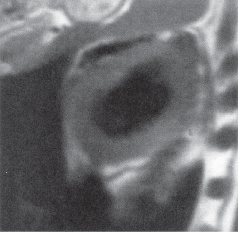
Figure 10.4 Short-axis T1-weighted image acquired using a triggered multislice mode.

Figure 10.5 Cine heart images acquired at different phases of cardiac cycle. Measurement parameters: pulse sequence, two-dimensional spoiled gradient echo; TR, 35.4 ms; TE, 1.5 ms; excitation angle, 65°; acquisition matrix, , 108 and , 128; FOV, 169 mm PE × 200 mm RO; , 1. (a) 92 ms following R wave; (b) 552 ms following R wave.

Gating methods typically have the sequence continuously executing RF and gradient pulses but not measuring signal, and link the timing signal to the time when echoes are actually measured. The continuous execution maintains a relatively constant net magnetization so that all images will have comparable contrast. Prospective gating has been used in cardiac imaging and in abdominal imaging to reduce artifacts from respiratory motion. Two approaches are used, both of which synchronize the data collection to the respiratory cycle of the patient. Simple respiratory gating acquires the data when there is minimal motion. It suffers from significantly longer scan times since the time during respiratory motion is not used for data collection. An alternative technique used for T1-weighted imaging, respiratory compensation, rearranges the order of phase encoding so that adjacent G_PE are acquired when the abdomen is in the same relative position. Typically, the low-amplitude are acquired at or near end expiration so that the echoes contributing the most signals are measured when there is the least motion. Higher amplitude are acquired during inspiration. Significant improvement of respiratory-induced ghosts can be achieved by either technique as long as there is a uniform respiration rate during the scan. Nonuniform respiration may produce artifacts as severe as those produced from a nongated scan.

An alternative to prospective triggering for cine heart imaging is known as retrospective gating. In this approach, the ECG signal is measured but the data collection is not controlled by the timing signal. Instead, the data are measured in an untriggered fashion and the time following the R wave when each phase encoding step was measured is stored with it. Following completion of the data collection, images are reconstructed corresponding to various time points within the cardiac cycle. The data for any phase encoding step not directly measured are interpolated from the measured values.

10.3 Flow compensation

Another method for reducing motion artifacts adds additional gradient pulses to the pulse sequence to correct for phase shifts experienced by the moving protons. It is known as flow compensation, gradient motion rephasing (GMR), or the motion artifact suppression technique (MAST). As described in Chapter 6, gradient pulses of equal area but opposite polarity are used to generate a gradient echo. Proper dephasing and rephasing of the protons and correct frequency and phase mapping occur as long as there is no motion during the gradient pulses. Movement during either gradient pulse results in incomplete phase cancellation or a net phase accumulation at the end of the second gradient pulse time. The amount of phase accumulation is a function of the velocity of the motion. This residual phase accumulation produces signal intensity variations that are manifest as motion artifacts in the phase encoding direction (Figure 10.6a), regardless of the direction of the motion or the gradient pulses.

Figure 10.6 Flow compensation. Use of flow compensation gradient pulses will map moving protons such as cerebrospinal fluid to their proper location. Measurement parameters are: pulse sequence, spin echo; TR, 2500 ms; TE, 90 ms; excitation angle, 90°; acquisition matrix, , 192 and , 256 with twofold readout oversampling; FOV, ; , 1; slice thickness, 5 mm. (a) No flow compensation. Misregistration artifact from CSF flow appears anterior to the spinal canal (arrow). (b) First-order flow compensation in readout and slice-selection directions. CSF is properly mapped into the spinal canal.

If the velocity of the protons is approximately constant during the gradient pulse then the motion-induced phase changes can be corrected by applying additional gradient pulses. These pulses will be applied in the direction for which compensation is desired. The duration, amplitude, and timing of the pulses can be defined so that protons moving with constant velocity can be properly mapped within the image, and similar methods exist for acceleration, etc. (Pipe and Chenevert, 1991). For gradient echo sequences, velocity compensation is normally sufficient for proper registration of cerebrospinal fluid, while for spin echo sequences, higher order compensation can often be achieved with minimal complications (Figure 10.6b).

Flow compensation requires that certain limitations be placed on the pulse sequence. Since additional gradient pulses are applied during the slice loop, the minimum TE for the sequence must be extended to allow time for their application. In pulse sequences where short TEs are desired, higher amplitude gradient pulses of shorter duration may be used. This will limit the minimum FOV available for the sequence. In practice, only modest increases in TE and the minimum FOV are normally required.

10.4 Radial-based motion compensation

A final method for motion compensation is based on the fact that radial scanning always acquires data through the center of -space. These lines can be used to correct for in-plane motion in the image, as the points near the center should have a comparable signal regardless of the gradient direction. One method of data collection uses a segmented data collection as in echo train spin echo, except that each echo train acquires lines of data near the center of -space at different angles (view directions) (Figure 10.7). This method, known as PROPELLER or BLADE, creates an image of low spatial resolution to correct for motion. It requires a regridding of the data to ensure that there are no gaps in the raw data, but can produce images with good image quality with minimal motion artifact.

Figure 10.7 Radial motion compensation. Each scan measures a portion of k-space (dark lines). Some of the measured lines contain points acquired at the center of k-space.