Chapter 6
Pulse sequences
A pulse sequence is the measurement technique by which an MR image is obtained. It contains the hardware instructions (RF pulses, gradient pulses, and timings) necessary to acquire the data in the desired manner. As implemented by most manufacturers, the pulse sequence actually executed during the measurement is defined from parameters directly selected by the operator (e.g., TR, FOV) and variables defined in template files (e.g., basic relationships between RF pulses and slice selection gradients). This allows the operator to create a large number of pulse sequences using a limited number of template files. It also enables the manufacturer to limit parameter combinations to those suitable for execution. Some parameter limits of a pulse sequence (e.g., minimum TR, minimum FOV) depend on how the manufacturer has implemented the technique (e.g., gradient pulse duration), while other parameters (e.g., maximum gradient amplitude, gradient rise time) are determined by performance limits of the scanner hardware. The effect of common operator-selectable parameters on the signal intensity produced from a volume element of tissue is discussed in more detail in Chapter 7.
One of the more confusing aspects of MRI is the wide variety of pulse sequences available from the different equipment manufacturers and the even wider variety of pulse sequence names. In addition, similar sequences may be known by a variety of names by the same manufacturer. As a result, comparison of techniques and protocols between manufacturers is often difficult due to differences in sequence implementation. An accurate description and detailed comparison of techniques between manufacturers would require knowledge of proprietary information. Fortunately, there is an effort underway to provide a standardization of sequence nomenclature (DIN, 2008). This chapter describes several pulse sequences commonly used in imaging by all manufacturers and some of the general characteristics of each one. In addition, where appropriate, the common acronyms used by some of the major manufacturers for the sequences are included.
Comparison of pulse sequences is facilitated by the use of timing diagrams. Timing diagrams are schematic representations of the basic steps performed by the different hardware components during sequence execution. Although there may be stylistic differences in the diagrams prepared by different authors, the general features are the same for all diagrams (Figure 6.1). Elapsed time during sequence execution is indicated from left to right along the horizontal axis. The vertical separation between lines is employed only for visualization. Each horizontal line corresponds to a different hardware component. At a minimum, four lines are used to describe any pulse sequence: one representing the radiofrequency (RF) transmitter and one representing each gradient (labeled as  ,
,  , and
, and  , or
, or  ,
,  , and
, and  ). Additional lines may be added to indicate other activity such as analog-to-digital converter (ADC) sampling. Activity for a particular component such as a gradient pulse is shown as a deviation above or below the horizontal line (baseline). Simultaneous activity from more than one component such as the RF transmitter and slice selection gradient is indicated by nonzero activity from both lines at the same horizontal position. Constant-amplitude gradient pulses are shown as simple deviations from the baseline. Gradient tables such as for phase encoding are represented as hashed regions or sections with horizontal lines. Timing diagrams typically represent the hardware activity for the fundamental repeating unit of the pulse sequence, often called the kernel of the sequence. Specific details regarding exact timings, individual gradient amplitudes, or looping structures are not included as much of this information is determined by the specific measurement parameters or is proprietary to the various manufacturers. The generic nature of the representations makes timing diagrams suitable to represent classes of pulse sequences when making comparisons between the various measurement techniques.
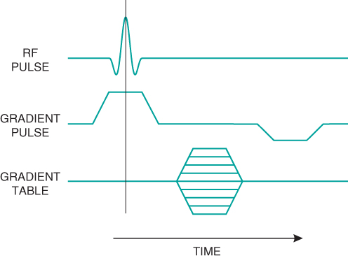
Figure 6.1 Simple timing diagram. The horizontal axis is time during sequence execution. Control signals for three hardware components are illustrated: the RF transmitter and two gradients (labeled RF Pulse, Gradient Pulse, and Gradient Table). The gradient pulse signals are executed the same way for each measurement, as indicated by the trapezoidal shape for the two gradient pulse waveforms. The gradient table signals change amplitude with each measurement and are represented by the multiple horizontal lines.
6.1 Spin echo sequences
Standard multiecho sequences apply multiple 180° refocusing RF pulses following a single excitation pulse. Each refocusing pulse produces a spin echo, each one at a different TE defined by the user. A single  is used per RF excitation pulse (Figure 6.3). Differences in raw data signal intensity at each TE are still due to differences in
  only. This approach introduces raw data signal intensity variations from echo to echo (
 to
to  ) due to T2 relaxation. Images are created from the signals acquired at a single TE time. Multiecho sequences are used to produce proton density-weighted images using short TE (less than 30 ms) and T2-weighted images using long TE (greater than 80 ms) when TR is long enough to allow relatively complete T1 relaxation for most tissues (2000 ms or longer).
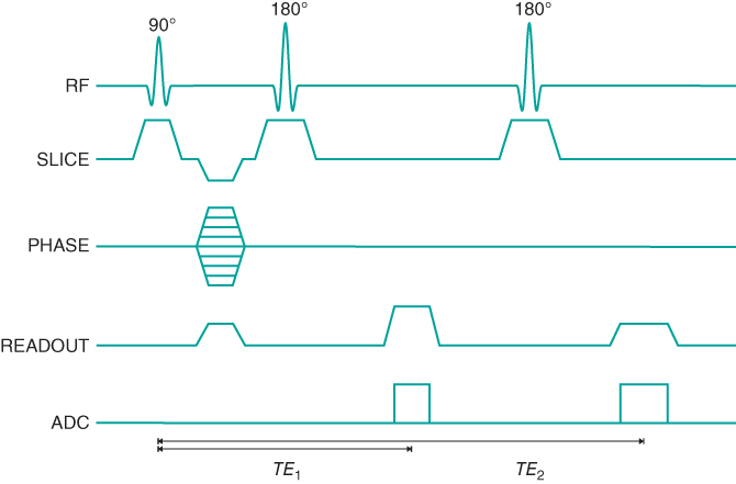
Figure 6.3 Standard multiecho spin echo sequence timing diagram. Two echoes are illustrated. Additional echoes may be generated by adding additional 180° RF pulses, slice-selection gradient pulses, readout gradient pulses, and ADC sampling period. Note the single phase-encoding gradient table. Both TE times are measured from the middle of the excitation pulse to the center of the respective echo.
The contrast in ETSE sequences is determined primarily by the echoes detected at or near  and the TEs for these echoes. The TE assigned to the image is referred to as an effective TE since there are echoes with different TEs contributing to the final image. This use of multiple TEs in the creation of the image makes ETSE sequences unsuitable for use when subtle differences in T2 between tissues are responsible for the image contrast. Fat will also have an increased signal compared to standard spin echo or multiecho images acquired with the same TE.
While ETSE sequences can be used to produce T1-weighted images, their most common application has been to produce T2-weighted images. This is due to the significant reduction in scan time that can be achieved for long TR scans when modest echo train lengths are used. While echo train lengths less than 10 are typically used for brain and spine imaging, very long echo trains (100 or more) can be used in abdominal imaging to acquire T2-weighted images in less than one second. Termed snapshot or ultrafast ETSE, the scan times are sufficiently short to freeze bowel motion, yet provide good T2 contrast between tissues.
6.2 Gradient echo sequences
The simplest gradient echo sequence is a spoiled gradient echo sequence. This sequence uses a spoiling scheme to dephase the transverse magnetization following signal detection. As a result, only longitudinal magnetization contributes to  at the time of the next excitation pulse. Spoiling may be done either by applying high amplitude gradient pulses known as “spoiler” or “crusher” gradients to dephase the magnetization or by varying the phase of the RF excitation pulse in a pseudorandom fashion following each application. This approach, known as RF spoiling, produces an incoherent addition of any residual transverse magnetization so that the only remaining coherence at the time of the next excitation pulse is in the longitudinal direction (Figure 6.5).
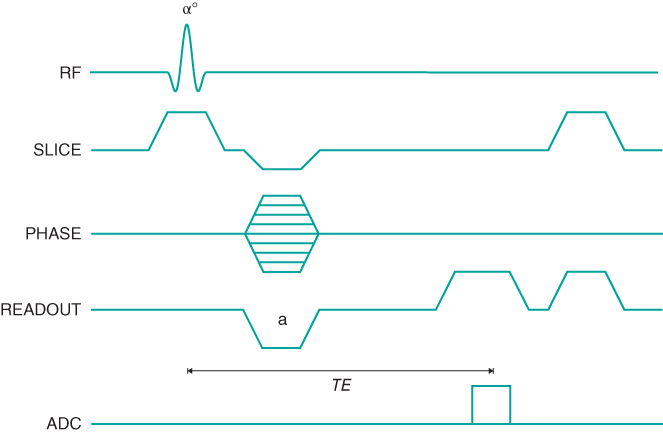
Figure 6.5 Spoiled gradient echo sequence timing diagram, two-dimensional method. Because there is no 180° RF pulse, the polarity of the  dephasing gradient pulse (a) is opposite that of the readout gradient pulse applied during signal detection. Gradient spoiling is illustrated at the end of the kernel. The TE time is measured from the middle of the excitation pulse to the center of the echo.
In many respects, spoiled gradient echo sequences are the gradient echo counterpart of spin echo sequences. However, the contrast behavior of spoiled gradient echo techniques is slightly more complicated. The TE determines the amount of T2* rather than T2 weighting. The combination of excitation angle and TR determines the amount of T1 weighting. Low excitation angle pulses impart minimal RF energy and leave most of  in the longitudinal direction. This allows a shorter TR to be used without producing saturation of the protons. Proton density-weighted images are produced for small excitation angles (15–20°), relatively long TR (500 ms), and short TE
  . T2* weighted images can be obtained using the same excitation angle and TR but a long TE (25–30 ms). Substantial T1 weighting is obtained using large excitation angles (80° or greater), short TR (100–150 ms), and short TE
  .
.
Spoiled gradient echo images may be acquired using any of the sequence looping techniques discussed in Chapter 4. Routine spoiled gradient echo imaging for spinal or abdominal studies uses a 2D multislice mode. A 2D sequential mode is used for MR angiography (see Chapter 11) while a 3D volume acquisition can produce very thin slices useful for multiplanar reconstruction of images in arbitrary orientations.
A second group of gradient sequences belongs to a class of techniques known as refocused or steady-state gradient echo sequences. Refocused gradient echo sequences use a single excitation pulse with a TR shorter than the T2 relaxation time and do not use spoiling. Once  has reached a steady-state value (following a few RF pulses), both longitudinal and transverse components are present at the time of the next excitation pulse. Unlike spoiled gradient echo sequences, refocused sequences apply rephasing gradient pulses in one, two, or all three directions to maintain the transverse magnetization as much as possible. In addition, the excitation pulses are applied rapidly enough (short TR) so that spin echoes are generated that occur simultaneously with the subsequent excitation pulses. These spin echoes refocus the transverse magnetization as in spin echo imaging so that the signal amplitude in refocused pulse sequences depends strongly upon the T1 and T2 relaxation times of the tissues under observation. Optimal contrast can only be achieved in tissues with long T1 and T2 relaxation times.
Two signals can be measured from a refocused pulse scheme, one before and one after the refocusing pulse (Figure 6.6). This scenario is analogous to examining a normal spin echo and using the protons as they rephase prior to TE to produce one signal and as they dephase following TE to produce the other signal. In spin echo imaging, both halves of the echo are detected and are processed together. In gradient echo imaging, each half of the echo can produce an image. The two pulse sequences are complementary in their sequence timing (Figure 6.7). The technique using the postexcitation pulse signal is conceptually similar to the spoiled gradient echo technique except for the unspoiled transverse magnetization.
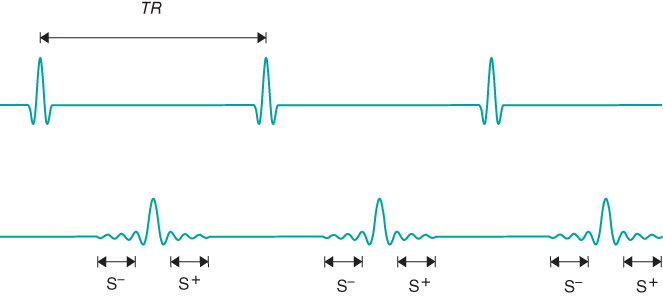
Figure 6.6 A series of equally spaced RF pulses produces spin echoes that form at the time of the subsequent RF excitation pulses. Once a steady state is reached (following several  time periods), signal is induced prior to and following the excitation pulse. The preexcitation pulse signal
  is strictly echo reformation. The postexcitation pulse signal
  is a combination of echo and free induction decay. Images can be produced from either signal or from both.
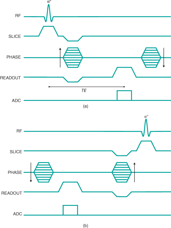
Figure 6.7 Refocused gradient echo sequence timing diagrams. Instead of spoiling the transverse magnetization, rephasing gradients are used to maintain the transverse magnetization as much as possible. (a) Postexcitation imaging sequence; (b) preexcitation imaging sequence.
Bright signals are produced by both pre- and postexcitation techniques for tissues such as cerebrospinal fluid and blood with relatively long T2 values and when TR is short so that the transverse coherence is maintained. A difference between the two techniques is observed when using a long TR or for tissues with T2 that is much shorter than T1. In general, the postexcitation  signal in Figure 6.6 is based on net magnetization derived from two sources present at the time of the RF excitation pulse: the transverse magnetization
  produced by previous excitation pulses, which generates a spin echo and decays based on T2 relaxation, and the longitudinal magnetization
  resulting from T1 relaxation, which generates an FID and decays based on T2*.
Elimination of this  component is accomplished in two ways. The use of spoiling, either gradient-based or RF-based, explicitly removes this component as in spin echo sequences. Use of a long TR (e.g., 500 ms) with a small excitation pulse angle (10–15°) allows this component to decay naturally. In both approaches, only the
  component is present, so that the decay of S+ is based on T2*. This means that equivalent contrast results are obtained for spoiled and refocused gradient echo techniques if a long TR and low excitation pulse angle are used. For the preexcitation technique, the signal is derived from the
  component only so that, with spoiling or using long TR, no image is produced.
For refocused gradient echo sequences using short TR and a large excitation pulse angle, the presence of the  component in
  increases the signal from tissue with long T2 such as fluid. The problem is that the two resulting transverse magnetizations can decay at different rates, particularly if the magnet homogeneity is not uniform. This causes a phase difference in those tissues to develop and can result in an interference banding artifact appearing in the postexcitation images if there is a significant signal from the
  component (Figure 6.8). The use of refocusing gradients retains this component as much as possible, but the extent of banding increases with increased refocusing. Use of complete gradient refocusing (so-called steady-state free precession sequences) should be preceded by adjustment of the magnet homogeneity. This will increase the T2* for the
  -based signal and will reduce the extent of banding.
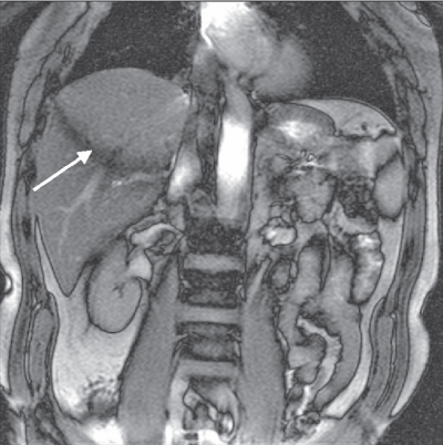
Figure 6.8 Coronal image acquired with fully refocused gradient echo technique. The arrow indicates a signal cancellation artifact due to interference between the pre-and postexcitation signals. (Reproduced with permission of H. Cecil Charles, Duke University.)
6.3 Echo planar imaging sequences
Two data collection schemes are used in EPI sequences: single-shot and segmented or multishot. Single-shot techniques acquire all phase encoding steps following a single excitation pulse. Since only one RF pulse is applied per slice position, each image can be acquired with an “infinite” TR. Modern gradient amplifiers may be required for single-shot EPI imaging because of the rapid switching of the readout gradient polarity necessary to acquire all the echoes. Segmented techniques acquire a subset of phase-encoding steps following each excitation pulse. A segmented loop structure with multiple excitation pulses is used to acquire all phase encoding steps. Segmented EPI can often be performed with older imaging gradient systems.
The contrast in EPI images is determined by the TE for the echo acquired when  . Each echo is acquired at a different TE similar to echo train spin echo sequences, so the TE of the image is referred to as an effective TE. Variations in contrast for EPI sequences are achieved using magnetization-preparation pulses (see Section 6.4) applied prior to the readout period. T1-weighted images are produced using a 180° inversion RF pulse prior to the excitation pulse. T2-weighted images can be obtained using a 90–180° pair of pulses to produce a spin echo. Spoiled gradient echo EPI sequences use no preparatory pulse and produce T2*-weighted images.
6.4 Magnetization-prepared sequences
The pulse sequences described previously provide the fundamental methods used for spatial localization in MRI today. For certain combinations of measurement parameters, the images that result from these techniques may have a lack of tissue contrast or poor spatial resolution. In order to overcome these limitations, the basic techniques may be modified using RF pulses to preset the net magnetization to a given state prior to execution of the spatial localization steps. These extra pulses are known as magnetization-preparation pulses and the sequences that incorporate them are collectively known as magnetization-prepared (MP) sequences.
The image reconstruction process will have a significant role in the appearance of IR-type images. The inversion of M by the 180° RF pulse allows for the generation of negative amplitude signals. Short TI times allow minimal T1 relaxation between the inversion and excitation RF pulses. Most tissues will have M inverted at the time of the excitation pulse. Long TI times allow more complete relaxation of tissues between the two pulses to occur, producing positive values for M. Intermediate TI gives a mixture of positive and negative M, depending on TI and the specific tissue T1 values (Figure 6.13). During image reconstruction, the phase of M can be incorporated into the pixel intensity. Termed phase-sensitive IR, these images have negative pixel values for tissues with inverted M. These are produced by tissues with long T1 values at short TI times. Background air is assigned a midrange pixel value. Phase-sensitive IR images have the largest range of pixel values of any imaging technique. Alternately, the phase of M can be ignored in the final image. Termed absolute value or magnitude IR, these images have pixel values based only on the signal magnitude. Tissues with very short or very long T1 relaxation times have high pixel values and background air has a low pixel value (Figure 6.14).
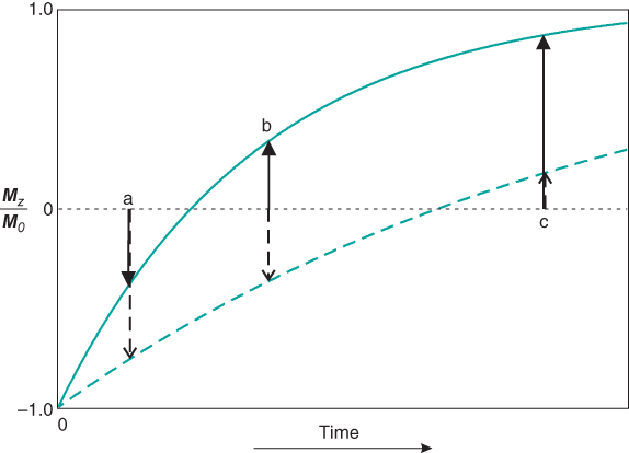
Figure 6.13 T1 recovery curves for inversion recovery sequences. The 180° inversion pulse inverts the net magnetization for all tissues. Tissue with a short T1 time (solid curve) recovers faster than tissue with a long T1 (dashed curve) time. For a TI time of (a), both tissues contribute significant negative amplitude signal. For a TI time of (b), the short T1 tissue contributes positive amplitude signal while the long T1 tissue contributes negative amplitude signal. For a TI time of (c), the short T1 tissue contributes significant positive amplitude signal and the long T1 tissue contributes minimal signal. If the signal polarity is considered (phase-sensitive IR sequences), signal difference will be seen at all three TI times. If the signal polarity is ignored (absolute value or magnitude IR sequences), no difference in signal between the two tissues will be seen at time (b).
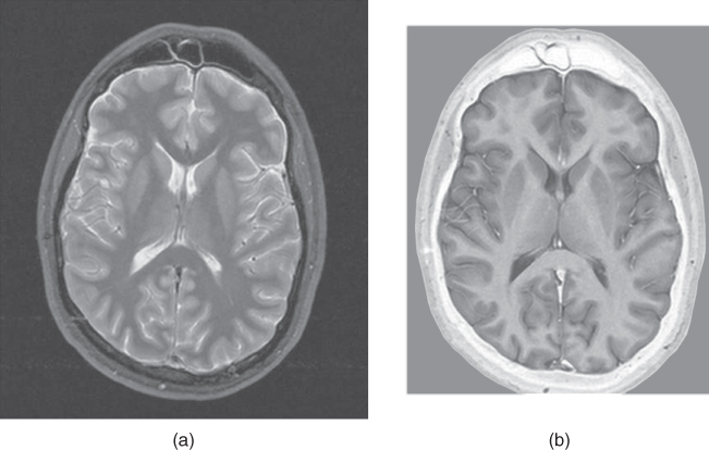
Figure 6.14 Magnitude (a) and phase-sensitive (b) inversion recovery images. All other measurement parameters are equal: pulse sequence, echo train spin echo, five echoes; TR, 7000 ms; TE, 14 ms; TI, 140 ms; acquisition matrix;  , 224 and
  , 256; FOV,
  RO;
RO;  , 1; slice thickness, 5 mm.
The inversion pulse also enables the suppression of signal through the proper choice of TI. If the TI time is chosen so that the tissue of interest has no longitudinal component at the time of the excitation pulse, then that tissue contributes no signal to the final image. This time, known as the null time for the tissue, is determined by the T1 relaxation time for the tissue:
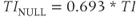
assuming that the TR time is sufficiently long. The two most common applications of IR sequences are for the suppression of cerebrospinal fluid (CSF) and fat. Normal CSF has a T1 relaxation time of approximately 3000 ms at 1.5 T. A TI time of 2080 ms applies the excitation pulse when the CSF magnetization has no longitudinal component and produces an image with no CSF signal. This technique, known as fluid-attenuated IR (FLAIR), allows easy visualization of gray and white matter inflammation.
Fat has a heterogeneous structure and its signal is a composite of all the tissue types within it. It has a T1 relaxation time of approximately 200–250 ms at 1.5 T. If a TI value of 140–160 ms is selected, the excitation pulse occurs when the fat magnetization has no longitudinal component and produces an image with no fat signal. This technique is known as STIR, or short TI inversion recovery. Virtually complete and uniform fat suppression throughout the imaging volume can be achieved using STIR imaging using the correct TI. However, it suffers from two major limitations. One is that the sequence kernel time is longer due to the TI time. As a result, a limited number of slices can be acquired for a typical TR. Complete coverage of the desired anatomical region may require the use of multiple scans or the ETSE sequence variation. The second problem occurs when using a T1 contrast agent. As described in Chapter 15, gadolinium-based contrast agents such as Gd-DTPA shorten the T1 relaxation time for the water in tissues that absorb the agent. Tissues with long T1 values that would normally be bright in a STIR image will lose signal if the contrast agent is present as the tissue T1 approaches that of the fat tissue. Visualization of these tissues thus becomes difficult. For this reason, STIR imaging is usually not performed when contrast agents are administered.
MP pulses can also be incorporated into gradient echo and EPI sequences. These pulses are often used to improve tissue contrast for scans where short measurement times are desired. For example, a TR of 7 ms with  will require 900 ms of scan time. The excitation angle must be between 5° and 10° to minimize saturation effects yet produce sufficient transverse magnetization to generate a signal. Added contrast may be obtained by manipulating the longitudinal magnetization through the application of additional RF pulses prior to the gradient echo sequence. These preparation pulses generate enhanced amplitude variations to M that can be measured during the rapid data collection time. This is the concept of MP gradient echo sequences. The same approach is used for single-shot EPI sequences. An inversion pulse is added prior to the excitation to provide T1 weight. The TI time is the primary parameter that controls the amount of T1 influence.
One major difference between the usage of MP pulses in gradient echo or EPI sequences compared to spin echo-based sequences is in the frequency of application of the MP pulse. Spin echo-based sequences apply one MP pulse per excitation pulse so that the MP-modified net magnetization has a steady-state value for the scan. In other words, the modified M will be constant at the time of the excitation pulse, though different from its value in the absence of the MP pulse. EPI sequences also apply one MP pulse per excitation pulse, but they are non-steady-state techniques since M does not have the same value prior to each phase encoding step due to the EPI data collection process.
Gradient echo sequences typically apply a single MP pulse followed by multiple excitation pulses. As a result, gradient echo MP techniques are also non-steady-state techniques since M does not have the same value prior to each phase encoding step. Each phase encoding step is acquired at a different point in time following the preparation pulses. The resulting image contrast depends on when the  step is acquired during the data collection period. The
  time is determined by the particular gradient table-ordering scheme used. Linear
  -space ordering has the
  line in the middle of the phase encoding table so that the contrast-controlling echoes are acquired at a time
  into the data collection period (see Figure 5.10). The contrast in this case depends on the matrix size and acquisitions. Centric ordering acquires the
  step at the beginning of the data collection period so that the
  step occurs at a time TR into the data collection period (see Figure 5.14). The contrast for a centric-ordered magnetization prepared sequence does not vary as dramatically with the extrinsic variables and has a more predictable contrast behavior.
Two types of RF preparatory schemes are used in MP gradient echo sequences. As mentioned previously, T1-weighted images can be produced applying a single 180° inversion RF pulse prior to the data collection (Figure 6.15). This pulse may be nonselective to invert all protons within the transmitter coil or slice selective to invert only the protons in the slice of interest. A delay time TI between the inversion pulse and the data collection period produces variation in longitudinal magnetization of the tissues. T1 MP sequences differ from the IR sequences described previously in that only one inversion pulse is applied for the entire data collection period. The contrast is determined by the effective TI, which is the time between the inversion and the  line:
line:

For T2 MP gradient echo sequences, a series of RF pulses known as a driven equilibrium pulse train is used. Three equally spaced RF pulses are applied with amplitudes  (Section A in Figure 6.16). The first two pulses generate a spin echo and produce T2 weighting to the transverse magnetization. The third pulse rotates this magnetization into the longitudinal direction, producing changes in
  based on the T2 relaxation times and the interpulse spacing
  . Use of a centric-ordered data collection produces T2-weighted images with good contrast.
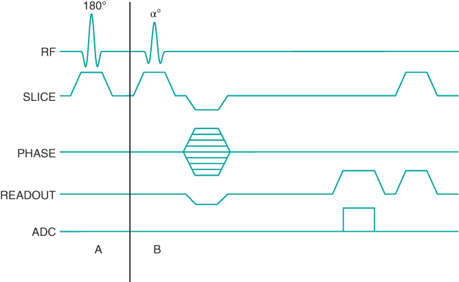
Figure 6.15 Two-dimensional MP sequence timing diagram, T1-weighted. A single 180° inversion RF pulse is applied once per scan (section A). This inversion provides significant T1 weighting to  . The portion of the sequence indicated by
  is repeated for the
  and
and  desired.
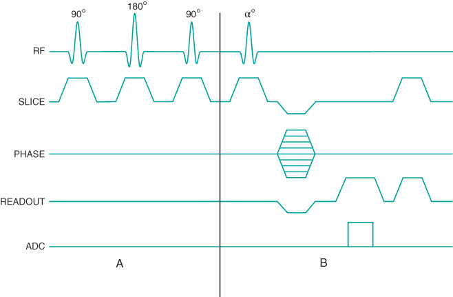
Figure 6.16 Two-dimensional MP sequence timing diagram, T2-weighted. A 90°– 180°– 90° RF pulse train is applied once prior to the data collection scheme (section A). The first two pulses produce T2 weighting to , which is restored to the longitudinal direction by the final pulse prior to the data collection. The portion of the sequence indicated by is repeated for the and desired.
MP gradient echo sequences can be either 2D or 3D techniques. Two-dimensional magnetization prepared techniques are acquired as sequential slice techniques in that all data collection is acquired for a slice following a single set of preparation pulses. The rapid measurement times make them very insensitive to patient motion. These sequences may also be acquired using a segmented k-space in order to increase spatial resolution. Three-dimensional MP techniques typically apply one MP pulse per phase encoding entry  so that the non-steady-state behavior to
  is only present during the loop through the partitions gradient table
  (Figure 6.17). This approach enables the image contrast to be unaffected by the acquisition matrix. It also reduces the number of measured values of
  as the number of
  values is normally smaller than the number of
  values.
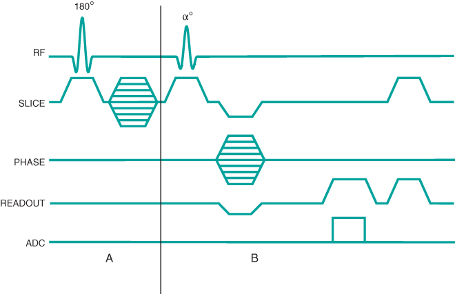
Figure 6.17 Three-dimensional MP sequence timing diagram, T1-weighted. A 180° inversion RF pulse is applied followed by encoding in the slice  direction (section A). This inversion provides significant T1 weighting to
  . The portion of the sequence indicated by
  is repeated for the
  desired. The entire process (A and B) is repeated for the
  and
and  desired.