The Pearson correlation coefficient is a measure of linear association between two interval- or ratio-level variables. Although there are other types of correlation (several are discussed in Chapter 5, including the Spearman rank-order correlation coefficient), the Pearson correlation coefficient is the most common, and often the label “Pearson” is dropped, and we simply speak of “correlation” or “the correlation coefficient.” Unless otherwise specified in this book, “correlation” means the Pearson correlation coefficient. Correlations are often computed during the exploratory stage of a research project to see what kinds of relationships the different continuous variables have with each other, and often scatterplots (discussed in Chapter 4) are created to examine these relationships graphically. However, sometimes correlations are statistics of interest in their own right, and they can be tested for significance and reported as inferential statistics as well. Understanding the Pearson correlation coefficient is fundamental to understanding linear regression, so it’s worth taking the time to learn this statistic and understand well what it tells you about the relationship between two variables. A key point about correlation is that it is a measure of an observed relationship but cannot by itself prove causation. Many variables in the real world have a strong correlation with each other, yet these relationships can be due to chance, to the influence of other variables, or to other causes not yet identified. Even if there is a causal relationship, the causality might be in the opposite direction of what we assume. For these reasons, even the strongest correlation is not in itself evidence of causality; instead, claims of causation must be established through experimental design (discussed in Chapter 18). In this chapter, we discuss the general meaning of association in the context of statistics and then examine the Pearson correlation coefficient in detail.
Ordinary life is full of variables that appear to be associated with or related to each other, and explicating these relationships is a chief task of the sciences. There’s nothing obscure or arcane about thinking about how variables relate to each other, however; people think in terms of associations all the time and often attribute causality to those associations. Parents who order their children to eat more vegetables and less junk food probably do so because they believe there is a relationship between diet and health, and athletes who put in long hours of practice at their sport are most likely doing so because they believe diligent training will lead to success. Sometimes these types of commonsense notions are supported by empirical research, sometimes not, but it seems to be a normal human tendency to take note when things seem to occur together and, often, to believe as well that one is causing the other. As scientists (or just people who understand statistics), we need to be in the habit of questioning whether an apparent association actually exists and, if it does exist, if it is truly causal.
Here are a few examples of conclusions that, although based in some way on observable data, are obviously false:
There is a strong association between sales of ice cream and the number of deaths by drowning, so the reason must be that people are going in the water too soon after eating ice cream, thus getting cramps and drowning.
There is a strong association between score on a vocabulary test and shoe size, so the explanation must be that tall people have bigger brains and hence can remember more words.
There is a strong association between the number of storks in an area and the human birth rate in that area, so obviously storks really do deliver babies.
A town mayor notes a strong correlation between local sports teams winning championships and ticker-tape parades and decides to hold more parades to improve the performance of the local teams.
Here are the real explanations:
Both ice cream consumption and swimming are more common in the hotter months of the year, so the apparent relationship is due to the influence of a third variable, that of temperature (or season).
The data was gathered on schoolchildren and was not controlled for age. We expect that older children will be taller (and have bigger feet) and have acquired larger vocabularies than younger children; hence, the observed association is due to the influence of a third variable, age.
Storks are more common in rural areas, and birth rates are also higher in rural areas, so the association is due to the influence of a third variable, location.
This is reversed causality—the parades are held after the championships are won, so the teams’ successful seasons are the cause of the parades rather than the parades causing the teams to have good seasons.
It’s worth noting that even if two variables have no logical reason at all to be associated, simply by chance they may show some association. This is particularly true in studies with large sample sizes in which a very slight association can be statistically significant, yet have no practical meaning. It’s also worth noting that even among variables that are strongly related, such as smoking and lung cancer, there can be significant variation in that relationship among individuals. Some people smoke for years and never get sick, whereas some unfortunate individuals come down with lung cancer despite never having smoked in their lives.
The scatterplot is a useful tool with which to explore the relationships between variables, and usually, creating scatterplots for pairs of continuous variables is part of the exploratory phase of working with a data set. A scatterplot is a graph of two continuous variables. If the research design specifies that one variable is independent and the other is dependent, the explanatory variable is graphed on the x-axis (horizontal) and the dependent variable on the y-axis (vertical); if no such relationship is specified, it doesn’t matter which variable is graphed on which axis. Each member of a sample corresponds to one data point on the graph, described by a set of coordinates (x, y); if you ever plotted Cartesian coordinates in school, you are already familiar with this process. Scatterplots give you a sense of the overall relationship between the two variables, including direction (positive or negative), strength (strong or weak), and shape (linear, quadratic, etc.). Scatterplots are also a good way to get a general sense of the range of the data and to see whether there are any outliers, cases that don’t seem to belong with the others.
One important reason for inspecting bivariate relationships (relationships between two variables) is that many common procedures assume that these relationships are linear, an assumption that might not be met with any particular pair of variables in any particular data set. Linear in this context means “arranged as a straight line,” whereas any other relationship is considered nonlinear, although we can also apply a more specific description to nonlinear relationships, such as quadratic or exponential. We don’t expect a real data set to perfectly fit any mathematically defined pattern, of course; if the data seems to cluster around a straight line, that’s what we mean by a linear relationship.
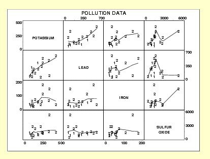
We can also create a scatterplot matrix, which is a display of multiple scatterplots arranged so we can easily see the relationships among pairs of variables. Figure 7-1 displays a scatter plot matrix created by Lloyd Currie of the National Institute of Standards and Technology to inspect the relationships among four pollutants in a data sample: potassium, lead, iron, and sulfur oxide. The scatterplot for each pair of variables is located where the corresponding row and column intersect, so cell (1, 2) (first row, second column) shows the relationship between potassium and lead, cell (1, 3), the relationship between potassium and iron, and so on.
In linear algebra, we often describe the relationship between two variables with an equation of the form:
| In this formula, y is the dependent variable, |
| x is the independent variable, |
| a is the slope, and |
| b is the intercept. |
Note that m is sometimes used in place of a in this equation; this is just a different notational convention and does not change the meaning of the equation. Both a and b can be positive, negative, or 0. To find the value of y for a given value of x, you multiply x by a and then add b. An equation such as this expresses a perfect relationship (given the values of x, a, and b, we can find the exact value of y), whereas equations describing real data generally include an error term, signifying our understanding that the equation gives us a predicted value of y that might not be the same as the actual value. It’s worth looking at some graphs of data defined by equations, however, to get a sense of what perfect relationships look like when graphed; this should make it easier to spot similar patterns in real data.
Figure 7-2 shows the association between two variables, x and y, that have a perfect positive association: x = y. In this equation, b = 0, a = 1, and for every case, the values of x and y are the same. This equation expresses a positive relationship because as the value of x increases, so does the value of y; in a graph of a positive relationship, the points run from the lower left to the upper right.
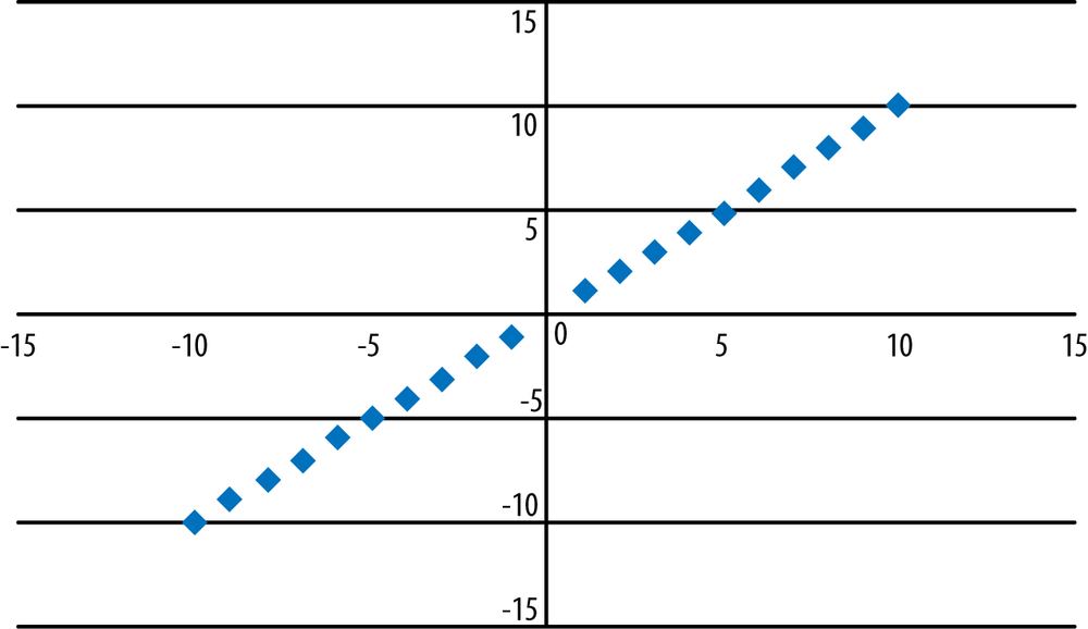
Figure 7-3 shows a negative relationship between x and y: these points are described by the equation y = − x. In this equation, a = −1, b = 0. Note that in a negative relationship such as this one, as the value of x increases, the value of y decreases, and the points in the graph run from the upper left to the lower right.
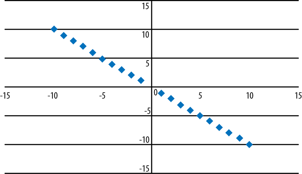
Figure 7-4 shows a positive relationship between x and y as specified by the model y = 3x + 2. Note that this relationship is still perfect (meaning that given the model and a value for x, we can compute the exact value for y) and is represented by a straight line. Unlike the previous two graphs, however, the line no longer runs through the origin (0, 0) because the value for b (the intercept) is 2 rather than 0.

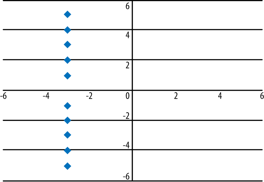
In the previous three graphs, the equation of a straight line indicated a strong relationship between the variables. This is not always the case, however; it’s possible for the equation of a straight line to indicate no relationship between the variables. When one variable is a constant (meaning it always has the same value) while the value of the other variable varies, this relationship can still be expressed through the equation (and graph) of a straight line, but the variables have no association. Consider the equation x = −3, displayed in Figure 7-5; no matter what the value of y, x always has the same value, so there is no association or relationship between the values of x and y. The slope of this equation is undefined because the equation used to calculate the slope has a denominator of 0.
The equation for calculating the slope of a line is given in Figure 7-6.
where x1 and x2 are any two x-values in the data, and y1 and y2 are the corresponding y-values. If x1and x2 have the same value, this fraction has a denominator of 0, so the equation and the slope are undefined.
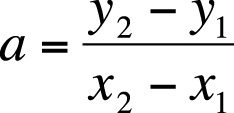
The equation y = −3 also expresses no relationship between x and y, in this case because the slope is 0. In this equation, it doesn’t matter what the value of x is, the value of y is always −3. The graph of this equation is a horizontal line, as shown in Figure 7-7.
In real data sets, we don’t expect that an equation will perfectly describe the relationships among the variables, and we don’t expect the graph to be a perfect straight line, even if the linear relationship is quite strong. Consider the graph in Figure 7-8, which displays almost the same data as shown in Figure 7-4; the difference is that we added some random error to the data so the data no longer form a perfect line. The relationship between x and y is still strongly linear and positive, but we can no longer predict the exact value of y, given the value of x, from an equation. To put it slightly differently, knowing the value of x helps us predict the value of y (versus predicting the value of y without any knowledge of the value of x), but we realize that our predicted value for y might be somewhat different than the actual value in the data set.
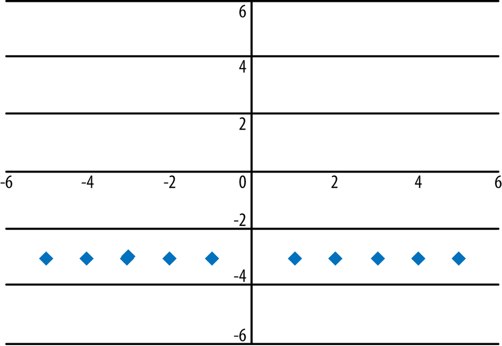
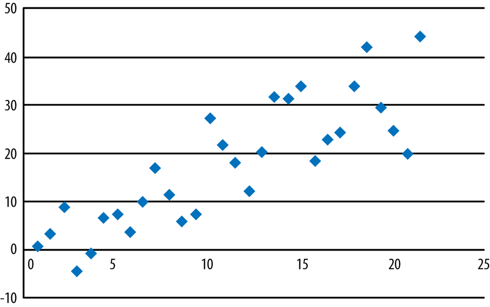
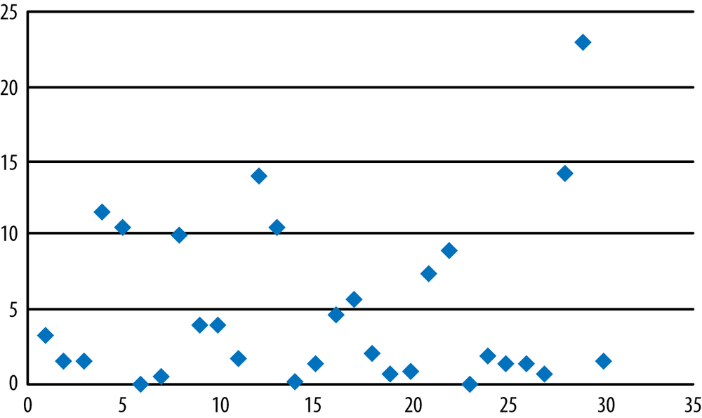
It’s unusual to find as close a relationship between x and y in a real data set as is displayed in Figure 7-8. The data in Figure 7-9 is more typical of what we usually find. Note that even though the points are more scattered than in previous examples, the relationship between x and y still seems to be positive and linear.
Two variables may have a strong relationship that is not linear. To take a familiar example, the equation y = x2 expresses a perfect relationship because, given the value of x, we know exactly what the value of y is. However, this relationship is quadratic rather than linear, as can be seen in Figure 7-10. Spotting this type of strong but nonlinear relationship is one of the best reasons for graphing your data.
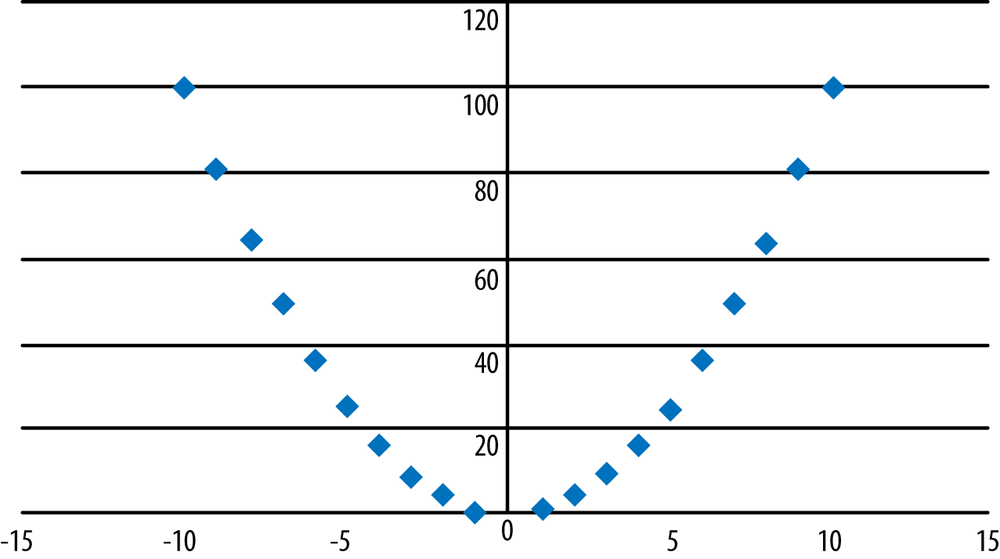
Figure 7-11 shows another common type of nonlinear relationship, a logarithmic relationship defined by the equation y = LN(x), where LN means “the natural logarithm of.”
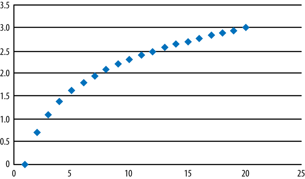
If your data shows a nonlinear relationship, it might be possible to transform the data to make the relationship more linear; this is discussed further in Chapter 3. Recognizing these nonlinear patterns and knowing different ways to fix them, is an important task for anyone who works with data. For the data in Figure 7-10, if we transformed y by taking its square root and then graphed x and √y, we would see that the variables now have a linear relationship. Similarly, for the data graphed in Figure 7-11, if we transformed y to ey and then graphed it against x, we would see a linear relationship between the variables.
Scatterplots are an important visual tool for examining the relationships between pairs of variables. However, we might also want a statistical estimate of these relationships and a test of significance for them. For two variables measured on the interval or ratio level, the most common measure of association is the Pearson correlation coefficient, also called the product-moment correlation coefficient, written as ρ (the Greek letter rho) for a population and r for a sample.
Pearson’s r has a range of (−1, 1), with 0 indicating no relationship between the variables and the larger absolute values indicating a stronger relationship between the variables (assuming neither variable is a constant, as in the data displayed in Figure 7-5 and Figure 7-7). The value of Pearson’s r can be misleading if the data have a nonlinear relationship, which is why you should always graph your data. The labels “strong” and “weak” do not have strict numerical definitions, but a relationship described as strong will have a more linear relationship, with points clustered more closely around a line drawn through the data, than will data with a weak relationship. Some of the definition of strong and weak depends on the field of study or practice, so you will need to learn the conventions for your own field. A few examples of scatterplots of data with different r values are given in Figures 7-12, 7-13, and 7-14 to give you an idea of what different strengths of relationship look like.
Although correlation coefficients are often calculated using computer software, they can also be calculated by hand. The formula for the Pearson correlation coefficient is given in Figure 7-15.
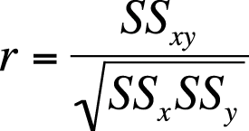
| In this formula, SSx is the sum of squares of x, |
| SSy is the sum of squares of y, and |
| SSxy is the sum of squares of x and y. |
None of the steps in this calculation is difficult, but the process can be laborious, particularly with a large data set. The steps to calculate the sum of squares for x are as follows:
Figure 7-16 shows this written as a formula.
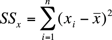
| In this formula, xi is an individual x score, |
 is the sample mean for x, and is the sample mean for x, and |
| n is the sample size. |
This formula makes the meaning of SSx clear, but it can be time-consuming to calculate. The sum of squares can also be calculated using a computational formula that is mathematically identical but less laborious if the calculations must be carried out by hand, as shown in Figure 7-17.
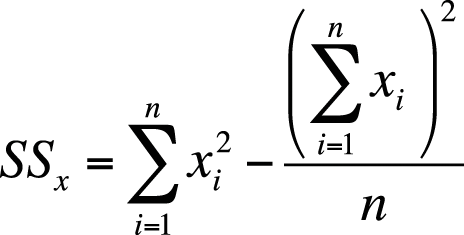
The first part of the computational formula tells you to square each x and then add up the squares. The second part tells you to add up all the x scores, square that total, and then divide by the sample size. Then, to get SSx, subtract the second quantity from the first.
To calculate the sum of squares for y, follow the same process but with the y scores and mean of y.
The process to compute the covariance is similar, but instead of squaring the deviation scores for x or y for each case, you multiply the deviation score for x by the deviation score for y. Written as a formula, it appears as shown in Figure 7-18.
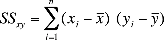
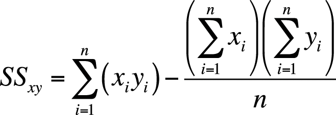
There is also a computational formula for the sum of squares of x and y, as shown in Figure 7-19.
The use of these formulas might become clearer after working through an example. Suppose we drew a sample of 10 American high school seniors and recorded their scores on the verbal and mathematics portions of the Scholastic Aptitude Test (SAT), as shown in Figure 7-20. (Each section of the SAT has a range of 200–800.) To make the data easier to read, we have arranged the scores by verbal score in ascending order, but this is not necessary to perform the calculations.
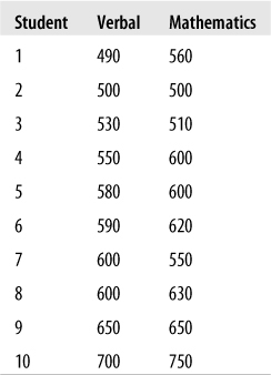
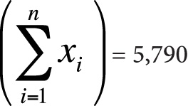
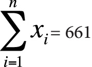
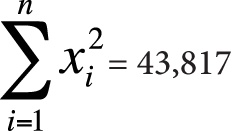
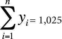
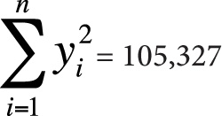
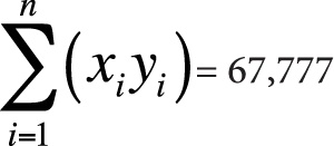
Here is the information you need to use the computational formulas (or to check yourself if you calculated these quantities by hand):
n = 10
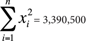
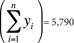
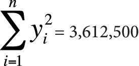
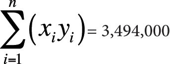
Next, we plug this information into the computational formulas, as shown in Figure 7-21.
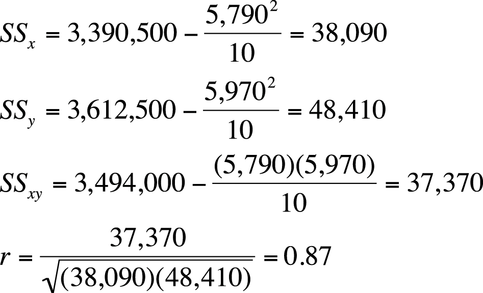
The correlation between the verbal and math SAT scores is 0.87, a strong positive relationship, indicating that students who score highly on one aspect of the test also tend to score highly on the other. Note that correlation is a symmetrical relationship, so we do not need to posit that one variable causes the other, only that we have observed a relationship between them.
We also want to determine whether this correlation is significant. The null hypothesis for designs involving correlation is usually that the variables are unrelated, that is, r = 0, and that is the hypothesis we will test for this example; the alternative hypothesis is that r ≠ 0. We will use an alpha level of 0.05 and compute the statistic in Figure 7-22 to test whether our results are significantly different from 0. This statistic has a t distribution with (n − 2) degrees of freedom; degrees of freedom is a statistical concept referring to how many things can vary in a given design. It is also a number we need to know to use the correct t-distribution to evaluate our results.
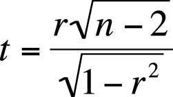
In Figure 7-22, r is the Pearson correlation for the sample, and n is the sample size.
For our data, the calculations are shown in Figure 7-23.
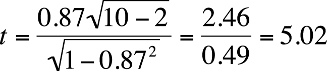
According to the t-table (Figure D-7 in Appendix D), the critical value for a two-tailed t-test with 8 degrees of freedom at α = 0.05 is 2.306. Because our computed value of 5.02 exceeds this critical value, we will reject the null hypothesis that the SAT math and verbal scores are unrelated. We also calculated the exact p-value for this data by using an online calculator and found the two-tailed p-value to be 0.0011, also indicating that our result is highly improbable if the verbal and math scores are truly unrelated in the population from which our sample was drawn.
The correlation coefficient indicates the strength and direction of the linear relationship between two variables. You might also want to know how much of the variation in one variable can be accounted for by the other variable. To find this, you can calculate the coefficient of determination, which is simply r2. In our SAT example, r2 = 0.872 = 0.76. This means that 76% of the variation in SAT verbal scores can be accounted for by SAT math scores and vice versa. We will expand further on the concept of the coefficient of determination in the chapters on regression because very often one of the purposes in building a regression model is to find a set of predictor variables that can account for a high proportion of the variation in our outcome variable.
Problem
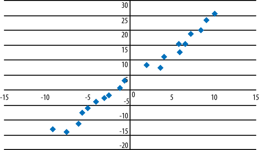
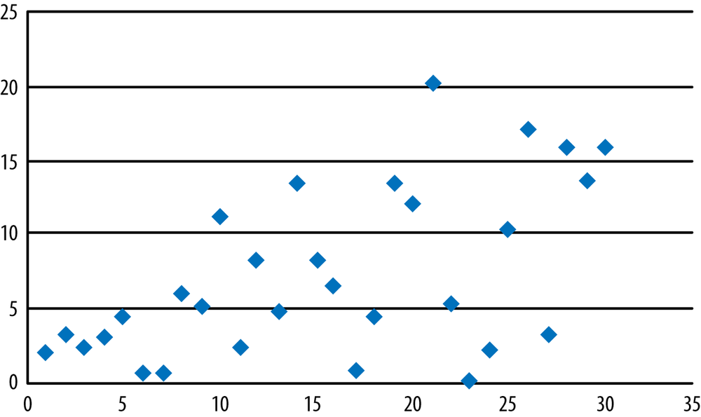
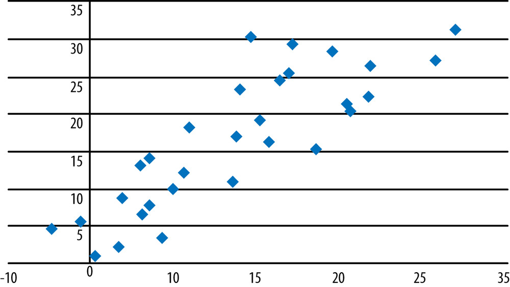
Which of the following scatterplots (Figures 7-24, 7-25, and 7-26) suggest that the two graphed variables have a linear relationship? For those that do, identify the direction of the relationship and guess its strength, that is, the Pearson’s correlation coefficient for the data. Note that no one expects you to be able to guess an exact correlation coefficient by eye, but it is useful to be able to make a plausible estimate.
Solution
Strong positive linear relationship (r = 0.84).
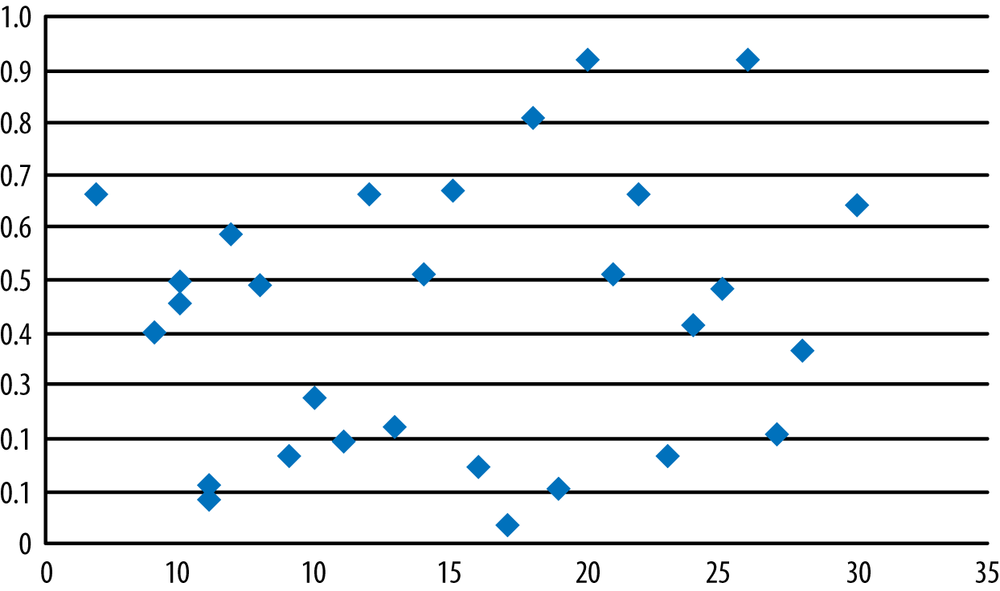
Weak relationship (r = 0.11).
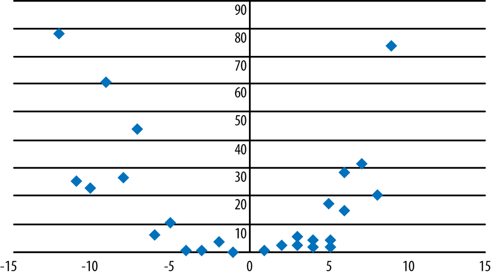
Nonlinear, quadratic relationship. Note that r = –0.28 for this data, a respectable correlation coefficient, so that without the scatterplot, we could easily have missed the nonlinear nature of the relationship between these two variables.
Problem
Find the coefficient of determination for each of the data sets from the previous problem, if appropriate, and interpret them.
Solution
r2 = 0.842 = 0.71; 71% of the variability in one variable can be explained by the other variable.
r2 = 0.112 = 0.01; 1% of the variability in one variable can be explained by the other variable. This result points out how weak a correlation of 0.11 really is.
r and r2 are not appropriate measures for variables whose relationship is not linear.
Problem
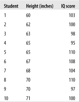
Several studies have found a weak positive correlation between height and intelligence (the latter as measured by the score on an IQ test), meaning that people who are taller are also on average slightly more intelligent. Using the formulas presented in this chapter, compute the Pearson correlation coefficient for the data presented in Figure 7-27, which represent height (in inches) and scores on an IQ test for 10 adult women. Then test the correlation for significance (do a two-tailed test with alpha = 0.05), compute the coefficient of determination, and interpret the results. For the sake of convenience, we will designate height as the x variable and IQ score as the y variable.
Solution
The calculations are shown in Figures 7-28 and 7-29.
n = 10
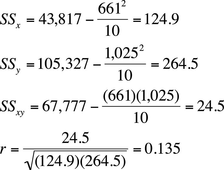
Coefficient of determination = r2 = 0.018
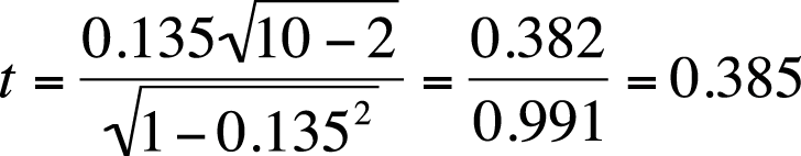
In this data, we observe a weak (r = 0.135, r2 = 0.018) positive relationship between height and IQ score; however, this relationship is not significant (t = 0.385, p > 0.05), so we do not reject our null hypothesis of no relationship between the variables.
If you are interested in this issue, see the paper by Case and Pearson in Appendix C; although primarily concerned with the relationship between height and income, it also summarizes research about height and intelligence.