Often, one of the responsibilities of a statistician is to design research studies. To do this well, you must be familiar with the different types of research designs, know their strengths and weakness, and be able to draw on this knowledge to design studies to examine different types of questions. You also need to be familiar with the customs and practices of your profession, such as what type of study is generally used for a particular type of data or to answer a particular type of question. Research design is a larger subject than can be covered in a single chapter, so this chapter can only introduce the major issues in designing research studies and discuss some of the most common types of designs. Typically, designing a study involves compromise between what the researcher would ideally like to do and what is feasible, and the choice and execution of a design should be guided by consideration of what is most important to the research question and the traditions and standard practices in the relevant field of study. We’d all love to conduct research that is both perfectly controlled (meaning the experimenter can manipulate or otherwise control all the factors relevant to the research) and perfectly naturalistic (meaning that whatever is being measured is being so in a realistic, natural environment). However, the characteristics of control and naturalism are often in competition with each other, and learning to judge how much to emphasize one versus the other is one aspect of becoming a competent research designer. One influence on these decisions is the purpose of the research. Is it to determine some underlying cause for a phenomenon, as is common in science, or to optimize the yield or output for a specific process while minimizing expense and effort, as is often the case in business and technology research? Practical and ethical considerations also come into play—some research designs can simply be impossible to execute, prohibitively expensive, or considered unethical—and the researcher must be aware of community as well as scientific standards concerning the ethical conduct of research.
Research designs can be divided into three types: experimental, quasi-experimental, and observational. For a design to be experimental, subjects must be randomly assigned to groups or categories. The classic experimental design is the randomized controlled trial used in medicine, in which subjects are randomly assigned to experimental and control groups, administered some treatment, and the outcomes collected for both groups. The controlled experiment is considered the strongest type of research design as far as drawing conclusions from the results of research (in fact, some refer to the results from experimental controlled trials as the gold standard of evidence), but it is not always possible or practical to conduct this type of research. The next strongest design is the quasi-experimental, in which some sort of control or comparison group is used, but subjects are not randomly assigned to experimental and control groups. In an observational study, the researcher makes no assignments to groups or treatments but observes the relationships of different factors and outcomes as they exist in the real world. Although experimental designs are preferred for their ability to minimize systematic error or bias (a topic discussed in Chapter 1), quasi-experimental and observational designs have the advantage of minimizing experimenter intrusion into natural processes. This is important particularly in studies with human subjects because human behavior is highly situational, and a person’s behavior in a lab situation where she knows she is being observed might be quite different from the way she behaves in her normal life. Again, decisions about which kind of design to use depend on what is most important for the research and possible from a practical and ethical point of view.
A factor is an independent variable (predictor variable) in a research design, that is, a variable that is believed to exert some influence on the value of a dependent variable (outcome variable) in the design. Often, experimental designs include multiple factors. If you were studying childhood obesity, factors that you might include in your study include parental obesity, poverty, diet, physical activity level, gender, and age. Some researchers call any research design that includes more than one factor a factorial design; others reserve this terms for designs in which all possible combinations of factors appear, also called a fully crossed or fully factorial design. You might be interested in the influence of each of these variables alone (main effects) and in their joint influence (interaction effects). You might believe that diet plays a role in child obesity (a main effect) but that the influence of diet is different depending on whether the study subject is male or female (an interaction effect).
Studies can also be classified by the relationship between the time when events occurred and the time when information about them is collected for use in the study. In a prospective study, data is collected from the starting point of the study into the future. A group that shares a common point of origin, such as their time of entry into the study or their year of birth, is called a cohort, so a prospective cohort study is one that follows a group of people (or other objects of study) forward in time, collecting information about them for analysis. In contrast, a retrospective study collects information about events that occurred at some time before the study began.
In terms of data types, researchers often differentiate between primary and secondary data. Primary data is collected and analyzed for a particular research project, whereas secondary data is collected for some purpose and later analyzed for some other purpose. There are tradeoffs between the two, and some researchers might work only with one or the other, other researchers with both. The greatest advantage of primary data is its specificity; because it is collected as part of the project that will also analyze it, it can answer the specific needs of a particular research project. In addition, the people analyzing primary data are most likely familiar with when and how it was collected. On the downside, because data collection is expensive, the scope of data collected by any one researcher or research team is limited. The greatest advantage of secondary data is scope. Because secondary data sets are often collected by governmental entities or major research institutions such as the National Opinion Research Center (located in Chicago), they are often national or international in scope and may be collected over many years, achieving a breadth of coverage of which individual researchers can only dream. The downsides with secondary data are that you have to take the data as it is, it might not correspond exactly to the purposes of your study, and there might be limitations on what data you are allowed to use. (For instance, confidentiality concerns can mean that individual-level data is not available.)
A final consideration is the unit of analysis in a study. The unit of analysis (further discussed in Chapter 17) is the primary focus of a research study. In human research, the unit of analysis is often the individual person, but it also can be collections or populations of individuals who are members of some larger unit such as a school, a factory, or a country. Studies in which the unit of analysis is populations rather than individuals are known as ecological studies. Although ecological studies can be useful in identifying potential areas of research (the relationship between a high-fat diet and heart disease) and are relatively cheap to carry out because they generally rely on secondary data, conclusions from ecological studies must be interpreted with caution because they are subject to the ecological fallacy. The ecological fallacy refers to the belief that relationships that exist at one level of aggregation (say, the country) also exist at a different level (the individual). In fact, the strength and/or direction of the relationship analyzed with one unit of analysis can be quite different when the same data is analyzed using a different unit of analysis. A classic paper by W.S. Robinson, listed in Appendix C, demonstrated the ecological fallacy with a series of analyses of the relationship between race and literacy in the United States at different levels of geographic aggregation.
Cook and Campbell Notation
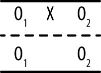
Thomas D. Cook and Donald T. Campbell developed a style of notation for research design that has been adopted and adapted by many researchers. The key elements of this notation include O for an observation (collection of data), X for an intervention, R for randomization, a dashed line to indicate groups formed without randomization, and subscripts to indicate the order of observations or interventions. In Cook and Campbell notation, a randomized pretest-posttest design with an experimental and control group would be notated as shown in Figure 18-1.
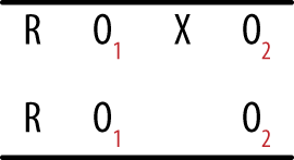
This notation means that subjects are randomly assigned to treatment and control groups, initial measurements are taken from both groups, a treatment or intervention is delivered to the treatment but not to the control groups, and then measurements are taken again on both groups. This type of design is common in medical studies, in which the experimental intervention is a drug or other type of treatment; the control group does not receive this intervention but receives either standard treatment or no treatment. In the latter case, the members are sometimes called the placebo group.
In contrast, a quasi-experimental pretest-posttest design is notated as shown in Figure 18-2.

The difference in the quasi-experimental design is that subjects are not randomly assigned to groups. Often in this type of design, preexisting groups such as a classroom or a school are used rather than the random assignment of individuals to groups; the group that does not receive the intervention is called the comparison group.
Cook and Campbell’s notation is simple and flexible, which explains its continued popularity. They also did a great deal to call attention to the use of weak designs in educational and social research and to point out the problems with trying to draw any conclusions from the data produced from poorly designed studies. Their catalogue of threats to validity and threats to reliability is an excellent reminder to researchers of the many factors that can bring into question the conclusions of even well-designed studies. Cook and Campbell’s classic textbook on research design has been updated by William Shadish and is listed in Appendix C.
Observational studies are generally conducted when it is not possible to conduct an experimental study or when collecting information from subjects in a natural environment is more valued than the control that is possible in an experimental setting. For an example of the first reason, consider research into the effects of cigarette smoking on human health. This research can be done only through observational studies because it would be unethical to assign some people to take up tobacco smoking, a practice known to be harmful to human health. Instead, we observe people who choose to smoke and compare their health outcomes with those of people who do not smoke. As an example of the second reason, consider research into disruptive behavior by primary school students. Because the disruptive behavior might be set off by specific triggers that occur in the school setting, researchers might choose to observe students in their usual classrooms rather than bringing them into the lab for observation.
One well-known type of observational study is the case control design, often used in medicine to study diseases that are rare or take a long time to develop. A prospective cohort study is an impractical design to study a rare or slow-developing disease because you would need to follow an extremely large cohort to have a chance of a sufficient number developing the disease in question, and the study might have to last 20 or 30 years (or longer) before members of the cohort begin to be diagnosed with the disease. A case control design circumvents these difficulties by beginning with people who have the disease (the cases), then collecting another group of people (the controls) who do not have the disease but who are similar in other ways to the cases. Case control research generally focuses on identifying factors (diet, exposure to occupational chemicals, smoking habits, use of prescription drugs) that differentiate the cases and controls in the hope of finding a key factor or factors that could explain why the cases have the disease and the controls do not. Some would classify the case control design as quasi-experimental because it includes a control group; however, the term “quasi-experimental” is more often used to describe prospective experiments in which groups are designated and then observed going forward in time.
The strength of a case-control study rests in large part on the quality of the match between cases and controls; ideally, the controls should be like the case in every way except that they do not have the disease. As a practical matter, matching is more often done on just a few variables that are considered important in terms of risk for the disease such as age, gender, presence of comorbidities (other diseases), and smoking habits. A recent method to improve matching is the use of a propensity score, which uses various factors to predict the probability of a given individual being a case or a control. Donald Rubin and Paul Rosenbaum first proposed use of the propensity score; see Appendix C for the citation to the article in which they introduced this approach.
A cross-sectional design involves a single time of observation; the most common example of cross-sectional design is a survey that collects data through a questionnaire or interview. The data collected by this type of design is like a snapshot that captures the state of the individuals surveyed at a particular moment. Although cross-sectional studies can be extremely helpful in tracking population trends and in collecting a wide variety of information from a large number of people, they are less useful in terms of establishing causality because of the lack of temporal sequence in the data. For instance, a cross-sectional survey might ask how many hours of television per week a person watches and about his height and weight. From this information, a researcher can calculate the BMI (body mass index, a measure of obesity) for all the individuals surveyed and investigate the association between television viewing habits and obesity. She could not, however, claim that excessive television watching causes obesity because all the data was collected at one point in time. In other words, even if the data shows that obese people on average watch more television than thin people, it can’t tell you whether the obese people watched a lot of television and then became obese, or they became obese first and then took up watching television because more active pursuits became too difficult.
A cohort study can also be observational. A good example is the famous Framingham Heart Study, which began following a cohort of more than 5,000 men living in Framingham, Massachusetts (U.S.) in 1948 to identify factors associated with cardiovascular disease (heart disease). The men in the study, who were between the ages of 30 and 62 and without symptoms of cardiovascular disease at the start of the study, have returned every two years to allow researchers to gather data from them based on lab tests, a physical exam, and a medical history. The study is still active and has enrolled two subsequent cohorts, including spouses, children, and grandchildren of the original participants. The Framingham Heart Study has made important contributions toward identifying major risk factors for heart disease (high blood pressure, smoking, diabetes, high cholesterol, and lack of physical activity) as well as the relationships between heart disease and factors such as age, blood triglycerides, and psychosocial factors.
The major criticism of observational studies is that it is difficult if not impossible to isolate the effects due to individual variables. For instance, some observational studies have noted that moderate wine consumption is associated with a higher level of health as compared to abstinence, but it is impossible to know whether this effect is due to the wine consumption or to other factors characteristic of people who drink wine. Perhaps wine drinkers eat better diets than people who don’t drink at all, or perhaps they are able to drink wine because they are in better health. (Treatment for certain illnesses precludes alcohol consumption, for instance.) To try to eliminate these alternative explanations, researchers often collect data on a variety of factors other than the factor of primary interest and include the extra factors in the statistical model. Such variables, which are neither the outcome nor the main predictors of interest, are called control variables because they are included in the equation to control for their effect on the outcome. Variables such as age, gender, socioeconomic status, and race/ethnicity are often included in medical and social science studies, although they are not the variables of interest, because the researcher wants to know the effect of the main predictor variables on the outcome after the effects of these control variables have been accounted for. Such corrections after the fact are always imperfect, however, because you can never know all the variables that might affect your outcome, and there are practical limitations to how much data you can collect and how much you can include in any analysis.
Although observational studies are generally considered weaker in terms of statistical inference, they have one important characteristic: response variables (such as human behavior) can often be observed within the natural environment, enhancing their ecological validity, or the sense in which what is being observed has not been artificially constrained by engaging in a narrowly defined experimental paradigm. Going one step further, some observational studies use participant observation methods in which a researcher becomes involved in the activity under study. If this participation is hidden from the actual participants, ethical issues can arise around the use of deception, so safeguards must be built into the study to see that no inadvertent harm occurs because of the experimental procedures.
Quasi-experimental studies are similar to experimental studies in that they use a control or comparison group but differ in that participants are not randomly assigned to those groups. Quasi-experimental designs are often used in field research (research in which data is collected in a natural setting as opposed to the laboratory or other obviously experimental setting) and are particularly popular in education and social science research, in situations in which experimental designs would often be impractical. For instance, if you want to study the effects of a new approach to teaching math, you can assign one preexisting classroom to use the new method and another to continue using the old method; at the end of the school year, you would then compare student achievement in the two classrooms. This is not an experimental design because students were not randomly assigned to the treatment (new method) and control (old method) groups, but a true experimental design would be impractical in a school setting. Instead, selecting a comparable group of students to use as a comparison group to the students who get the experimental treatment (the new method of teaching) is a compromise solution and is better than having no source of comparison at all.
The usefulness of a quasi-experimental design might be clearer if we contrast it with some weaker designs often used out of expediency. The terminology and notation used in this section was developed by Thomas D. Cook and Donald T. Campbell (see the sidebar Cook and Campbell Notation and the Shadish reference in Appendix C), and it has become a widely used research design. Three particularly weak yet commonly used designs are the one-group posttest-only design, the posttest-only nonequivalent groups design, and the one-group pretest–posttest design. As Cook and Campbell note, results from studies using these designs could be due to so many reasons other than the factor of interest that it is difficult to draw any conclusions from them.
In the posttest only design, an experimental treatment is delivered and data collected on the group that received the treatment, as shown in Figure 18-3.
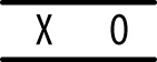
This design is as simple as it looks; you deliver an intervention to a single group and then observe the members once. It can be useful if information is available from other sources about the condition of the experimental group before the intervention, and it may be used in the very early stages of research to gather descriptive information used to create a stronger design for the main study. However, without contextual information, this design amounts to little more than “We did some stuff, and then we took some measurements.” True enough, but what is the value of the resulting data? It is difficult, if not impossible, to justify drawing causal inferences from this design because so many factors other than the intervention could also be responsible for any observed outcomes. Without knowing the precise state of the group before the intervention, it is difficult to say anything about how the members might have changed, and without a control group, it is not possible to say that the changes were due to the intervention. Other possible explanations include chance, the influence of events outside the study, maturation (normal growth processes; this cause is particularly relevant when studying children and adolescents), and the effects of being studied.
The posttest-only non-equivalent groups design adds one refinement to the one-group posttest-only design: a comparison group that does not receive the intervention but is measured or observed at the same time as the intervention group, as shown in Figure 18-4.
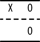
This design might provide useful preliminary descriptive data if information is available from another source about the state of the two groups before administration of the intervention, and the use of a comparison group (ideally one as similar as possible to the experimental group, such as a comparable class within the same school) provides some information that might help place the measurements in context. Data from the comparison group also helps eliminate some alternative explanations such as maturation (assuming the two groups are the same age and have roughly comparable experience regarding whatever is being measured). However, differences observed between the experimental and comparison groups could be due to initial differences between the two groups rather than to the intervention, and the lack of random assignment, as well as the lack of pretest information, makes it difficult to eliminate this explanation for any differences observed between the groups.
The one-group pretest-posttest design uses only one group but adds an observation (the pretest) before the intervention is delivered, as shown in Figure 18-5.
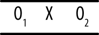
Although the collection of information about the experimental group prior to the intervention is certainly useful, it is still not possible to draw causal inference from data collected from this type of design. The reason is that so many other explanations for the observed results are possible. Besides obvious issues such as maturation and influence from outside events, statistical regression (also called regression to the mean) must always be considered with this type of design, particularly if the experimental group was selected due to high or low performance on some measure related to the purpose of the study. Suppose a group of children who score poorly on a reading test (the pretest) is given extra coaching in reading (the intervention) and then tested again (the posttest). They may well perform better on the posttest than on the pretest, but ascribing this change to the influence of the intervention requires a leap of faith not supported by the study design because all measurements include a component of random error. (This is further discussed in Chapter 16.) For instance, each student in our hypothetical study has a true level of competency in reading, but any particular measurement of his reading competency (the score on a reading test) includes some error of measurement that might make his observed score higher or lower than the true score that reflects actual competency. Thus, a student who scores low on one reading exam might score higher on the next simply due to this random error of measurement, without her level of competency in reading having changed at all. If a study group is selected for its extreme scores (for instance, children who perform poorly on a reading test), the probability of regression to the mean resulting in higher scores on a second testing occasion is increased.
Cook and Campbell present many quasi-experimental designs that are preferable to these three (see the Shadish, Cook, and Campbell book in Appendix C for more on this topic); all represent attempts to improve control in situations when it is not possible to include random assignment to groups. One simple example is the pretest-posttest design with comparison group illustrated in Figure 18-6.
In this design, a comparison group is selected that is similar to the experimental group, but subjects are not assigned randomly to either group; instead, most often, preexisting groups are used. Measurements are taken on both groups, the intervention is delivered to the experimental group, and measurements are taken on both groups again. The main downside to this design is that without random assignment, the experimental and comparison groups might not be truly comparable; administering the pretest to both groups helps but does not completely overcome this difficulty. Other threats to this design include the fact that simply receiving any intervention can cause a difference in the outcome (for this reason, the control group sometimes receives a different intervention not believed to affect the outcome) and that the two groups might have different experiences outside of the experimental context. Different classrooms have different teachers; different towns might have different economic conditions, and so on.
The interrupted time series shown in Figures 18-7 and 18-8 is a quasi-experimental design that might or might not include a comparison group.

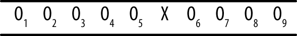
The number of observations can vary from one study to another, but the basic idea is that a series of measurements is recorded over a period of time, an intervention is delivered, and then another series of measurements is recorded over a period of time. This design is often used to judge the effects of legal or social policies that affect large groups of people, such as passage of a law requiring drivers to wear seat belts or increasing fees charged to households for waste disposal. Multiple measurements are taken over a period of time before the intervention to establish a baseline level and again after the intervention to establish the new level. Multiple measurements are necessary to control for the natural fluctuation of the phenomena. For instance, even without any change in laws, the number of traffic accidents varies from one month to the next. Ideally, the baseline measurements should be stable around a particular value, and the post-intervention measurements should be stable but around a different value and in the expected direction. The addition of a comparison group to this design strengthens the researcher’s ability to draw conclusions because it can help control for nonintervention influences that might influence the results. (A public conservation campaign might influence people to begin recycling and composting, independent of the effect of the higher trash disposal fees.)
Suppose a state is concerned about the number of traffic deaths and decides to lower the speed limit on highways, a decision that it believes will result in fewer deaths. Because the reduced speed limit will affect everyone who drives in that state, it is not possible to have a control group; instead, a neighboring state with similar demographics and traffic death rates is chosen to serve as a comparison group. Data from this study is presented in Figure 18-9.
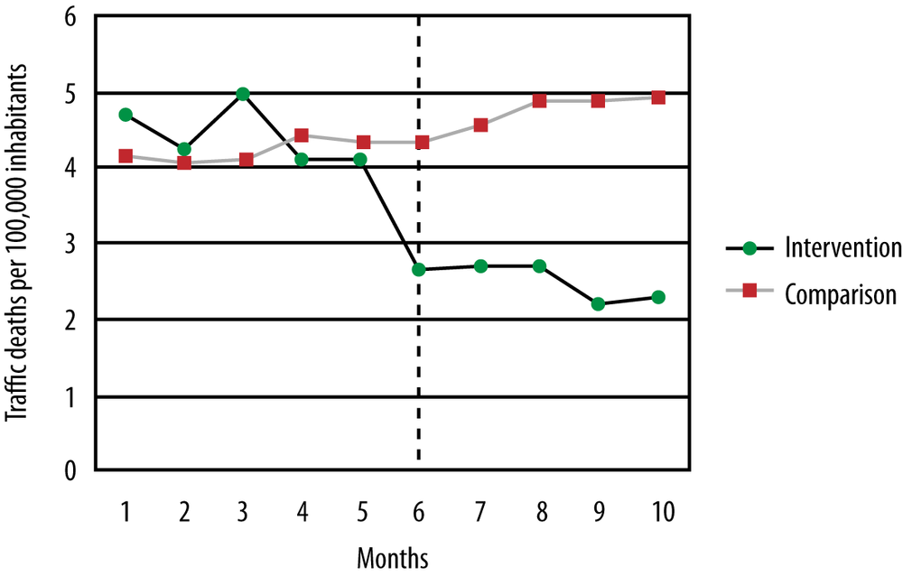
The black line represents traffic deaths in the intervention state, the grey line those in the comparison state; the vertical dotted line shows when the intervention (the new speed limit) took effect. As can be seen, the two states had comparable rates of traffic deaths in the five months preceding the intervention; then deaths dropped in the intervention state and became stable around a new, lower level, as would be expected if the law were effective in reducing traffic deaths. No such change was observed in the comparison state (in fact, the rate of traffic deaths might have risen slightly), giving support to the contention that the law, rather than any other influence, was responsible for the observed decline in traffic deaths. Of course, we would also conduct a statistical investigation to see whether the change was significant, but the graph suggests that the intervention did have an effect in the desired direction.
Experimental studies provide the strongest evidence for causal inference because a well-designed experiment can control or eliminate the influence of many sources of variation, making us more comfortable in asserting that observed effects are due to the experimental intervention rather than to any other cause. There are three elements to an experimental study, and the configuration of the design can range from the very simple to the very complex:
- Experimental units
The objects under examination. In human experiments, units are generally referred to as participants, given their active engagement in the experimental process.
- Treatments
The interventions applied to each unit in the experimental setting.
- Responses
The data collected after the treatment has been delivered that form the basis for evaluating the effects of the treatment.
Besides the treatments that are the focus of the study, other variables might be believed to affect the responses. Some of these are characteristics of the experimental subjects; in the case of human subjects, they might include qualities such as age and gender. These characteristics can be of interest to the researchers (it might be hypothesized that a treatment is more successful with males than with females), or they might simply be nuisance variables or control variables that might obscure the relationship between treatment and response. For nuisance or control variables, you want to neutralize their effects on the response variables, and normally this is done by having approximately equal representation on the important nuisance or control variables in the experimental and control groups. Normally, random assignment will make the distribution of characteristics such as gender and age approximately equal in each group; if this is not sufficient, matching or blocking procedures can also be used, as described later.
In some experimental designs, a comparison is made between a baseline measurement for each unit before treatment and the measurement for the unit after treatment (also known as pretest and posttest responses). This type of design is known as a within-subjects design and provides a high degree of experimental control because measurements on units are made only with themselves; participants act as their own controls. The example of the matched-pairs t-test discussed in Chapter 6 is an example of a within-subjects design. In a between-subjects design, comparisons are made between different units, and frequently, the units are matched on one or more characteristics to ensure the least confounded comparison of the treatment on units from the control and experimental groups.
The goal of an experiment is to determine the effect of an experimental treatment; this is often measured by the differences in response values for members of the treatment and control groups. It’s important to use good procedures for allocating experimental units to treatment and control; indeed, the method of allocating units is a basic difference that separates experimental from observational studies. A major goal of any experimental design is to minimize or preferably eliminate systematic errors or biases in the data collected.
For many reasons—including ethical and resource considerations—the amount of data collected should be minimally sufficient to answer a particular research question. The use of effective sampling and power calculations (discussed in Chapter 16) ensures that the smallest number of experimental units is subjected to experimentation and that a result can be achieved with the least cost and effort.
An effective research design makes analysis much easier later on. For example, if you design your experiment so that you will not encounter missing observations, you will not need to worry about coding missing data and any limitations of interpretation from your results that might subsequently arise (a topic explored further in Chapter 17), including the biases that might accompany nonrandom missing data.
Statistical theory is flexible to the extent that many sophisticated types of designs are mathematically possible, but in practice, most statistics (and therefore designs) are structured according to the requirements of the general linear model. This simplifies analysis because many techniques, such as correlation and regression, are based on this model. However, to make valid use of the general linear model, an experiment must be designed with several important factors in mind, including balance and orthogonality.
Balance means that treatments are administered in equal numbers within each experimental block; they will occur with the same frequency. Balanced designs are more powerful than unbalanced designs for the same number of subjects, and an unbalanced design can also reflect a failure in the process of subject allocation. Randomization of group allocation, blinding, and identifying biases are all mechanisms for ensuring that balance is maintained; these are discussed later in this chapter.
Orthogonality means that the effects of different treatments can be independently estimated without interfering with each other. For example, if you have two treatments in an experiment and you build up a statistical model that measures their effects on experimental units, you should be able to remove either treatment from the model and get the same answer for the remaining treatment.
None of this is as complicated as it first sounds, and if you stick to some well-known recipes and templates for factorial design, you won’t need to worry about more exotic exceptional cases.
So, you want to run an experiment, but where do you start? This section offers a general outline of the research process, roughly in the order in which you need to carry out each step, but your plan should also consider how experiments such as the one you are planning are usually approached in your field of work or study. Stand on the shoulders of giants, in other words; if you are running experiments in a scientific discipline, look at some articles from research journals in that specific discipline, and ensure that the designs and analyses that you carry out are consistent with what others are using in the field. The process of peer review, although not flawless, ensures that the methodology used in an article has been vetted by at least two experts. If you have an advisor or supervisor, you might ask her for advice as well—there’s no sense in reinventing the wheel. In industry or manufacturing, it might be harder to find guidance, but company technical reports and previous analyses should provide some previous examples—even if they have not been peer-reviewed—that you might find instructive.
Having said that, you will be surprised at just how much variation and urban mythology surrounds experimental design, so let’s walk through the steps one by one:
Identify the experimental units you want to measure.
Identify the treatments you want to administer and the control variables you will use.
Specify treatment levels.
Identify the response variables you will measure from the experimental units.
Generate a testable hypothesis that predicts what effect the treatment will have on the response variables.
Run the experiment.
Analyze the results.
Design (steps 1–5) can seem easy when looked at in the abstract, but let’s look at each step in detail to see what’s really involved.
Recall that statistics are calculated on samples and are estimates of the parameters of the populations from which the samples were drawn. To ensure that these estimates are accurate estimates, most statistical procedures rely on the assumption that you have selected these units randomly from the population. (Matched and paired designs are an obvious exception to this rule.) Bias can very easily creep into a design at this first stage, and yet, circumstances might dictate that bias cannot be easily avoided.
For example, many research studies in psychology use undergraduate psychology students as participants. This serves two purposes. First, as part of their coursework, students are exposed to a wide variety of experimental designs and get to experience firsthand what is involved in running an experiment; second, the participant group is easily accessible for psychological researchers. In some ways, the homogeneity of the students serving as the subject pool provides a type of control because the participants can be of similar ages, have an even split in terms of sex, come from the same geographical area, have similar cultural tastes, and so on. However, they are not a random sample from the general population, and this might limit the inferences you can make from your data. Research papers based on a sample of college students might tell us more about the behavior of college students than about the population at large; whether this is an important distinction depends on the type of research being conducted. This problem is not limited to psychology; despite the expectations of random selection of subjects, in practice, researchers in many fields select their subjects nonrandomly. For instance, medical research is often performed with patients in a particular hospital or people who receive care at particular clinic, yet the results are generalized to a much larger population; the justification is that biological processes are not dependent on matters of geography, so results from one set of patients should generalize to similar patients as well. It’s important to know what the expectations and standard practices are in your particular field in terms of sample selection and the validity of generalizing results from a sample because no one rule applies in all fields of study.
What is meant by random selection in this context? Imagine a lottery in which every citizen of a country receives a ticket. All the tickets are deposited in a large box, which is mixed by rotation through many angles. An assistant is then asked to pick one ticket by placing his hand in the box and selecting the first ticket he touches. In this case, every ticket has an equal chance of being selected. If you needed 100 members for a control and 100 for an experimental group, you could select them using a similar process by which the first 100 selections are allocated to a control group, and the next 100 are allocated to the treatment group. Of course, you could alternate selection by allocating the first ticket to a control group, the next to the treatment group, the third to a control group, and so on. If the sampling is truly random, the two techniques will be equivalent. It’s important, for the selection to be random, that the allocation of any particular individual must be truly independent of the selection of any of the others.
Different procedures for drawing samples are discussed further in Chapter 3. The main point to remember here is that in real-world situations, it is often not possible or feasible to draw a random sample from the population, and practical concerns dictate that your sample will be drawn from a population smaller than the one you wish to generalize to (that you believe your results apply to). This is not a problem if you are clear about where and how your sample was obtained. Imagine that you are a microbiologist interested in examining bacteria present in hospitals. If you use a filter with pores of diameter one µm (micrometer), any bacteria smaller than this will not be part of the population that you are observing. This sampling limitation will introduce systematic bias into the study; however, as long as you are clear that the population about which you can make inferences is bacteria of diameter greater than one µm, and nothing else, your results will be valid. In reality, we often want to generalize to a larger population than we sampled from, and whether we can do this depends on a number of factors.
In terms of medical or biological research, generalizing far beyond the population that was sampled is common because of the belief that basic biological processes are common to all people. For this reason, the results of medical research conducted with patients in one hospital can be assumed to apply to patients all over the world. (Of course, not every medical result generalizes this easily.) Another fact to keep in mind is that by explicitly stating the limitations of your sample, you can produce valid results that add to the general body of knowledge. Because many such studies are conducted in a particular field, it might be possible to generalize the results to the general population as well. For example, carrying out tests of reaction time to English words might be used to make inferences about the perceptual and cognitive processing performance of English-speaking people. Subsequent experiments aimed at increasing the possibility of generalizing the finding might include the same experiment but with German words displayed to German speakers, French words to French speakers, and so on. Indeed, this is the way more general results are built up in science.
Treatments are the manipulations or interventions that you want to perform to demonstrate an experimental effect. Suppose a pharmaceutical company has spent millions of dollars developing on a new smart drug, and after many years of testing in the lab, it now wants to see whether it works in practice. It sets up a clinical trial in which it selects 1,000 participants by randomly selecting names from a national phone book, giving a truly representative sample of the population on significant parameters such as age, gender, and so on. Luckily, it has a 100% success rate in recruiting participants for the study (everyone wants to be smarter, right?), so they don’t have to worry about the selected sample refusing to participate or dropping out (both of which could introduce bias into the sample). All participants will be tested on the same day in identical experimental conditions (exactly the same location, temperature, lighting, chair, desk, etc.). At nine in the morning, participants are administered an intelligence test by computer; at noon, they are given an oral dose of the smart drug with water; and at 3 P.M., they sit for the same intelligence test again. The results show an average increase in intelligence of 15%! The company is ecstatic, and it releases the results of the test to the stock exchange, resulting in a large increase in the company’s share price. Nevertheless, what’s wrong with the treatments administered in this experiment?
First, because everyone was tested in exactly the same place and under exactly the same experimental conditions, the result cannot be automatically assumed to apply to other locations and environments. If the test were administered under a different temperature, the results might be different. In addition, some aspect of the testing facility might have biased the result—say, the chair or desk used or building oxygen levels—and it’s difficult to rule these confounding influences out.
Second, the fact that the baseline and experimental conditions were always carried out in the same order and the same test used twice will almost certainly have been a contributing factor in the 15% increase in intelligence. It’s not unreasonable to assume that there will have been a learning effect from the first time that participants undertook the test to the second time, given that the questions were exactly the same (or even if they were of the same general form).
Third, there is no way the researchers can be sure that some other confounding variable was not responsible for the result because there was no experimental control in the overall process; for example, there could be some physiological response to drinking water at noon (in this paradigm) that increases intelligence levels in the afternoon.
Finally, participants could be experiencing the placebo effect by which they expect that having taken the drug, their performance will improve. This is a well-known phenomenon in psychology and requires the creation of an additional control group to be tested under similar circumstances but with an inert rather than active substance being administered.
There are numerous such objections that could be made to the design as it stands, but fortunately, there are well-defined ways in which the design can be strengthened by using experimental controls. For example, if half of the randomly selected sample was then randomly allocated to a control group and the remaining half allocated to an experimental group, an inert control tablet could be administered to the control group and the smart drug to the experimental group. In this case, the learning effect from taking the test twice, as well as the effects of being part of an experiment, can be estimated from the control group, and any performance differences between the two groups can be determined statistically after the treatment has been applied.
Of course, in real clinical drug trials, the research designs are structured quite differently, and investigations are staged in phased trials that have explicit goals at each step, starting with broad dose-response relationships, investigations of toxicity, and so on, with controls being tightened at each stage until an optimal and safe dosage can be identified that produces the desired clinical outcome. Participants are virtually never a random selection of the population but instead are required to meet a particular set of restrictions (age, health, etc.). However, after the study sample is selected, subjects are generally randomly assigned to treatment and control groups, an important point in experimental design that helps control bias by making the treatment and control groups as equal as possible.
In practice, you might not be specifically interested in determining whether some factors are influencing the experimental result—you might simply wish to cancel out any systematic errors that can arise. This can often be achieved by balancing the design to ensure that equal numbers of participants are tested in different levels of the treatment. For example, if you are interested in whether the smart drug increases intelligence in general, your sampling should ensure that there is an equal number of male and female participants, a spread of testing times, and so on. However, if you are interested in determining whether sex or time of drug administration influences the performance of the drug treatment, these variables would need to be explicitly recognized as experimental factors and their levels specified in the design. For categorical variables such as sex, the levels or categories (male and female) are easy to specify. However, for continuous variables (such as time of day), it might be easier to collapse the levels to hourly times (in which case there will be 24 levels, assuming equal dosage across the 24-hour day) or simply to morning, afternoon, and evening (3 levels). The research question guides the selection of levels and the experimental effects that you are interested in. Otherwise, counterbalancing and randomization can be used to mitigate error arising from bias. Indeed, replication of the results while extending or being able to generalize across spatial and temporal scales is important for establishing the possibility of generalizing the result.
After treatment levels have been determined, researchers generally refer to the treatments and their levels as a formal factorial design, in the form of A1 (n1) × A2 (n2) × . . . Ax (nx), where A1..Ax are the treatments and n1 . . . nxare the levels within each treatment. For example, if you wanted to determine the effect of sex and time of drug administration on intelligence, and you had a control and experimental group, there would be three treatments, with their levels as follows:
| SEX: male/female |
| TIME: morning/afternoon/evening |
| DRUG: smart/placebo |
Thus, the design can be expressed as SEX (2) × TIME (3) × DRUG (2), which can be read as a 2 by 3 by 2 design. The analysis of main effects within and interactions between these treatments is discussed in the analysis chapters.
Sometimes the response variable will be obvious, but in other cases, more than one response variable might need to be measured, depending on how precisely the variable can be operationalized from some abstract concept. Intelligence is a good example; the abstract concept might appear to be straightforward to the layperson, yet there is no single test to measure intelligence directly. Instead, many measures of general ability across different skills (numerical, analytical, etc.) are measured as response variables and might be combined to form a single number (an intelligence quotient, or IQ), representing some latent structure among the correlated responses. There are advanced techniques (covered in Chapter 12) that describe how to combine and reduce the number of response variables to a smaller, more meaningful (in the sense of interpretation) set.
The safest bet when working with a complex and problematic concept such as intelligence might be to use a number of instruments to obtain response variables and then determine how much they agree with one another. Indeed, techniques for determining the mutual consistency of response variables play an important role in validating experimental designs.
There are three main types of response variables: baseline, response, and intermediate. In the previous section, we saw how a baseline measure of intelligence was used to estimate a direct experimental effect on a response variable (intelligence). An intermediate variable is used to explain the relationship between the treatment and response variable when this relationship is indirect but controllable. If you’re interested in establishing a causal relationship as part of an explanatory model, you clearly want to be aware of all the variables involved in a process.
In some designs, the distinction between treatments and intermediate variables might not be important. For instance, if you are a chemist and you are interested in the chemical properties of water, you might be happy to work at the level of atomic particles (protons, neutrons, electrons) rather than at the subatomic level in your analysis. In psychology studies, in contrast, intermediate variables often receive much more attention, particularly if the goal of the research is to specify how some psychological process operates.
In very complicated systems, unanticipated interventions (or unobservable intermediate variables) can influence the result, especially if such variables are highly correlated with a treatment or the act of performing the experiment changes the behavior of what is being observed. Thus, it might be hard to draw out causally whether a treatment is specifically responsible for a change in response. Another general principle is that the longer the delay between a treatment being administered and a response being observed, the greater the likelihood of some intermediate variable affecting the result and possibly leading to spurious conclusions. For example, seasonal factors, such as temperature, humidity, and so on, exert a very strong influence on the outcomes of agricultural production, and these influences can be greater than that of the intervention (a new type of fertilizer) that is the focus of the study.
You might have heard of the so-called placebo effect, in which participants in an experiment who have been allocated to a control group appear to exhibit some of the effects of the treatment. This effect arises from many sources, including an expectancy effect (because in drug trials, for example, the experimental substance and its known effects and risks would be disclosed to participants) as well as bias introduced by the behavior of the treatment allocators or response gatherers in an experiment. For example, if a treatment allocator knows that a participant will receive the treatment, she might act more cautiously toward the participant than if the allocator were administering a control. Conversely, the response gatherer (the person responsible for observing and measuring data in an experiment) might also be influenced by membership knowledge of the treatment and control groups.
Using single-, double-, or triple-blind experimental methods can effectively control these sources of error.
- Single-blind
The participant does not know whether he has been allocated to a treatment or control group.
- Double-blind
Neither the participant nor the treatment allocator knows whether the participant has been allocated to a treatment or control group.
- Triple-blind
The participant, the treatment allocator, nor the response gatherer knows whether the participant has been allocated to a treatment or control group.
In small laboratories, the roles of treatment allocator and response gatherer can be carried out by the same individual; thus, triple-blind status can often be as easily achieved as double-blind status. Although blinding is highly desirable, it might not always be possible to achieve at one or more of the levels. For example, most adults are familiar with the physiological effects of drinking alcohol, so coming up with a placebo that simulated the effects of alcohol yet did not affect reaction time in an experiment on the effects of alcohol consumption on reaction time would be difficult. (If it affected reaction time, it would no longer be an effective control.) In other cases, it might be possible to create an effective placebo so that the participants will not know which group they were assigned to. The principle is that experiments should use blinding when possible; this is part of the general effort to restrict effects on the treatment group to those caused by the intervention and to prevent extraneous factors from confusing the picture.
The previous section mentioned the potential bias of the response gatherer arising from not being blind to the treatment status of participants. Another potential source of bias arises when there are multiple response gatherers or when different instruments are used to gather response data, making essentially independent judgments of responses in either control or experimental treatments. Good training of the judges or response gatherers can help limit this source of bias, and other ways can be used to reduce it. For instance, responses from multiple judges could be averaged to reach a consensus value. Another possibility is to examine the overall set of decisions made by each judge and attempt a retrospective adjustment for perceived bias.
The purpose of blocking is to set up experiments in such a way that comparable (and preferably identical) responses can be elicited from the same treatment. The idea is to use as much a priori information as possible about experimental units to allocate them to experimental blocks so that all units in a specific block give the same response to a treatment. Perhaps the most famous example of blocking is the use of identical twins in psychological research to examine the effect of nature versus nurture because identical twins have exactly the same genetic makeup. When the twins have been separated at birth, for example, or sent to different schools, the impact of differences in environment can be determined while controlling for genetic factors. The advantage of blocking with identical twins is that variation due to one factor (genetics) can be tightly controlled; the disadvantage is that the subject pool is limited, and the numbers of separated identical twins are even fewer.
Matching can be used to limit the influences extraneous factors exert in experimental design. The differences in responses between subjects can be controlled by matching on as many potentially confounding (or unit treatment–correlated) factors as possible. In psychological research, this typically means matching on factors such as age, sex, and IQ but can also include quite specific controls such as visual acuity or color blindness in perceptual experiments.
It might not be possible to match participants on all possible sources of influence extraneous to the research question, but most scientific fields have a set of well-known criteria on which matching has been shown to be effective. The advantage of matched designs is that, on a per-unit basis, you can establish more confidence that an experimental effect genuinely occurs for all units rather than hoping randomization will iron out any differences. A further refinement is to use a randomized block design, which allows the researcher to allocate treatments to matched units in a random way, thus gaining the control of matching while also preserving the reduction in bias achieved through randomization.
Note
A rule of thumb in research design is to block wherever possible and when you can’t block, to randomize.
Recall that a matched-pair design attempts to control extraneous factors by matching experimental and control treatment units on important variables. Further control can be achieved by allowing units to act as their own controls in a within-subjects design (as in the examples discussed in the paired-samples t-test section in Chapter 6), although it might not always be physically possible or practical to do this. Within-subjects designs are used extensively in psychology; however, because many of the experiments involve some modification of behavior or cognition, you might wonder whether there isn’t a possible confounding learning effect. If all units were given the control treatment first and then administered the experimental treatment (or vice versa), there certainly would be potential for a learning effect (or maturation bias) to influence the results.
However, randomization again provides an antidote in the form of a Latin square, which provides an unbiased way to randomize the allocation of participants to treatments. In any design in which y conditions are presented to each participant (T1, T2, . . . , Ty), the trials for each participant are grouped together and randomized, using a Latin square to ensure that no sequence is ever repeated for different subjects. For example, if the reaction time to five objects is measured with trials T1, T2, T3, T4, and T5, so y = 5, and there are five participants, a randomized Latin square would produce the design shown in the following table, governing the order of stimulus presentation.
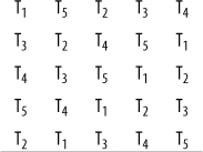
Using a Latin square in this way ensures that any between-subjects variation affects all treatments in an equal way. Note that there are 161,279 other possible randomizations of the 5×5 Latin square that would retain their characteristic property of no orthogonal (row or column) having the same number more than once. If your design required at least one instance of the ordinal presentation of treatments (T1, T2, T3, T4, and T5), the reduced form could be used—because the first row and column would preserve ordinality—but would yield only 55 possible randomizations. Latin squares for a few conditions are easily constructed by hand, but you can find a table of Latin squares online as well as a simple algorithm to construct them.
This section reviews a real example of an experiment and discusses the design decisions made, comparing how it could have been conducted using two common experimental designs, and provides examples that highlight the relative strengths and/or weaknesses of each strategy.
Frances H. Martin and David A.T. Siddle (2003; full citation is included in Appendix C) set out to investigate the main effects of alcohol and tranquilizers on reaction time, P300 amplitude and P300 latency, as well as their interaction. P300 amplitude and latency are measures derived from event-related potentials in the brain at 300ms. All three responses are related to different information-processing mechanisms in the brain.
The research question was based on previous studies that had independently demonstrated the impact of alcohol or tranquilizers on these response variables but not their interaction. In addition, studies investigating the effect of alcohol on the response variables tended to use large doses, and studies looking at tranquilizers focused on strong tranquilizers, whereas in this study, a mild tranquilizer, Temazepam, was selected. Thus, three questions were posed:
Does alcohol have a significant main effect on any of the response variables?
Does Temazepam have a significant main effect on any of the response variables?
Do alcohol and Temazepam interact?
The experiment used a within-subjects design so that participants acted as their own controls. The factorial design was 2 (alcohol, control) ×2 (tranquilizer, control); thus, every participant performed the same experiment four times with the following conditions:
No alcohol and no Temazepam
Alcohol only
Temazepam only
Both alcohol and Temazepam
The results indicated a significant main effect for Temazepam on P300 amplitude (that is, this effect was present with or without alcohol) and significant main effect for alcohol on P300 latency and reaction time. However, there was no significant interaction between the two factors. Given that alcohol and Temazepam have different main effects, and because they don’t interact, the study supports the idea that alcohol and Temazepam independently affect different information-processing mechanisms in the brain.
If you were designing this experiment, what would you have done? Would you have selected a matched-pair design instead of a within-subjects design? This would have reduced the number of trials that each participant had to complete, but in this instance, using a within-subjects design also allowed for smaller participant numbers to be used (N = 24), whereas a larger sample might have been needed to demonstrate an effect between subjects. No doubt you would have randomized the selection of participants, perhaps by selecting names from a phone book, using page numbers and columns generated by a random number generator. Content validity would not be a concern because the response variables used are widely accepted in the field as reflecting information-processing characteristics of the brain. You would also have ensured blinding of the researcher administering the alcohol or Temazepam, ensuring that the control for each was physically the same in appearance. Would you have chosen to increase the number of factors rather than having a 2×2? For example, perhaps there would only be an interaction between alcohol and Temazepam at high respective dosages, so perhaps a 3×3 design would have been more appropriate. The question here is not necessarily experimental but ethical; you want to limit the amount of tranquilizer being administered to each participant, and in the absence of a compelling theoretical reason (or clinical evidence or observation) to suspect otherwise, the choice of a 2×2 study makes sense.