Many statistical techniques used in education and psychology are common to other fields of endeavor: these include the t-test (covered in Chapter 6), various regression and ANOVA models (covered in Chapters 8 through 11), and the chi-square test (covered in Chapter 5). The discussion of measurement in Chapter 1 will also prove useful because much of educational and psychological research involves constructs that cannot be observed directly and have no obvious units of measurement. Examples of such constructs include mechanical aptitude, self-efficacy, and resistance to change. This chapter concentrates on statistical procedures used in the field of psychometrics, which is concerned with the creation, validation, and use of tests and measurements applied to human intelligence, knowledge, abilities, and psychological characteristics such as personality traits.
The first question you may ask with regard to the use of statistics in education and psychology is why they are necessary at all. After all, isn’t every person an individual, and isn’t the point of both education and psychology to perceive each person in all his individual richness, not to reduce the individual to a set of numbers or place him in comparison with others?
This is a valid concern and underscores what anyone working in the human sciences knows already: doing research on human beings is in many ways much more difficult than doing research in the hard sciences or in manufacturing because people are infinitely more varied than chemical molecules or lug nuts. The diversity and individuality of people makes research in those fields particularly difficult. It’s also true that although some educational and psychological research is aimed toward making general statements about groups of people, a great deal of it is focused on understanding and helping individuals, each of whom has her own specific social circumstances, family histories, and other contextual complexities, making direct comparisons between one person and another very difficult.
However, standard statistical procedures can be useful even in the most specific and individual therapeutic circumstances, such as when the goal of an encounter is to devise an appropriate educational plan for one student or therapeutic regimen for one patient. Making such decisions is difficult but would be even more difficult without the aid of formal educational and psychological tests that yield numeric values and can be compared to scores for other individuals. No one would suggest that only formal, standardized tests and questionnaires be used in these contexts; interviews and observational testing play an important role in educational and psychological evaluations as well. But the advantages of including formal testing procedures and standardized tests in clinical and educational evaluations include the following considerations:
Objective comparisons are facilitated by the use of a normative group. For instance, is this patient, recovering from trauma, experiencing more side effects than is common among others who have experienced the same injury? Are the reading skills of this pupil comparable to others of his age and grade level?
Standardized testing can yield results quickly; you needn’t wait for the end of the school term to discover which pupils are struggling because of poor language proficiency, and you don’t need a lengthy interview or practical examination to discover that a patient is suffering from serious memory deficits.
Standardized tests are presented in a regulated situation and under specified conditions and can be scored objectively, so the only issue being evaluated is the student’s or patient’s performance, not her appearance, sociability (unless that is germane to the context), or other irrelevant factors.
Most standardized tests do not require great skill to administer (unlike clinical interviews, for example) and can be given to groups of people at once, making the tests particularly useful as screening procedures.
In many countries, school-age children are evaluated by tests that report their results in percentiles, also known as percentile ranks; one student might score in the 70th percentile in reading and the 85th percentile in math, but another scores in the 80th percentile in reading and the 95th percentile in math. Percentiles are a form of norm-referenced scoring, so called because an individual score is placed in the context of a norm group, meaning people similar to the test-taker. For school-age children, the norm group is often other children in the same grade within their country. Norm-referenced scoring is used in all kinds of testing situations in which an individual’s rank in relation to some comparison group is more important than his absolute score.
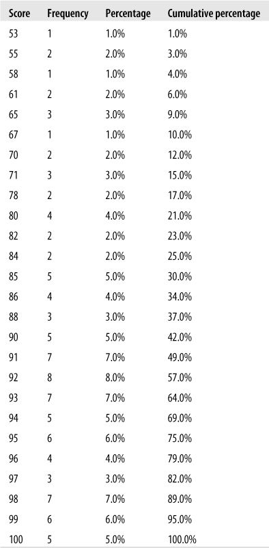
The percentile rank of an individual score refers to the percentage in the norm group that scored lower than that individual score, so a percentile score of 90 indicates that 90% of the norm group scored lower. Here’s a brief example illustrating how to find percentile ranks for scores on an exam that was given to 100 students. (On national exams, the norm group would be much larger and the scores would reflect a greater range, but this example will illustrate the point.)
The first step in translating from raw scores to percentiles is to create a frequency table that includes a column for cumulative percentage, as illustrated in Figure 16-1. To find the percentile rank for a particular score, use the cumulative percentage from the next-highest score, the row just above in the table. In this example, someone who scored 96 on the exam was in the 75th percentile rank (meaning 75% of the test-takers scored below 96), whereas someone who scored 85 was in the 25th percentile rank. There can be no 100th percentile rank because, logically speaking, 100% of the test-takers couldn’t have scored below a score that is included in the table. You can have a 0th percentile, however; a person who scored 53 would be in the 0th percentile because no one achieved a lower score.
In situations such as standardized testing at the national level, the norm group used to map the scores to percentiles is much larger, and generally, calculation of percentiles for individual students is not necessary. Instead, the test manufacturer usually provides a chart that relates raw scores to percentile ranks.
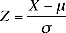
The standardized score, also known as the normal score or the Z-score, transforms a raw score into units of standard deviation above or below the mean. This translates the scores so they can be evaluated in reference to the standard normal distribution, which is discussed in detail in Chapter 3. Standardized scores are frequently used in education and psychology because they place a score in the context of other scores and can therefore be considered a type of norm-referenced scoring. For frequently used scales such as the Wechsler Adult Intelligence Scale (WAIS), population means and standard deviations are known and may be used in the calculations; for the WAIS, the mean is 100, and the standard deviation is 15. To convert a raw score to a standardized score, use the formula shown in Figure 16-2.
| In this formula, X is the raw score, |
| µ is the population mean, |
| and σ is the population standard deviation. |
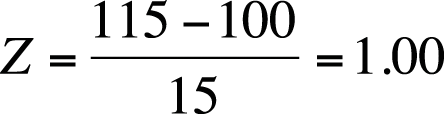
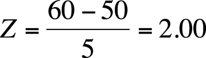
The conversion to Z-scores puts all scores on a common scale, that of the standard normal distribution with a mean of 0 and a variance of 1. In addition, Z-score probabilities are distributed with the known properties of the normal distribution. (For instance, about 66% of the scores will be within one standard deviation of the mean.) We can convert a raw score of 115 on the WAIS to a Z-score as shown in Figure 16-3.
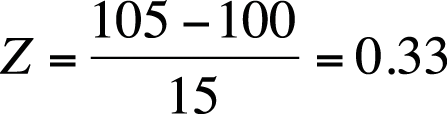
Using the table for the standard normal distribution (Z distribution) in Figure D-3 from Appendix D, we see that a Z-score of 1.00 means that 84.1% of individuals score at or below that individual’s raw score. Standardized scores are particularly useful when comparing scores on tests with different scales. For example, let’s say we also administer a test of mathematical aptitude that has a mean of 50 and a standard deviation of 5. If a person scores 105 on the WAIS (Figure 16-4) and 60 on the mechanical aptitude (Figure 16-5), we can easily compare those scores in terms of Z-scores.
The Z-scores tell us that this person scored slightly above average in intelligence but far above average in mechanical aptitude.
Some people find standardized scores confusing, particularly because a person can have a Z-score that is 0 or negative (and in the standard normal distribution, half the scores are below average and therefore negative). For this reason, Z-scores are sometimes converted to T-scores, which use a more intuitive scale, with a mean of 50 and a standard deviation of 10. Z-scores may be converted to T-scores by using the following formula:
If a person has a Z-score of 2.0 (meaning he or she scored two standard deviations above the mean), this can be converted to a T-score as follows:
Similarly, someone with a Z-score of −2.0 would have a T-score of 30. Because hardly anyone ever scores five standard deviations or more below the mean, T-scores are almost always positive, which makes them easier for many people to understand. For instance, the clinical scales of the Minnesota Multiphase Personality Inventory-II (MMPI-II), commonly used to identify and evaluate psychiatric conditions, are reported as T-scores.
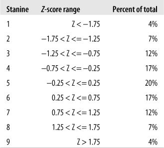
Stanines offer another method to translate raw scores into scores based on the standard normal distribution. The term “stanine” is an abbreviation of “standard nine” and refers to the fact that stanines divide scores into nine categories (1−9), each category or band representing half a standard deviation of the standard normal distribution. The mean of the stanine scale is 5, and this category includes scores that translate to standard scores from −0.25 to 0.25 (one quarter of a standard deviation below or above the mean). The primary advantage of using stanines instead of Z- or T-scores is that reporting categories rather than specific scores might get around the human tendency to obsess over small differences in reported scores.
Because scores near the central value of the normal distribution are more common than extreme scores, stanines near the central value of 5 are more common than scores near the extremes of 1 or 9. Note also that the distribution of stanine scores is symmetrical, as is the distribution of scores in the standard normal distribution, so a stanine of 1 is as common as a stanine of 9, a stanine of 2 is as common as a stanine of 8, and so on. The application of these two principles can be seen in Figure 16-6, which shows the stanine score, the corresponding standard (Z) scores, and the percentage of the distribution contained within each stanine category.
Stanines may be calculated from Z-scores by using the following formula:
Stanines are rounded to the nearest whole number; values with a decimal of 0.5 are rounded down. Suppose we have a Z-score of −1.60. This translates to a stanine of 2, as shown below:
The nearest whole number is 2, and this corresponds to the stanine value for a Z-score of −1.60 given in Figure 16-6.
A Z-score of 1.60 translates to a stanine of 8 because:
The nearest whole number is 8, and this stanine value corresponds with the value indicated in Figure 16-6 for a Z-score of 1.60.
Most tests in psychology and education are used for what is called subject-centered measurement, in which the purpose is to place individuals on a continuum with respect to particular characteristics such as language-learning ability or anxiety. Creating and validating a test is a huge amount of work. (When I was in graduate school, students were barred from writing a dissertation that required creating and validating a new test out of fear that they would never complete the process.) The burden is entirely on the test’s creator to convince others working in the same field that the test scores are meaningful. Therefore, the first move for someone beginning to investigate a field is to check whether any existing, validated tests would be adequate. However, particularly if you are researching a new topic or dealing with a previously ignored population, no existing test might be adequate to your purpose, in which case the only option is to create and validate a new test.
Tests can be either norm-referenced or criterion-referenced. Norm-referenced tests have already been discussed; their purpose is to place an individual in the context of some group. In contrast, the purpose of a criterion-referenced test is to compare an individual to some absolute standard, say, to see whether he has obtained a defined minimum competency in an academic subject. In a criterion-referenced test, everyone taking the test could receive a high score, or everyone could receive a low score, because the individuals are evaluated with reference to a predetermined standard rather than in reference to each other. Although criterion-referenced tests can yield a continuous outcome (for instance, a score on a scale of 1−100), a cut point (single score) is often established as well so that everyone who achieves that score or above passes, and everyone with a score below it fails.
Most tests are composed of numerous individual items, often written questions, which are combined (often simply added together) to produce a composite test score. For instance, a test of language ability might be constructed of 100 items with each correct item scored as a 1 and each incorrect item as a 0. The composite score for an individual could then be determined by adding up the number of correct items. Many of the statistical procedures used in examining tests have to do with the relationship among individual items and the relation between individual items and the composite score.
Although composite test scores are commonly used, they can be misleading measures of ability or achievement. One difficulty is that typically all items are assigned the same weight toward the total score, although they might not all be of equal difficulty. The distinction between someone who misses some easy questions but gets more difficult questions correct versus someone who gets the easy questions correct but can’t answer the difficult questions is lost when a composite score is formed by simply summing the scores of items of differing homogeneity.
The mean and variance of dichotomous items (those scored as either right or wrong) are calculated using the value for item difficulty, signified as p. Item difficulty is the proportion of examinees who answer a question correctly. If N people are in the group of examinees used to establish item difficulty, p is calculated for one item (j) as shown in Figure 16-7.

With dichotomous items scored 0 or 1 (0 for incorrect, 1 for correct), the mean is the same as the proportion answering the item correctly (Figure 16-8).
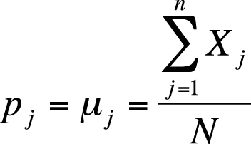
| In this formula, Xj are the individual items, |
| and N is the number of examinees |
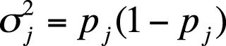
Variance for an individual dichotomous item pj may be calculated as shown in Figure 16-9.
The correlation coefficient between two dichotomous items, also called the phi coefficient, is discussed in Chapter 5.
Computing the variance of a composite score requires knowing both the individual item variances and their covariances. Unless all pairs of variables are completely uncorrelated or are negatively correlated, the variance of a composite score will always be greater than the sum of the individual item variances. Although composite variance is usually computed using statistical software, the formula is useful to know because it outlines the relationship among the relevant quantities. The covariance for a pair of items j and k (whether the items are dichotomous or continuous) may be computed as shown in Figure 16-10.

| In this formula, σjk is the covariance of the two items, |
| ρjk is the correlation between the two items, |
| and σj and σk are the individual item variances. |
Often, we are interested in the variance of a composite such as a test score Y consisting of numerous items. Because there are two covariance pairs for each item pair (the covariance of j with k, and the covariance of k with j, which are identical), the covariance of a composite Y may be calculated as shown in Figure 16-11.
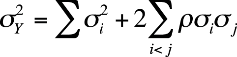
The stipulation i < j in the preceding formula stipulates that we compute only unique covariance terms. To get the right number of covariance terms, we then multiply each unique covariance by 2.
As items are added to a test, the number of covariance terms increases more quickly than the number of variance terms. For instance, if we add 5 items to a test that has 5 items to start with, the number of variance terms increases from 5 to 10, but the number of covariance items increases from 20 to 90. The number of unique covariance terms for n items is calculated as n(n − 1); therefore, a test with 5 items has 5(4) = 20 covariance terms. A 10-item test would have 10(9) = 90 covariance terms. The number of unique covariance terms is [n (n − 1)]/2, so 5 items yield 10 unique covariance terms, and 10 items yield 45 unique covariance terms.
In most cases, adding items to a composite increases the variance of the composite because the variance of the composite is increased by the variance of the individual item plus its covariance with all the existing items on the test. The proportional increase is greater when items are added to a short test than to a long test and is greatest when items are highly correlated because that results in larger covariances among items. All else being equal, the greatest composite variance is produced by items of medium difficulty (p = 0.5 produces the largest covariance scores) that are highly correlated with one another.
In an ideal world, all tests would have perfect reliability, meaning that if the same individuals were tested repeatedly under the same conditions for some stable characteristic, they would receive identical scores each time, and there would be no systematic error (defined later) in the score. In this case, we would have no problem saying that a person’s observed score on the test was the same as the person’s true score and that the observed score was an accurate reflection of that person’s score on whatever the test was designed to measure. In the real world, however, many factors can influence observed scores, and repeated tests on the same material taken by the same individual often yield different scores. For this reason, we must differentiate between the true score and the observed score. We do this by introducing the concept of measurement error, which is the part of the observed score that causes it to deviate from the true score.
Measurement error can be either random or systematic. Random measurement error is the result of chance circumstances such as room temperature, variance in administrative procedure, or fluctuation in the individual’s mood or alertness. We do not expect random error to affect an individual’s score consistently in one direction or the other. Random error makes measurement less precise but does not systematically bias results because it can be expected to have a positive effect on one occasion and a negative effect on another, thus canceling itself out over the long run. Because there are so many potential sources for random error, we have no expectation that it can be completely eliminated, but we desire to reduce it as much as possible to increase the precision of our measurements. Systematic measurement error, on the other hand, is error that consistently affects an individual’s score in one direction but has nothing to do with the construct being tested. An example would be measurement error on a mathematics exam that is caused by poor language skills so that the examinee cannot read the directions to take the exam properly. Systematic measurement error is a source of bias and should be eliminated from testing whenever possible.
The psychologist Charles Spearman introduced the classic concepts of true and error scores in the early twentieth century. Spearman described the observed score X (the score actually received by an individual on a testing occasion), which is composed of a true component (T) and a random error component (E):
Over an infinite number of testing occasions, the random error component is assumed to cancel itself out, so the mean or expected value of the observed scores is the same as the true score. For individual j, this can be written as:
where Tj is the true score for individual j, E(Xj) is that individual’s expected observed score over an infinite number of testing occasions, and µXj is the mean observed score for that individual over the same occasions. Error is therefore the difference between an individual’s observed score and her true score:
Over an infinite number of testing occasions, the expected value of the error for one individual is 0. Because “error” in this definition means random error only, true and error scores are assumed to have the following properties:
Over a population of examinees, the mean of the error scores is 0.
Over a population of examinees, the correlation between true and error scores is 0.
The correlation between error scores by two randomly chosen examinees on two forms of the same test, or two testing occasions using the same form, is 0.
When we administer a test to an individual, one of our concerns is how well the observed score on that test represents the person’s true score. In theoretical terms, what we seek is the reliability index for the test, which is the ratio of the standard deviation of the true scores to the standard deviation of the observed scores. The reliability index is calculated as shown in Figure 16-12.
| In this formula, σT is the standard deviation of the true scores for a population of examinees, |
| and σX is the standard deviation of their observed scores. |
The reliability of a test is sometimes described as the proportion of total variation on the test scores that is explained by true variation (as opposed to error).
In practice, true scores are unknown, so the reliability index must be estimated using observed scores. One way to do this is to administer two parallel tests to the same group of examinees and use the correlation between their scores on the two forms, known as the reliability coefficient, as an estimate of the reliability index. Parallel tests must satisfy two conditions: equal difficulty and equal variance.
The reliability coefficient is an estimate of the ratio of true score variance to observed score variance and can be interpreted similarly to the coefficient of determination (r2) in the general linear model. If a test reports a reliability coefficient of 0.88, we can interpret this as meaning that 88% of the observed score variance from administrations of this test is due to true score variance, whereas the remaining 0.12 or 12% is due to random error. To find the correlation between true and observed scores for this test, we take the square root of the reliability coefficient, so for this test, the correlation between true and observed scores is estimated as √0.88, or 0.938.
The reliability coefficient can be estimated using one of several methods. If we estimate the reliability coefficient by administering the same test to the same examinees on two occasions, this is called the test-retest method, and the correlation between test scores in this case is known as the coefficient of stability. We could also estimate the reliability coefficient by administering two equivalent forms of a test to the same examinees on the same occasion; this is the alternate form method, and the correlation between scores is the coefficient of equivalence. If both different forms and different occasions of testing are used, correlation between the scores under these conditions is called the coefficient of stability and equivalence. Because this coefficient has two sources of error, forms and occasions, it is generally expected to be lower than either the coefficient of stability or the coefficient of equivalence would be for a given group of examinees.
A different approach to estimating reliability is to use a measure of internal consistency that can be calculated from a single administration of a test to a single group of examinees. Consistency measurements are used to estimate reliability because a composite test is often conceived of as being composed of test items sampled from a large domain of potential items. An internal consistency estimate is a prediction of how similar an individual’s score would be if a different subset of items from that domain had been chosen.
Consider the task of creating an exam to test student competence in high school algebra. The first steps in creating this test would be to decide what topics to cover. Then a pool of items would be written that evaluate student mastery of those topics. A subset of items would then be chosen to create the final test. The purpose of this type of exam is not merely to see how well the students score on the specific items included in the test they took but how well they mastered all the content considered to be within the domain of high school algebra. If the items used on the test are a fair selection from this content domain, the test score should be a reliable indicator of the students’ mastery of the material. Item homogeneity is also a valued characteristic of this type of test because it is an indication that the items are testing the same content and do not have technical flaws such as misleading wording or incorrect scoring that would cause performance on an item to be unrelated to mastery of algebra.
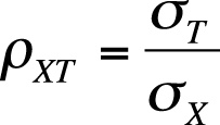
Split-half methods to measure internal consistency require a test to be split into two parts or forms, usually two halves of equal length, which are intended to be parallel. All items on the full-length test are completed by each examinee. The split can be achieved by several methods, including alternate assignment (even-numbered items to one form, odd-numbered to the other), content matching, or random assignment. Whichever method is used, if the original test had 100 items, the two halves will each have 50 items. The correlation coefficient between examinee scores for the two forms is called the coefficient of equivalence. The coefficient of equivalence is an underestimate of the reliability for the full-length test because longer tests are usually more reliable than shorter tests. The Spearman-Brown prophecy formula can be used to estimate the reliability of the full-length test from the coefficient of equivalence for the two halves, using the formula shown in Figure 16-13.
| In this formula, ρXX’ is the estimated reliability of the full-length test, |
| and ρAB is the observed correlation, that is, coefficient of equivalence, between the two half-tests. |
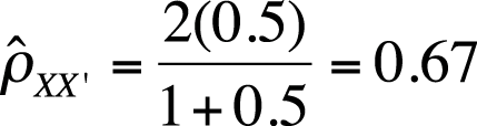
For this formula to be accurate, the two half-tests must be strictly parallel. If the coefficient of equivalence for the two half-tests is 0.5, the estimated reliability of the full-length test is shown in Figure 16-14.
A second method to estimate reliability of a full-length test using the split-half method is to calculate the difference between scores on the two halves for each examinee. The variance of that difference score is an estimate of error variance of reliability, so the 1 minus the ratio of error variance to total variance may also be used as an estimate of reliability. Figure 16-15 presents the formula to use for the second method.
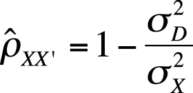
| In this formula, σ2D is the variance of the difference scores, |
| and σ2X is the variance of the observed scores. |
Estimates of reliability using either method will be identical when the variance of the two half-tests is identical. The more dissimilar the two variances, the larger the estimate using the Spearman-Brown formula will be relative to estimates using the difference-score method. Estimation of reliability by either method depends on how the items are chosen for the two halves because a different split will result in different correlations between the halves and a different set of difference scores.
Several methods of estimating reliability using item covariances avoid the problem of multiple split-half reliabilities; three of these methods follow. Cronbach’s alpha may be used for either dichotomous or continuously scored items, whereas the two Kuder-Richardson formulas are used only for dichotomous items. The measure of internal consistency computed by any of these methods is commonly referred to as coefficient alpha and is equivalent to the mean of all possible split-half coefficients computed using the difference-score method. Coefficient alpha is, strictly speaking, not an estimate of the reliability coefficient but of its lower bound (sometimes called the coefficient of precision). This nicety is often ignored in interpretation, however, and coefficient alpha is usually reported without further interpretation.
Note that computing coefficient alpha for a test of any considerable length is tedious and therefore generally accomplished using computer software. Still, it is useful to know the formulas and work through a simple calculation to understand what factors affect coefficient alpha.
Cronbach’s alpha is the most common method for calculating coefficient alpha and is the name often given for coefficient alpha in computer software packages designed for reliability analysis. It is computed using the formula shown in Figure 16-16.
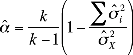
| In this formula, k is the number of items, |
 is the variance of item i, and is the variance of item i, and |
 is the total test variance. is the total test variance. |
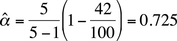
Suppose we have a 5-item test, with a total test variance of 100 and individual item variances of 10, 5, 6.5, 7.5, and 13. Cronbach’s alpha for this data set is shown in Figure 16-17.
There are several Kuder-Richardson formulas to calculate coefficient alpha; two useful for dichotomous items are presented here. Note that KR-21 is a simplified version of the KR-20 formula; it assumes all items are of equal difficulty. KR-20 and KR-21 yield identical results if all items are of equal difficulty; if they are not, KR-21 yields lower results than KR-20. The KR-20 formula is shown in Figure 16-18.
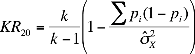
| In this formula, k is the number of items, |
| pi is the difficulty for a given item, and |
| is the total variance. |
Note that the KR-20 formula is identical to the Cronbach’s alpha formula with the exception that the item variance term has been restated to take advantage of the fact that KR-20 is used for dichotomous items.
The KR 20 formula can be simplified by assuming all items have equal difficulty, so it is not necessary to compute and sum the individual item variances. This simplification yields the KR 21 formula (Figure 16-19).
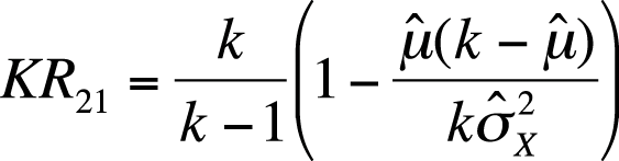
| In this formula, k is the number of items, |
 is the overall mean for the test (usually estimated by is the overall mean for the test (usually estimated by  ), and ), and |
| is the total variance for the test (usually estimated by s2x. |
Test construction often proceeds by creating a large pool of items, pilot-testing them on examinees similar to those for whom the test is intended, and selecting a subset for the final test that makes the greatest contributions to test validity and reliability. Item analysis is a set of procedures used to examine and describe examinees’ responses to the items under consideration, including the distribution of responses to each item and the relationship between responses to each item and other criteria.
One of the first things usually computed in an item analysis is the mean and variance of each item. For dichotomous items, the mean is also the proportion of examinees who answered the item correctly and is called the item difficulty or p, as previously discussed. The total test score for one examinee is the sum of the item difficulties, which is the same as the sum of questions answered correctly. The average item difficulty is the sum of the item difficulties divided by the number of items, as shown in Figure 16-20.
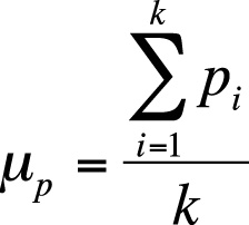
| In this formula pi is the difficulty of item i, |
| and k is the total number of items. |
Because item difficulty is a proportion, the variance for an individual item is:
Often, items are selected to maximize variance to increase the test’s efficiency in discriminating among individuals of different abilities. Variance is maximized when p = 0.5, a fact that you can confirm for yourself by calculating the variance for some other values of p:
| If p = 0.50, σ2i = 0.5(0.5) = 0.2500 |
| If p = 0.49, σ2i = 0.49(0.51) = 0.2499 |
| If p = 0.48, σ2i = 0.48(0.52) = 0.2496 |
| If p = 0.40, σ2i = 0.40(0.60) = 0.2400 |
Note that the variances for p = 0.49 and p = 0.51 are identical, as are the variances for p = 0.48 and p = 0.52, and so on.
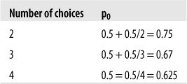
In many common test formats, most obviously multiple choice, examinees might raise their scores by guessing if they don’t know the correct answer. This means that the p value of an item will often be higher than the proportion of examinees who actually know the material tested by the item. To put it another way, the observed scores will be systematically higher than the true scores because the observed scores have been raised by successful guessing. For this reason, when an item format allows guessing (for instance, with multiple choice items that carry no penalty for incorrect answers), an additional step is necessary to calculate the observed difficulty of an item to maximize item variance. This is done by adding the quantity 0.5/m to the item difficulty, where m is the number of choices for an item. This formula assumes that the choices are equally likely to be selected if the examinee doesn’t know the correct answer to the item. The observed difficulty p0 of an item that is assumed to have a true difficulty of 0.5 (half the examinees know the correct answer without guessing) for different values of m would be as shown in Figure 16-21.
Item discrimination refers to how well an item differentiates between examinees with high versus low amounts of the quality being tested, whether it is knowledge of geography, musical aptitude, or depression. Normally, the test creator selects items that have positive discrimination, meaning they have a high probability of being answered correctly or positively by those who have a large amount of the quality, and incorrectly or negatively by those who have a small amount. For instance, if you are measuring mathematical aptitude, questions with positive discrimination are much more likely to be answered correctly by students with high mathematical aptitude as opposed to those with low mathematical aptitude, who are unlikely to answer correctly. The reverse quality is negative discrimination; continuing with this example, an item with negative discrimination would be more likely to be answered correctly by a student with low aptitude than a student with high aptitude. Negative discrimination is usually grounds to eliminate an item from the pool unless it is being retained to catch people who are faking their answers (for instance, on a mental health inventory).
Four indices of item discrimination are discussed in this section, followed by an index of item discrimination that can be related either to total test score or to an external criterion. If all items are of moderate difficulty (which is typical of many testing situations), all five discrimination indices will produce similar results.
The index of discrimination is only applicable to dichotomously scored items; it compares the proportion of examinees in two groups that answered the item correctly. The two groups are often formed by examinee scores on the entire test; for instance, the upper 50% of examinees is often compared to the lower 50% or the upper 30% to the lower 30%. The formula to calculate the index of discrimination (D) is:
| where pu is the proportion in the upper group that got the item correct, and |
| pl is the proportion in the lower group that got it correct. |
If 80% of the examinees in the upper group got an item correct, but only 30% of those in the lower group got it correct, the index of discrimination would be:
The range of D is (−1, +1). D = 1.0 would mean that everyone in the upper group got the item correct and no one in the lower group did, so the item achieved perfect discrimination; D = 0 would mean that the same proportion in the upper and lower groups got the item correct, so the item did not discriminate between them at all. The index of discrimination is affected by how the upper and lower groups are formed; for instance, if the upper group were the top 20% and the lower group the bottom 20%, we would expect to find a larger index of discrimination than if the upper 50% and lower 50% were used.
There are no significance tests for the index of discrimination and no absolute rules about what constitutes an acceptable value. A rule of thumb suggested by Ebel (1965; full citation in Appendix C) is that D > 0.4 is satisfactory (items can be used), D < 0.2 is unsatisfactory (items can be discarded), and the range between suggests that the items should be revised to raise D above 0.4.
The point-biserial correlation coefficient, discussed in Chapter 5, is a measure of association between a dichotomous and a continuous variable; it may be used to measure the correlation between a single dichotomous item and the total test score (assuming the test contains enough items that the scores are continuous).
The biserial correlation coefficient may be calculated for dichotomous items if it is assumed that performance on the item is due to a latent quality that is normally distributed. The formula to calculate the biserial correlation coefficient is given in Figure 16-22.
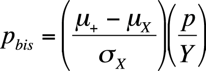
| In this formula, µ+ is the average total test score for examinees who answered the item correctly, |
| µX is the average total score for the entire examinee group, |
| σX is the standard deviation on the total score for the entire group, |
| p is the item difficulty, and |
| Y is the Y-coordinate (height of the curve) from the standard normal distribution for the item difficulty (e.g., from Figure D-3 in Appendix D). |
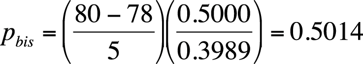
Suppose for a given item, µ+ = 80, µX = 78, σX = 5, and p = 0.5. The biserial correlation coefficient for this item is shown in Figure 16-23.
The value of the biserial correlation is systematically higher than the point-biserial correlation for the same data, and the difference increases sharply if p < 0.25 or p > 0.75. The biserial correlation coefficient is the preferred item difficulty statistic when a dichotomous item is assumed to reflect an underlying normal distribution, and the goal is to select items that are very easy or very difficult or if the test will be used with future groups of examinees with a wide range of ability.
The phi coefficient, discussed in Chapter 5, expresses the relationship between two dichotomous variables. If the variables are not true dichotomies but have been created by dichotomizing values from a continuous variable with an underlying normal distribution (such as a pass/fail score determined by establishing a single cut point for a continuous variable), the tetrachoric correlation coefficient is preferred over the phi coefficient because the range of phi is restricted when the item difficulties are not equal. Tetrachoric correlations are also used in factor analysis and structural equation modeling. The tetrachoric correlation coefficient is rarely computed by hand but is included in some of the standard statistical software packages, including SAS and R.
Although analyses based on classical test theory are still used in many fields, item response theory (IRT) offers an important alternative approach. Anyone working in psychometrics should be aware of IRT, and it is being used increasingly in other fields, from medicine to criminology. IRT will probably be used even more in the future because IRT capabilities are implemented into commonly used statistical packages. IRT is a complex topic and can be only briefly introduced here; those who wish to pursue it should consult a textbook such as Hambleton, Swaminathan, and Rogers (1991) or a similar introductory textbook. An inventory of computer packages for IRT is available from the Rasch SIG.
IRT addresses several failings of classic test theory chief among them is the fact that methods based on classic test theory cannot separate examinee characteristics from test characteristics. In classic theory, an examinee’s ability is defined in terms of a particular test, and the difficulty of a particular test is defined in terms of a particular group of examinees. This is because the difficulty of a test item is defined in classic theory as the proportion of examinees getting it correct; with one group of examinees, an item might be classified as difficult because few got it correct, whereas for another group of examinees, it might be classified as easy because most got it correct. Similarly, on one test, an examinee might be rated as having high ability or having mastered a body of material because she got a high score on the test, whereas on another test ostensibly covering the same basic material, she might be rated as having low ability or mastery because she got a low score.
The fact that estimates of item difficulty and examinee ability are intertwined in classic test theory means that it is difficult to make an equivalent estimation of ability comparing examinees who take different tests or to rate the difficulty of items administered to different groups of examinees. Classic test theory has tried various procedures to deal with these issues, such as including a common body of items on different forms of a test, but the central problem remains:
Performance of a given examinee on a given item can be explained by the examinee’s ability on whatever the item is testing, and ability is considered to be a latent, unobservable trait.
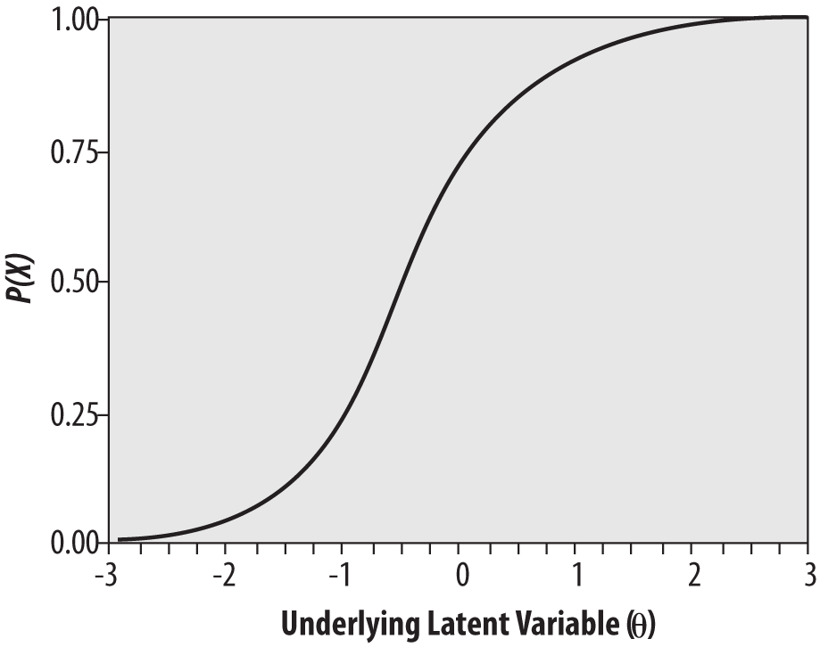
An item characteristic curve (ICC) can be drawn to express the relationship between the performance of a group of examinees on a given item and their ability.
Ability is usually represented by the Greek letter theta (θ), whereas item difficulty is expressed as a number from 0.0 to 1.00. The ICC is drawn as a smooth curve on a graph in which the vertical axis represents the probability of answering an item correctly, and the horizontal axis represents examinee ability on a scale in which θ has a mean of 0 and a standard deviation of 1. The ICC is a monotonically increasing function, so that examinees with higher ability (those with a higher value of θ) will always be predicted to have a higher probability of answering a given item correctly. This is shown in the theoretical ICC shown in Figure 16-24.
IRT models, in relation to classic test theory models, have the following advantages:
IRT models are falsifiable; the fit of an IRT model can be evaluated and a determination made as to whether a particular model is appropriate for a particular set of data.
Estimates of examinee ability are not test-dependent; they are made in a common metric that allows comparison of examinees who took different tests.
Estimates of item difficulty are not examinee-dependent; item difficulty is expressed in a common metric that allows comparison of items administered to different groups.
IRT provides individual estimates of standard errors for examinees rather than assuming (as in classic test theory) that all examinees have the same standard error of measurement.
IRT takes item difficulty into account when estimating examinee ability, so two people with the same number of items correct on a test could have different estimates of ability if one answered more difficult questions correctly than did the other.
One consequence of points 2 and 3 is that in IRT, estimates of examinee ability and item difficulty are invariant. This means that, apart from measurement error, any two examinees with the same ability have the same probability of answering a given item correctly, and any two items of comparable difficulty have the same probability of being answered correctly by any examinee.
Note that although in this discussion we assume items are scored as right or wrong (hence, language such as “the probability of answering the item correctly”), IRT models can also be applied in contexts in which there is no right or wrong answer. For instance, in a psychological questionnaire measuring attitudes, the meaning of item difficulty could be described as “the probability of endorsing an item” and θ as the degree or amount of the quality being measured (such as favorable attitude toward civic expansion).
Several models are commonly used in IRT that differ according to the item characteristics they incorporate. Two assumptions are common to all IRT models.
- Unidimensionality
Items on a test measure only one ability; this is defined in practice by the requirement that performance on test items must be explicable with reference to one dominant factor.
- Local independence
If examinee ability is held constant, there is no relationship between examinee responses to different items; that is, responses to the items are independent.
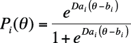
The simplest IRT model includes only one characteristic of the item, item difficulty, signified by bi. This is the one-parameter logistic model, also called the Rasch model because it was developed by the Danish mathematician Georg Rasch. The ICC for the one-parameter logistic model is computed using:
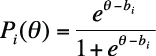
| where Pi (θ) is the probability that an examinee with ability θ will answer item i correctly, |
| and bi is the difficulty parameter for item i. |
Item difficulty is defined as the point on the ability scale (x-axis) where the probability of an examinee getting the item correct is 0.5. For more-difficult items, greater examinee ability is required before half the examinees are predicted to get it right, whereas for easier items, a lower level of ability is required to reach that point. In the Rasch model, the ICCs for items of differing difficulties have the same shape and differ only in location. This is apparent in Figure 16-25, which displays ICCs for several items of equal discrimination that vary in difficulty.
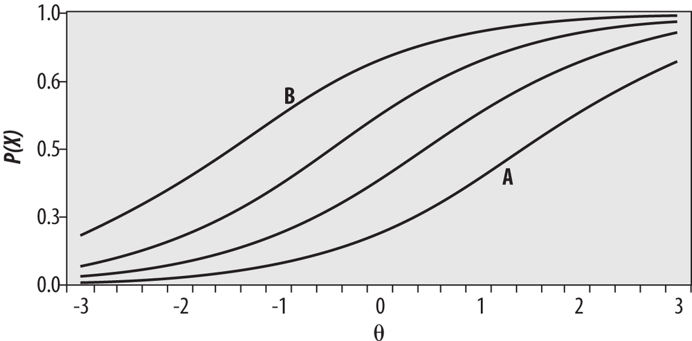
Bearing in mind that θ is a measure of examinee ability, one can see that a greater amount of ability is required to have a 50% probability of answering item A correctly compared with items further to the left. It is also clear that among the items graphed here, the least amount of θ is required to have a 50% chance of answering item B correctly. Therefore, we would say that item B is the easiest among these items and item A the most difficult. You can demonstrate this to yourself by drawing a horizontal line across the graph at y = 0.5 and then a vertical line down to the x-axis where the horizontal line intersects each curve. The point where each vertical line intersects the x-axis is the amount of θ required to have a 50% probability of answering the item correctly, and this quantity is clearly larger for item A than for item B.
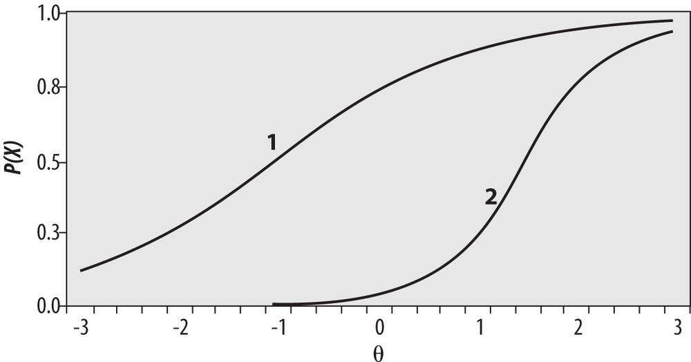
The two-parameter IRT model includes an item discrimination factor, ai. The item discrimination factor allows items to have different slopes. Items with steeper slopes are more effective in differentiating among examinees of similar abilities than are items with flatter slopes because the probability of success on an item changes more rapidly relative to changes in examinee ability.
Item difficulty is proportional to the slope at the point where bi = 0.5, that is, where half the examinees would be expected to get the item correct. The usual range for ai is (0, 2) because items with negative discrimination (those that an examinee with less ability has a greater probability to answer correctly) are usually discarded and because, in practice, item discrimination is rarely greater than 2. The two-parameter logistic model also includes a scaling parameter, D, which is added to make the logistic function as close as possible to the cumulative normal distribution.
The ICC for a two-level logistic model is computed using the following formula:
Two items that differ in both difficulty and discrimination are illustrated in Figure 16-26.
The three-level logistic model includes an additional parameter, ci, which is technically called the pseudo-chance-level parameter. This parameter provides a lower asymptote for the ICC that represents the probability of examinees with low ability answering the item correctly by chance. This parameter is often called the guessing parameter because one way low-ability applicants could get a difficult question correct is by guessing the right answer. However, often ci is lower than would be expected by random guessing because of the skill of test examiners in devising wrong answers that can seem correct to an examinee of low ability. The ICC for the three-parameter logistic model is calculated using this formula:
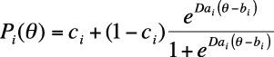
A three-parameter model is shown in Figure 16-27; it has a substantial guessing parameter, which can be seen from the fact that the curve intersects the x-axis around 0.20. This means that a person with very low θ would still have about a 20% chance of answering this item correctly.
Here is a set of questions to review the topics covered in this chapter.
Problem
Given the data distribution in Figure 16-1:
What is the percentile rank for a score of 80?
What score corresponds to a score at the 75th percentile?
Solution
You find the percentile by looking at the cumulative probability for the score just above the score you are interested in. To find a score corresponding to a percentile rank, reverse the process.
A score of 80 is in the 17th percentile.
A score of 96 is in the 75th percentile.
Problem
Assume you are working with a published test whose mean is 100 and whose variance is 400. Convert the following individual scores to Z-scores, T-scores, and stanines.
70
105
Solution
For 70, Z = −1.5, T = 35, and stanine = 2.
For 105, Z = 0.25, T = 52.5, and stanine = 5.
The computations for a score of 70 are shown in Figure 16-28 and below.
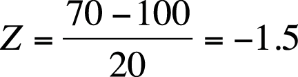
| T = −1.5(10) + 50 = 35 |
| Stanine = 2(−1.5) + 5 = 2.0 |
The computations for a score of 105 are shown in Figure 16-29 and below.
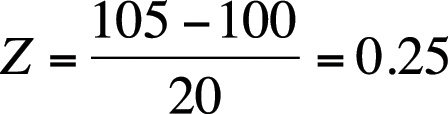
| T = 0.25(10) + 50 = 52.5 |
| Stanine = 0.25(2) + 5 = 5.5; rounds down to 5. |