3D MODELS
6.1Procedural Models – Building a Sphere
6.2OpenGL Indexing – Building a Torus
6.3Loading Externally Produced Models
So far we have dealt only with very simple 3D objects, such as cubes and pyramids. These objects are so simple that we have been able to explicitly list all of the vertex information in our source code and place it directly into buffers.
However, most interesting 3D scenes include objects that are too complex to continue building them as we have, by hand. In this chapter, we will explore more complex object models, how to build them, and how to load them into our scenes.
3D modeling is itself an extensive field, and our coverage here will necessarily be very limited. We will focus on the following two topics:
•building models procedurally
•loading models produced externally
While this only scratches the surface of the rich field of 3D modeling, it will give us the capability to include a wide variety of complex and realistically detailed objects in our scenes.
6.1PROCEDURAL MODELS – BUILDING A SPHERE
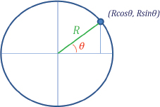
Some types of objects, such as spheres, cones, and so forth, have mathematical definitions that lend themselves to algorithmic generation. Consider for example a circle of radius R—coordinates of points around its perimeter are well defined (Figure 6.1).
Figure 6.1
Points on a circle.
We can systematically use our knowledge of the geometry of a circle to algorithmically build a sphere model. Our strategy is as follows:
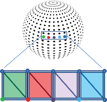
1.Select a precision representing a number of circular “horizontal slices” through the sphere. See the left side of Figure 6.2.
2.Subdivide the circumference of each circular slice into some number of points. See the right side of Figure 6.2. More points and horizontal slices produces a more accurate and smoother model of the sphere. In our model, each slice will have the same number of points.
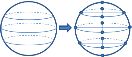
Figure 6.2
Building circle vertices.
3.Group the vertices into triangles. One approach is to step through the vertices, building two triangles at each step. For example, as we move along the row of the five colored vertices on the sphere in Figure 6.3, for each of those five vertices we build the two triangles shown in the corresponding color (the steps are described in greater detail below).
Figure 6.3
Grouping vertices into triangles.
4.Select texture coordinates depending on the nature of our texture images. In the case of a sphere, there exist many topographical texture images, such as the one shown in Figure 6.4 [VE16] for planet Earth. If we assume this sort of texture image, then by imagining the image “wrapped” around the sphere as shown in Figure 6.5, we can assign texture coordinates to each vertex according to the resulting corresponding positions of the texels in the image.

Figure 6.4
Topographical texture image [VE16].

Figure 6.5
Sphere texture coordinates.
5.It is also often desirable to generate normal vectors—vectors that are perpendicular to the model’s surface—for each vertex. We will use them soon, in Chapter 7, for lighting.
Determining normal vectors can be tricky, but in the case of a sphere, the vector pointing from the center of the sphere to a vertex happens to conveniently equal the normal vector for that vertex! Figure 6.6 illustrates this property (the center of the sphere is indicated with a “star”).
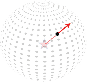
Figure 6.6
Sphere vertex normal vectors.
Some models define triangles using indices. Note in Figure 6.3 that each vertex appears in multiple triangles, which would lead to each vertex being specified multiple times. Rather than doing this, we instead store each vertex once, and then specify indices for each corner of a triangle, referencing the desired vertices. Since we will store a vertex’s location, texture coordinates, and normal vector, this can facilitate memory savings for large models.
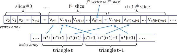
The vertices are stored in a one-dimensional array, starting with the vertices in the bottommost horizontal slice. When using indexing, the associated array of indices includes an entry for each triangle corner. The contents are integer references (specifically, subscripts) into the vertex array. Assuming that each slice contains n vertices, the vertex array would look as shown in Figure 6.7, along with an example portion of the corresponding index array.
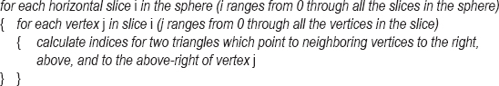
We can then traverse the vertices in a circular fashion around each horizontal slice, starting at the bottom of the sphere. As we visit each vertex, we build two triangles forming a square region above and to its right, as shown earlier in Figure 6.3. The processing is thus organized into nested loops, as follows:
Figure 6.7
Vertex array and corresponding index array.
For example, consider the “red” vertex from Figure 6.3 (repeated in Figure 6.8). The vertex in question is at the lower left of the yellow triangles shown in Figure 6.8, and given the loops just described, would be indexed by i*n+j, where i is the slice currently being processed (the outer loop), j is the vertex currently being processed within that slice (the inner loop), and n is the number of vertices per slice. Figure 6.8 shows this vertex (in red) along with its three relevant neighboring vertices, each with formulas showing how they would be indexed.
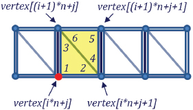
Figure 6.8
Indices generated for the jth vertex in the ith slice (n = number of vertices per slice).
These four vertices are then used to build the two triangles (shown in yellow) generated for this (red) vertex. The six entries in the index table for these two triangles are indicated in the figure in the order shown by the numbers 1 through 6. Note that entries 3 and 6 both refer to the same vertex, which is also the case for entries 2 and 4. The two triangles thus defined when we reach the vertex highlighted in red (i.e., vertex[i*n+j]) are built out of these six vertices—one with entries marked 1, 2, 3 referencing vertices vertex[i*n+j], vertex[i*n+j+1], and vertex[(i+1)*n+j], and one with entries marked 4, 5, 6 referencing the three vertices vertex[i*n+j+1], vertex[(i+1)*n+j+1], and vertex[(i+1)*n+j].
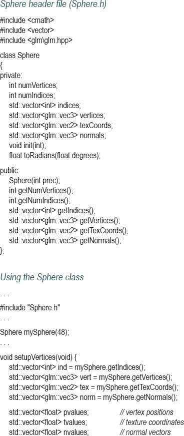
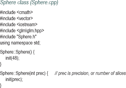
Program 6.1 shows the implementation of our sphere model as a class named Sphere. The center of the resulting sphere is at the origin. Code for using Sphere is also shown. Note that each vertex is stored in C++ vectors containing instances of the GLM classes vec2 and vec3 (this is different from previous examples, where vertices were stored in float arrays). vec2 and vec3 include methods for obtaining the desired x, y, and z components as float values, which are then put into float buffers as before. We store these values in variable-length C++ vectors because the size depends on the number of slices specified at runtime.
Note the calculation of triangle indices in the Sphere class, as described earlier in Figure 6.8. The variable “prec” refers to the “precision,” which in this case is used both for the number of sphere slices and the number of vertices per slice. Because the texture map wraps completely around the sphere, we will need an extra coincident vertex at each of the points where the left and right edges of the texture map meet. Thus, the total number of vertices is (prec+1)*(prec+1). Since six triangle indices are generated per vertex, the total number of indices is prec*prec*6.
Program 6.1 Procedurally Generated Sphere
When using the Sphere class, we will need three values for each vertex position and normal vector, but only two values for each texture coordinate. This is reflected in the declarations for the vectors (vertices, texCoords, and normals) shown in the Sphere.h header file, and from which the data is later loaded into the buffers.
It is important to note that although indexing is used in the process of building the sphere, the ultimate sphere vertex data stored in the VBOs doesn’t utilize indexing. Rather, as setupVertices() loops through the sphere indices, it generates separate (often redundant) vertex entries in the VBO for each of the index entries. OpenGL does have a mechanism for indexing vertex data; for simplicity we didn’t use it in this example, but we will use OpenGL’s indexing in the next example.
Figure 6.9 shows the output of Program 6.1, with a precision of 48. The texture from Figure 6.5 has been loaded as described in Chapter 5.

Figure 6.9
Textured sphere model.
Many other models can be created procedurally, from geometric shapes to real-world objects. One of the most well-known is the “Utah teapot” [CH16], which was developed in 1975 by Martin Newell, using a variety of Bézier curves and surfaces. The OpenGL Utility Toolkit (or “GLUT”) [GL16] even includes procedures for drawing teapots(!) (see Figure 6.10). We don’t cover GLUT in this book, but Bézier surfaces are covered in Chapter 11.

Figure 6.10
OpenGL GLUT teapot.
6.2OPENGL INDEXING – BUILDING A TORUS
6.2.1The Torus
Algorithms for producing a torus can be found on various websites. Paul Baker gives a step-by-step description for defining a circular slice, and then rotating the slice around a circle to form a donut [PP07]. Figure 6.11 shows two views, from the side and from above.
The way that the torus vertex positions are generated is rather different from what was done to build the sphere. For the torus, the algorithm positions a vertex to the right of the origin and then rotates that vertex in a circle on the XY plane using a rotation around the Z axis to form a “ring.” The ring is then moved outward by the “inner radius” distance. Texture coordinates and normal vectors are computed for each of these vertices as they are built. An additional vector tangent to the surface of the torus (called the tangent vector) is also generated for each vertex.
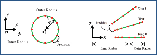
Figure 6.11
Building a torus.
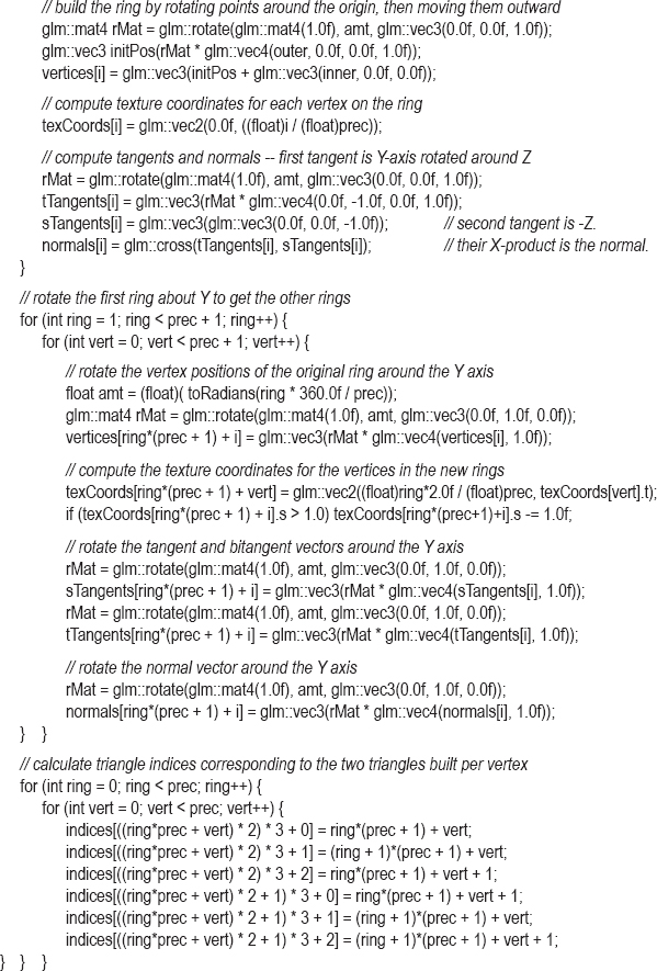
Vertices for additional torus rings are formed by rotating the original ring around the Y axis. Tangent and normal vectors for each resulting vertex are computed by also rotating the tangent and normal vectors of the original ring around the Y axis. After the vertices are created, they are traversed from ring to ring, and for each vertex two triangles are generated. The generation of six index table entries comprising the two triangles is done in a similar manner as we did for the sphere.
Our strategy for choosing texture coordinates for the remaining rings will be to arrange them so that the S axis of the texture image wraps halfway around the horizontal perimeter of the torus and then repeats for the other half. As we rotate around the Y axis generating the rings, we specify a variable ring that starts at 1 and increases up to the specified precision (again dubbed “prec”). We then set the S texture coordinate value to ring*2.0/prec, causing S to range between 0.0 and 2.0, then subtract 1.0 whenever the texture coordinate is greater than 1.0. The motivation for this approach is to avoid having the texture image appear overly “stretched” horizontally. If instead we did want the texture to stretch completely around the torus, we would simply remove the “*2.0” multiplier from the texture coordinate computation.
Building a torus class in C++/OpenGL could be done in a virtually identical manner as for the Sphere class. However, we have the opportunity to take advantage of the indices that we created while building the torus by using OpenGL’s support for vertex indexing (we could have also done this for the sphere, but we didn’t). For very large models with thousands of vertices, using OpenGL indexing can result in improved performance, and so we will describe how to do that next.
In both our sphere and torus models, we generate an array of integer indices referencing into the vertex array. In the case of the sphere, we use the list of indices to build a complete set of individual vertices and load them into a VBO just as we did for examples in earlier chapters. Instantiating the torus and loading its vertices, normals, and so on into buffers could be done in a similar manner as was done in Program 6.1, but instead we will use OpenGL’s indexing.
When using OpenGL indexing, we also load the indices themselves into a VBO. We generate one additional VBO for holding the indices. Since each index value is simply an integer reference, we first copy the index array into a C++ vector of integers, and then use glBufferData() to load the vector into the added VBO, specifying that the VBO is of type GL_ELEMENT_ARRAY_BUFFER (this tells OpenGL that the VBO contains indices). The code that does this can be added to setupVertices():
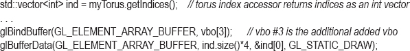
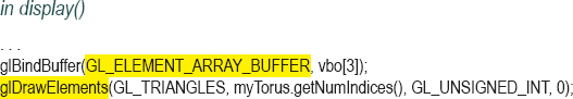
In the display() method, we replace the glDrawArrays() call with a call to glDrawElements(), which tells OpenGL to utilize the index VBO for looking up the vertices to be drawn. We also enable the VBO that contains the indices by using glBindBuffer(), specifying which VBO contains the indices and that it is a GL_ELEMENT_ARRAY_BUFFER. The code is as follows:
numTorusIndices = myTorus.getNumIndices();
glBindBuffer(GL_ELEMENT_ARRAY_BUFFER, vbo[3]);
glDrawElements(GL_TRIANGLES, numTorusIndices, GL_UNSIGNED_INT, 0);
Interestingly, the shaders used for drawing the sphere continue to work, unchanged, for the torus, even with the changes that we made in the C++/OpenGL application to implement indexing. OpenGL is able to recognize the presence of a GL_ELEMENT_ARRAY_BUFFER and utilize it to access the vertex attributes.
Program 6.2 shows a class named Torus based on Baker’s implementation. The “inner” and “outer” variables refer to the corresponding inner and outer radius in Figure 6.11. The prec (“precision”) variable has a similar role as in the sphere, with analogous computations for number of vertices and indices. By contrast, determining normal vectors is much more complex than it was for the sphere. We have used the strategy given in Baker’s description, wherein two tangent vectors are computed (dubbed sTangent and tTangent by Baker, although more commonly referred to as “tangent” and “bitangent”), and their cross-product forms the normal.
We will use this torus class (and the sphere class described earlier) in many examples throughout the remainder of the textbook.
Program 6.2 Procedurally Generated Torus
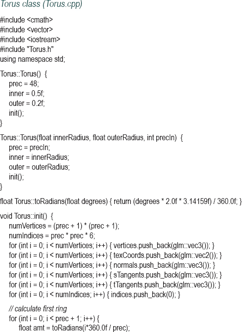
Note in the code that uses the Torus class that the loop in setupVertices() now stores the data associated with each vertex once, rather than once for each index entry (as was the case in the sphere example). This difference is also reflected in the declared array sizes for the data being entered into the VBOs. Also note that in the torus example, rather than using the index values when retrieving vertex data, they are simply loaded into VBO #3. Since that VBO is designated as a GL_ELEMENT_ARRAY_BUFFER, OpenGL knows that that VBO contains vertex indices.
Figure 6.12 shows the result of instantiating a torus and texturing it with the brick texture.
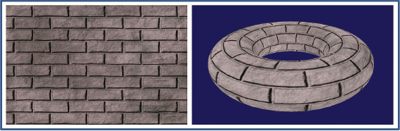
Figure 6.12
Procedurally generated torus.
6.3LOADING EXTERNALLY PRODUCED MODELS
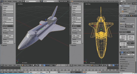
Complex 3D models, such as characters found in videogames or computer-generated movies, are typically produced using modeling tools. Such “DCC” (digital content creation) tools make it possible for people (such as artists) to build arbitrary shapes in 3D space and automatically produce the vertices, texture coordinates, vertex normals, and so on. There are too many such tools to list, but some examples are Maya, Blender, Lightwave, Cinema4D, and many others. Blender is free and open source. Figure 6.13 shows an example Blender screen during the editing of a 3D model.
Figure 6.13
Example Blender model creation [BL16].
In order for us to use a DCC-created model in our OpenGL scenes, that model needs to be saved (exported) in a format that we can read (import) into our program. There are several standard 3D model file formats; again, there are too many to list, but some examples are Wavefront (.obj), 3D Studio Max (.3ds), Stanford Scanning Repository (.ply), Ogre3D (.mesh), to name a few. Arguably the simplest is Wavefront (usually dubbed OBJ), so we will examine that one.
OBJ files are simple enough that we can develop a basic importer relatively easily. In an OBJ file, lines of text specify vertex geometric data, texture coordinates, normals, and other information. It has some limitations—for example, OBJ files have no way of specifying model animation.
Lines in an OBJ file start with a character tag indicating what kind of data is on that line. Some common tags include:
| • | v | – | geometric (vertex location) data |
| • | vt | – | texture coordinates |
| • | vn | – | vertex normal |
| • | f | – | face (typically vertices in a triangle) |
Other tags make it possible to store the object name, materials it uses, curves, shadows, and many other details. We will limit our discussion to the four tags listed above, which are sufficient for importing a wide variety of complex models.
Suppose we use Blender to build a simple pyramid such as the one we developed for Program 4.3. Figure 6.14 is a screenshot of a similar pyramid being created in Blender:
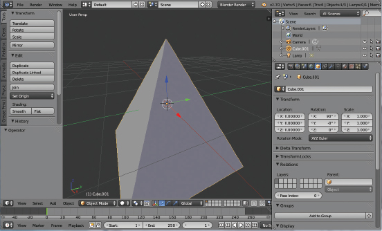
Figure 6.14
Pyramid built in Blender.
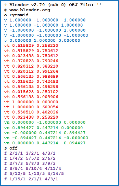
In Blender, if we now export our pyramid model, specify the .obj format, and also set Blender to output texture coordinates and vertex normals, an OBJ file is created that includes all of this information. The resulting OBJ file is shown in Figure 6.15. (The actual values of the texture coordinates can vary depending on how the model is built.)
We have color-coded the important sections of the OBJ file for reference. The lines at the top beginning with “#” are comments placed there by Blender, which our importer ignores. This is followed by a line beginning with “o” giving the name of the object. Our importer can ignore this line as well. Later, there is a line beginning with “s” that specifies that the faces shouldn’t be smoothed. Our code will also ignore lines starting with “s”.
The first substantive set of lines in the OBJ file are those starting with “v”, colored blue. They specify the X, Y, and Z local spatial coordinates of the five vertices of our pyramid model relative to the origin, which in this case is at the center of the pyramid.
Figure 6.15
Exported OBJ file for the pyramid.
The values colored red (starting with “vt”) are the various texture coordinates. The reason that the list of texture coordinates is longer than the list of vertices is that some of the vertices participate in more than one triangle, and in those cases different texture coordinates might be used.
The values colored green (starting with “vn”) are the various normal vectors. This list too is often longer than the list of vertices (although not in this example), again because some of the vertices participate in more than one triangle, and in those cases different normal vectors might be used.
The values colored purple (starting with “f”), near the bottom of the file, specify the triangles (i.e., “faces”). In this example, each face (triangle) has three elements, each with three values separated by “/” (OBJ allows other formats as well). The values for each element are indices into the lists of vertices, texture coordinates, and normal vectors respectively. For example, the third face is:
f 2 / 7 / 3 5 / 8 / 3 3 / 9 / 3
This indicates that the second, fifth, and third vertices from the list of vertices (in blue) comprise a triangle (note that OBJ indices start at 1). The corresponding texture coordinates are the seventh, eighth, and ninth from the list of texture coordinates in the section colored red. All three vertices have the same normal vector, the third in the list of normals in the section colored green.
Models in OBJ format are not required to have normal vectors, or even texture coordinates. If a model does not have texture coordinates or normals, the face values would specify only the vertex indices:
f 2 5 3
If a model has texture coordinates, but not normal vectors, the format would be as follows:
f 2 / 7 5 / 8 3 / 9
And, if the model has normals but not texture coordinates, the format would be:
f 2 / / 3 5 / / 3 3 / / 3
It is not unusual for a model to have tens of thousands of vertices. There are hundreds of such models available for download on the Internet for nearly every conceivable application, including models of animals, buildings, cars, planes, mythical creatures, people, and so on.
Programs of varying sophistication that can import an OBJ model are available on the Internet. Alternatively, it is relatively easy to write a very simple OBJ loader function that can handle the basic tags we have seen (v, vt, vn, and f). Program 6.3 shows one such loader, albeit a very limited one. It incorporates a class to hold an arbitrary imported model, which in turn calls the importer.
Before we describe the code in our simple OBJ importer, we must warn the reader of its limitations:
•It only supports models that include all three face attribute fields. That is, vertex positions, texture coordinates, and normals must all be present and in the form: f #/#/# #/#/# #/#/#.
•The material tag is ignored—texturing must be done using the methods described in Chapter 5.
•Only OBJ models composed of a single triangle mesh are supported (the OBJ format supports composite models, but our simple importer does not).
•It assumes that elements on each line are separated by exactly one space.
If you have an OBJ model that doesn’t satisfy all of the above criteria, and you wish to import it using the simple loader in Program 6.3, it may still be feasible to do so. It is often possible to load such a model into Blender, and then export it to another OBJ file that accommodates the loader’s limitations. For instance, if the model doesn’t include normal vectors, it is possible to have Blender produce normal vectors while it exports the revised OBJ file.
Another limitation of our OBJ loader has to do with indexing. Observe in the previous descriptions that the “face” tag allows for the possibility of mix-and-matching vertex positions, texture coordinates, and normal vectors. For example, two different “face” rows may include indices which point to the same v entry, but different vt entries. Unfortunately, OpenGL’s indexing mechanism does not support this level of flexibility—index entries in OpenGL can only point to a particular vertex along with its attributes. This complicates writing an OBJ model loader somewhat, as we cannot simply copy the references in the triangle face entries into an index array. Rather, using OpenGL indexing would require ensuring that entire combinations of v, vt, and vn values for a face entry each have their own references in the index array. A simpler, albeit less efficient, alternative is to create a new vertex for every triangle face entry. We opt for this simpler approach here in the interest of clarity, despite the space-saving advantage of using OpenGL indexing (especially when loading larger models).
The ModelImporter class includes a parseOBJ() function that reads in each line of an OBJ file one by one, handling separately the four cases v, vt, vn, and f. In each case, the subsequent numbers on the line are extracted, first by using erase() to skip the initial v, vt, vn, or f character(s), and then using the “>>” operator in the C++ stringstream class to extract each subsequent parameter value, and then storing them in a C++ float vector. As the face (f) entries are processed, the vertices are built with corresponding entries in C++ float vectors for vertex positions, texture coordinates, and normal vectors.
The ModelImporter class is included in the file containing the ImportedModel class, which simplifies loading and accessing the vertices of an OBJ file by putting the imported vertices into vectors of vec2 and vec3 objects. Recall these are GLM classes; we use them here to store vertex positions, texture coordinates, and normal vectors. The accessors in the ImportedModel class then make them available to the C++/OpenGL application in much the same manner as was done in the Sphere and Torus classes.
Following the ModelImporter and ImportedModel classes is an example sequence of calls for loading an OBJ file and then transferring the vertex information into a set of VBOs for subsequent rendering.
Figure 6.16 shows a rendered model of the space shuttle downloaded as an OBJ file from the NASA website [NA16], imported using the code from Program 6.3, and textured using the code from Program 5.1 with the associated NASA texture image file with anisotropic filtering. This texture image is an example of the use of UV-mapping, where texture coordinates in the model are carefully mapped to particular regions of the texture image. (As mentioned in Chapter 5, the details of UV-mapping are outside the scope of this book.)
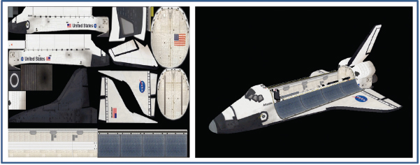
Figure 6.16
NASA space shuttle model with texture.
Program 6.3 Simple (Limited) OBJ Loader

SUPPLEMENTAL NOTES
Although we discussed the use of DCC tools for creating 3D models, we didn’t discuss how to use such tools. While such instruction is outside the scope of this text, there is a wealth of tutorial video material documentation for all of the popular tools such as Blender and Maya.
The topic of 3D modeling is itself a rich field of study. Our coverage in this chapter has been just a rudimentary introduction, with emphasis on its relationship to OpenGL. Many universities offer entire courses in 3D modeling, and readers interested in learning more are encouraged to consult some of the popular resources that offer greater detail (e.g., [BL16], [CH11], [VA12]).
We reiterate that the OBJ importer we presented in this chapter is limited, and can only handle a subset of the features supported by the OBJ format. Although sufficient for our needs, it will fail on some OBJ files. In those cases it would be necessary to first load the model into Blender (or Maya, etc.) and re-export it as an OBJ file that complies with the importer’s limitations as described earlier in this chapter.
Exercises
6.1Modify Program 4.4 so that the “sun,” “planet,” and “moon” are textured spheres, such as the ones shown in Figure 4.11.
6.2(PROJECT) Modify your program from Exercise 6.1 so that the imported NASA shuttle object from Figure 6.16 also orbits the “sun.” You’ll want to experiment with the scale and rotation applied to the shuttle to make it look realistic.
6.3(RESEARCH & PROJECT) Learn the basics of how to use Blender to create a 3D object of your own. To make full use of Blender with your OpenGL applications, you’ll want to learn how to use Blender’s UV-unwrapping tools to generate texture coordinates and an associated texture image. You can then export your object as an OBJ file and load it using the code from Program 6.3.
References
[BL16] |
Blender, The Blender Foundation, accessed October 2018, https://www.blender.org/ |
[CH11] |
A. Chopine, 3D Art Essentials: The Fundamentals of 3D Modeling, Texturing, and Animation (Focal Press, 2011). |
Computer History Museum, accessed October 2018, http://www.computerhistory.org/revolution/computer-graphics-music-and-art/15/206 | |
[GL16] |
GLUT and OpenGL Utility Libraries, accessed October 2018, https://www.opengl.org/resources/libraries/ |
[NA16] |
NASA 3D Resources, accessed October 2018, http://nasa3d.arc.nasa.gov/ |
[PP07] |
P. Baker, Paul’s Projects, 2007, accessed October 2018, www.paulsprojects.net |
[VA12] |
V. Vaughan, Digital Modeling (New Riders, 2012). |
[VE16] |
Visible Earth, NASA Goddard Space Flight Center Image, accessed October 2018, http://visibleearth.nasa.gov |