
MANAGING 3D GRAPHICS DATA
4.1Buffers and Vertex Attributes
4.3Interpolation of Vertex Attributes
4.4Model-View and Perspective Matrices
4.5Our First 3D Program – A 3D Cube
4.6Rendering Multiple Copies of an Object
4.7Rendering Multiple Different Models in a Scene
4.9Combating “Z-Fighting” Artifacts
4.10Other Options for Primitives

Using OpenGL to render 3D images generally involves sending several datasets through the OpenGL shader pipeline. For example, to draw a simple 3D object such as a cube, you will need to at least send the following items:
•the vertices for the cube model
•some transformation matrices to control the appearance of the cube’s orientation in 3D space
To complicate matters a bit, there are two ways of sending data through the OpenGL pipeline:
•through a buffer to a vertex attribute or
•directly to a uniform variable.
It is important to understand exactly how these two mechanisms work, so as to use the appropriate method for each item we are sending through.
Let’s start by rendering a simple cube.
4.1BUFFERS AND VERTEX ATTRIBUTES
For an object to be drawn, its vertices must be sent to the vertex shader. Vertices are usually sent by putting them in a buffer on the C++ side and associating that buffer with a vertex attribute declared in the shader. There are several steps to accomplish this, some of which only need to be done once, and some of which—if the scene is animated—must be done at every frame:
Done once—typically in init():
1.create a buffer
2.copy the vertices into the buffer
Done at each frame—typically in display():
1.enable the buffer containing the vertices
2.associate the buffer with a vertex attribute
3.enable the vertex attribute
4.use glDrawArrays(…) to draw the object
Buffers are typically created all at once at the start of the program, either in init() or in a function called by init(). In OpenGL, a buffer is contained in a Vertex Buffer Object, or VBO, which is declared and instantiated in the C++/OpenGL application. A scene may require many VBOs, so it is customary to generate and then fill several of them in init() so that they are available whenever your program needs to draw one or more of them.
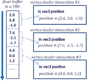
Figure 4.1
Data transmission between a VBO and a vertex attribute.
A buffer interacts with a vertex attribute in a specific way. When glDrawArrays() is executed, the data in the buffer starts flowing, sequentially from the beginning of the buffer, through the vertex shader. As described in Chapter 2, the vertex shader executes once per vertex. A vertex in 3D space requires three values, so an appropriate vertex attribute in the shader to receive these three values would be of type vec3. Then, for each three values in the buffer, the shader is invoked, as illustrated in Figure 4.1.
A related structure in OpenGL is called a Vertex Array Object, or VAO. VAOs were introduced in version 3.0 of OpenGL and are provided as a way of organizing buffers and making them easier to manipulate in complex scenes. OpenGL requires that at least one VAO be created, and for our purposes one will be sufficient.
For example, suppose that we wish to display two objects. On the C++ side, we could do this by declaring a single VAO and an associated set of two VBOs (one per object), as follows:
GLuint vao[1]; // OpenGL requires these values be specified in arrays
GLuint vbo[2];
…
glGenVertexArrays(1, vao);
glBindVertexArray(vao[0]);
glGenBuffers(2, vbo);
The two OpenGL commands glGenVertexArrays() and glGenBuffers() create VAOs and VBOs respectively, and return integer IDs for them. We store those IDs in the integer arrays vao and vbo. The two parameters on each of them refer to how many IDs are created, and an array to hold the returned IDs. The purpose of glBindVertexArrays() is to make the specified VAO “active” so that the generated buffers1 will be associated with that VAO.
A buffer needs to have a corresponding vertex attribute variable declared in the vertex shader. Vertex attributes are generally the first variables declared in a shader. In our cube example, a vertex attribute to receive the cube vertices could be declared in the vertex shader as follows:
layout (location = 0) in vec3 position;
The keyword in means “input” and indicates that this vertex attribute will be receiving values from a buffer (as we will see later, vertex attributes can also be used for “output”). As seen before, the “vec3” means that each invocation of the shader will grab three float values (presumably x, y, z, comprising a single vertex). The variable name is “position”. The “layout (location=0)” portion of the command is called a “layout qualifier” and is how we will associate the vertex attribute with a particular buffer. Thus this vertex attribute has an identifier 0 that we will use later for this purpose.
The manner in which we load the vertices of a model into a buffer (VBO) depends on where the model’s vertex values are stored. In Chapter 6 we will see how models are commonly built in a modeling tool (such as Blender [BL16] or Maya [MA16]), exported to a standard file format (such as .obj—also described in Chapter 6), and imported into the C++/OpenGL application. We will also see how a model’s vertices can be calculated on the fly or generated inside the pipeline using a tessellation shader.
For now, let’s say that we wish to draw a cube, and let’s presume that the vertices of our cube are hardcoded in an array in the C++/OpenGL application. In that case, we need to copy those values into one of our two buffers that we previously generated. To do that, we need to (a) make that buffer (say, the 0th buffer) “active” with the OpenGL glBindBuffer() command, and (b) use the glBufferData() command to copy the array containing the vertices into the active buffer (the 0th VBO in this case). Presuming that the vertices are stored in a float array named vPositions, the following C++ code2 would copy those values into the 0th VBO:
glBindBuffer(GL_ARRAY_BUFFER, vbo[0]);
glBufferData(GL_ARRAY_BUFFER, sizeof(vPositions), vPositions, GL_STATIC_DRAW);
Next, we add code to display() that will cause the values in the buffer to be sent to the vertex attribute in the shader. We do this with the following three steps: (a) make that buffer “active” with the glBindBuffer() command as we did above, (b) associate the active buffer with a vertex attribute in the shader, and (c) enable the vertex attribute. The following lines of code accomplish these steps:

Now when we execute glDrawArrays(), data in the 0th VBO will be transmitted to the vertex attribute that has a layout qualifier with location 0. This sends the cube vertices to the shader.
Rendering a scene so that it appears 3D requires building appropriate transformation matrices, such as those described in Chapter 3, and applying them to each of the models’ vertices. It is most efficient to apply the required matrix operations in the vertex shader, and it is customary to send these matrices from the C++/OpenGL application to the shader in a uniform variable.
Uniform variables are declared in a shader by using the “uniform” keyword. The following example, which declares variables to hold model-view and projection matrices, will be suitable for our cube program:
uniform mat4 mv_matrix;
uniform mat4 proj_matrix;
The keyword “mat4” indicates that these are 4x4 matrices. Here we have named the variable mv_matrix to hold the model-view matrix and the variable proj_matrix to hold the projection matrix. Since 3D transformations are 4x4, mat4 is a commonly used datatype in GLSL shader uniforms.
Sending data from a C++/OpenGL application to a uniform variable requires the following steps: (a) acquire a reference to the uniform variable and (b) associate a pointer to the desired values with the acquired uniform reference. Assuming that the linked rendering program is saved in a variable called “renderingProgram”, the following lines of code would specify that we will be sending model-view and projection matrices to the two uniforms mv_matrix and proj_matrix in our cube example:

The above example assumes that we have utilized the GLM utilities to build model-view and projection matrix transforms mvMat and pMat, as will be discussed in greater detail shortly. They are of type mat4 (a GLM class). The GLM function call value_ptr() returns a reference to the matrix data, which is needed by glUniformMatrix4fv() to transfer those matrix values to the uniform variable.
4.3INTERPOLATION OF VERTEX ATTRIBUTES
It is important to understand how vertex attributes are processed in the OpenGL pipeline, versus how uniform variables are processed. Recall that immediately before the fragment shader is rasterization, where primitives (e.g., triangles) defined by vertices are converted to fragments. Rasterization linearly interpolates vertex attribute values so that the displayed pixels seamlessly connect the modeled surfaces.
By contrast, uniform variables behave like initialized constants and remain unchanged across each vertex shader invocation (i.e., for each vertex sent from the buffer). A uniform variable is not interpolated; it always contains the same value regardless of the number of vertices.
The interpolation done on vertex attributes by the rasterizer is useful in many ways. Later, we will use rasterization to interpolate colors, texture coordinates, and surface normals. It is important to understand that all values sent through a buffer to a vertex attribute will be interpolated further down the pipeline.
We have seen vertex attributes in a vertex shader declared as “in” to indicate that they receive values from a buffer. Vertex attributes may instead be declared as “out”, meaning that they send their values forward toward the next stage in the pipeline. For example, the following declaration in a vertex shader specifies a vertex attribute named “color” that outputs a vec4:
out vec4 color;
It is not necessary to declare an “out” variable for the vertex positions, because OpenGL has a built-in out vec4 variable named gl_Position for that purpose. In the vertex shader, we apply the matrix transformations to the incoming vertex (declared earlier as position), assigning the result to gl_Position:
gl_Position = proj_matrix * mv_matrix * position;
The transformed vertices will then be automatically output to the rasterizer, with corresponding pixel locations ultimately sent to the fragment shader.
The rasterization process is illustrated in Figure 4.2. When specifying GL_TRIANGLES in the glDrawArrays() function, rasterization is done per triangle. Interpolation starts along the lines connecting the vertices, at a level of precision corresponding to the pixel display density. The pixels in the interior space of the triangle are then filled by interpolating along the horizontal lines connecting the edge pixels.
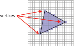
Figure 4.2
Rasterization of vertices.
4.4MODEL-VIEW AND PERSPECTIVE MATRICES
A fundamental step in rendering an object in 3D is to create appropriate transformation matrices and send them to uniform variables like we did in Section 4.2. We start by defining three matrices:
1.a Model matrix
2.a View matrix
3.a Perspective matrix
The Model matrix positions and orients the object in the world coordinate space. Each model has its own model matrix, and that matrix would need to be continuously rebuilt if the model moves.
The View matrix moves and rotates the models in the world to simulate the effect of a camera at a desired location. Recall from Chapter 2 that the OpenGL camera exists at location (0,0,0) and faces down the negative Z axis. To simulate the appearance of that camera being moved a certain way, we will need to move the objects themselves in the opposite direction. For example, moving a camera to the right would cause the objects in the scene to appear to move to the left; although the OpenGL camera is fixed, we can make it appear as though we have moved it to the right by moving the objects to the left.
The Perspective matrix is a transform that provides the 3D effect according to the desired frustum, as described earlier in Chapter 3.
It is also important to understand when to compute each type of matrix. Matrices that never change can be built in init(), but those that change would need to be built in display() so that they are rebuilt for each frame. Let’s assume that the models are animated and the camera is movable. Then:
•A model matrix needs to be created for each model and at each frame.
•The view matrix needs to be created once per frame (because the camera can be moved), but it is the same for all objects rendered during that frame.
•The perspective matrix is created once (in init()), using the screen window’s width and height (and desired frustum parameters), and it usually remains unchanged unless the window is resized.
Generating model and view transformation matrices then happens in the display() function, as follows:
1.Build the view matrix based on the desired camera location and orientation.
2.For each model, do the following:
i.Build a model matrix based on the model’s location and orientation.
ii.Concatenate the model and view matrices into a single “MV” matrix.
iii.Send the MV and projection matrices to the corresponding shader uniforms.
Technically, it isn’t necessary to combine the model and view matrices into a single matrix. That is, they could be sent to the vertex shader in individual, separate matrices. However, there are certain advantages to combining them, while keeping the perspective matrix separate. For example, in the vertex shader, each vertex in the model is multiplied by the matrices. Since complex models may have hundreds or even thousands of vertices, performance can be improved by pre-multiplying the model and view matrices once before sending them to the vertex shader. Later, we will see the need to keep the perspective matrix separate for lighting purposes.
4.5OUR FIRST 3D PROGRAM – A 3D CUBE
It’s time to put all the pieces together! In order to build a complete C++/OpenGL/GLSL system to render our cube in a 3D “world,” all of the mechanisms described so far will need to be put together and perfectly coordinated. We can reuse some of the code that we have seen previously in Chapter 2. Specifically, we won’t repeat the following functions for reading in files containing shader code, compiling and linking them, and detecting GLSL errors; in fact, recall that we have moved them to a “Utils.cpp” file:
•createShaderProgram()
•readShaderSource()
•checkOpenGLError()
•printProgramLog()
•printShaderLog()
We will also need a utility function that builds a perspective matrix, given a specified field-of-view angle for the Y axis, the screen aspect ratio, and the desired near and far clipping planes (selecting appropriate values for near and far clipping planes is discussed in Section 4.9). While we could easily write such a function ourselves, GLM already includes one:
glm::perspective(<field of view>, <aspect ratio>, <near plane>, <far plane>);
We now build the complete 3D cube program, shown as follows in Program 4.1:
Program 4.1 Plain Red Cube
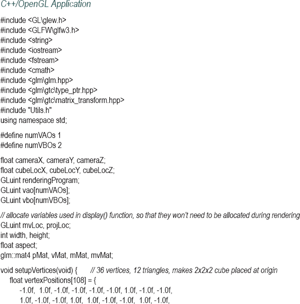
Let’s take a close look at the code in Program 4.1. It is important that we understand how all of the pieces work, and how they work together.

Figure 4.3
Output of Program 4.1. red cube positioned at (0,-2,0) viewed from (0,0,8).
Start by examining the function setupVertices(), called by init(). At the start of this function, an array is declared called vertexPositions that contains the 36 vertices comprising the cube. At first you might wonder why this cube has 36 vertices, when logically a cube should only require eight. The answer is that we need to build our cube out of triangles, and so each of the six cube faces needs to be built of two triangles, for a total of 6x2=12 triangles (see Figure 4.4). Since each triangle is specified by three vertices, this totals 36 vertices. Since each vertex has three values (x,y,z), there are a total of 36x3=108 values in the array. It is true that each vertex participates in multiple triangles, but we still specify each vertex separately because for now we are sending each triangle’s vertices down the pipeline separately.
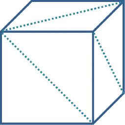
Figure 4.4
Cube made of triangles.
The cube is defined in its own coordinate system, with (0,0,0) at its center, and with its corners ranging from -1.0 to +1.0 along the x, y, and z axes. The rest of the " function sets up the VAO and two VBOs (although only one is used) and loads the cube vertices into the 0th VBO buffer.
Note that the init() function performs tasks that only need to be done once: reading in shader code and building the rendering program, and loading cube vertices into the VBO (by calling setupVertices()). Note that it also positions the cube and the camera in the world. Later we will animate the cube and also see how to move the camera around, at which point we may need to remove this hardcoded positioning.
Now let’s look at the display() function. Recall that display() may be called repeatedly and the rate at which it is called is referred to as the frame rate. That is, animation works by continually drawing and redrawing the scene, or frame, very quickly. It is usually necessary to clear the depth buffer before rendering a frame so that hidden surface removal occurs properly (not clearing the depth buffer can sometimes result in every surface being removed, resulting in a completely black screen). By default, depth values in OpenGL range from 0.0 to 1.0. Clearing the depth buffer is done by calling glClear(GL_DEPTH_BUFFER_BIT), which fills the depth buffer with the default value (usually 1.0).
Next, display() enables the shaders by calling glUseProgram(), installing the GLSL code on the GPU. Recall this doesn’t run the shader program, but it does enable subsequent OpenGL calls to determine the shader’s vertex attribute and uniform locations. The display() function next gets the uniform variable locations, builds the perspective, view, and model matrices3, concatenates the view and model matrices into a single MV matrix, and assigns the perspective and MV matrices to their corresponding uniforms. Here, it is worth noting also the form of the GLM call to the translate() function:
vMat = glm::translate(glm::mat4(1.0f), glm::vec3(-cameraX, -cameraY, -cameraZ));
The somewhat cryptic-looking call builds a translation matrix by (a) starting with an identity matrix (using the glm::mat4(1.0f) constructor) and (b) specifying translation values in the form of a vector (with the glm::vec3(x,y,z) constructor). Many of the GLM transform operations utilize this approach.
Next, display() enables the buffer containing the cube vertices and attaches it to 0th vertex attribute to prepare for sending the vertices to the shader.
The last thing display() does is draw the model by calling glDrawArrays(), specifying that the model is composed of triangles and has 36 total vertices. The call to glDrawArrays() is typically preceded by additional commands that adjust rendering settings for this model.4 In this example there are two such commands, both of which are related to depth testing. Recall from Chapter 2 that depth testing is used by OpenGL to perform hidden surface removal. Here, we enable depth testing and specify the particular depth test we wish OpenGL to use. The settings shown here correspond to the description in Chapter 2; later in the book we will see other uses for these commands.
Finally, consider the shaders. First, note that they both include the same block of uniform variable declarations. Although this is not always required, it is often a good practice to include the same block of uniform variable declarations in all of the shaders within a particular rendering program.
Note also in the vertex shader the presence of the layout qualifier on the incoming vertex attribute position. Since the location is specified as “0”, the display() function can reference this variable simply by using 0 in the first parameter of the glVertexAttribPointer() function call and in the glEnableVertexAttribArray() function call. Note also that the position vertex attribute is declared as a vec3, and so it needs to be converted to a vec4 in order to be compatible with the 4x4 matrices with which it will be multiplied. This conversion is done with vec4(position,1.0), which builds a vec4 out of the variable named “position”, putting a value of 1.0 in the newly added 4th spot.
The multiplication in the vertex shader applies the matrix transforms to the vertex, converting it to camera space (note the right-to-left concatenation order). Those values are put in the built-in OpenGL output variable gl_Position, and then proceed through the pipeline and are interpolated by the rasterizer.
The interpolated pixel locations (referred to as fragments) are then sent to the fragment shader. Recall that the primary purpose of the fragment shader is to set the color of an outputted pixel. In a manner similar to the vertex shader, the fragment shader processes the pixels one by one, with a separate invocation for each pixel. In this case, it outputs a hardcoded value corresponding to red. For reasons indicated earlier, the uniform variables have been included in the fragment shader even though they aren’t being used there in this example.
An overview of the flow of data starting with the C++/OpenGL application and passing through the pipeline is shown in Figure 4.5.
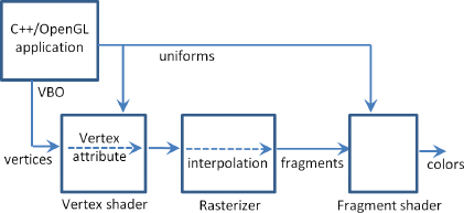
Figure 4.5
Data flow through Program 4.1.
Let’s make a slight modification to the shaders. In particular, we will assign a color to each vertex according to its location, and put that color in the outgoing vertex attribute varyingColor. The fragment shader is similarly revised to accept the incoming color (interpolated by the rasterizer) and use that to set the color of the output pixel. Note that the code also multiplies the location by 1/2 and then adds 1/2 to convert the range of values from [-1..+1] to [0..1]. Note also the use of the common convention of assigning variable names that include the word “varying” to programmer-defined interpolated vertex attributes. The changes in each shader are highlighted, and the resulting output is as follows.
Revised vertex shader:
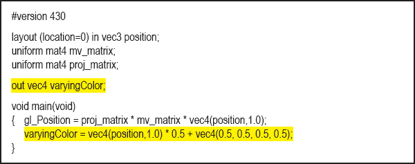
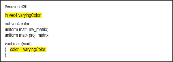

Figure 4.6
Cube with interpolated colors.
Note that because the colors are sent out from the vertex shader in a vertex attribute (varyingColor), they too are interpolated by the rasterizer! The effect of this can be seen in Figure 4.6, where the colors from corner to corner are clearly interpolated smoothly throughout the cube.
Note also that the “out” variable varyingColor in the vertex shader is also the “in” variable in the fragment shader. The two shaders know which variable from the vertex shader feeds which variable in the fragment shader because they have the same name “varyingColor” in both shaders.
Since our main() includes a render loop, we can animate our cube as we did in Program 2.6, by building the model matrix using a varying translation and rotation based on the time. For example, the code in the display() function in Program 4.1 could be modified as follows (changes are highlighted):
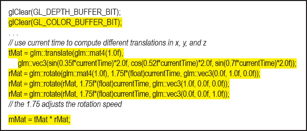
The use of current time (and a variety of trigonometric functions) in the model matrix causes the cube to appear to tumble around in space. Note that adding this animation illustrates the importance of clearing the depth buffer each time through display() to ensure correct hidden surface removal. It also necessitates clearing the color buffer as shown; otherwise, the cube will leave a trail as it moves.
The translate() and rotate() functions are part of the GLM library. Also, note the matrix multiplication in the last line—the order in which tMat and rMat are listed in the operation is significant. It computes a concatenation of the two transforms, with translation on the left and rotation on the right. When a vertex is subsequently multiplied by this matrix, the computation is right to left, meaning that the rotation is done first, followed by the translation. The order of application of transforms is significant, and changing the order would result in different behavior. Figure 4.7 shows some of the frames that are displayed after animating the cube.

Figure 4.7
Animated (“tumbling”) 3D cube.
4.6RENDERING MULTIPLE COPIES OF AN OBJECT
We now extend what we have learned to rendering multiple objects. Before we tackle the general case of rendering a variety of models in a single scene, let’s consider the simpler case of multiple occurrences of the same model. Suppose, for instance, that we wish to expand the previous example so that it renders a “swarm” of 24 tumbling cubes. We can do this by moving the portions of the code in display() that build the MV matrix and that draw the cube (shown as follows in blue) into a loop that executes 24 times. We incorporate the loop variable into the cube’s rotation and translation so that each time the cube is drawn, a different model matrix is built. (We also positioned the camera further down the positive Z axis so we can see all of the cubes.) A frame from the resulting animated scene is shown in Figure 4.8.
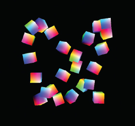
Figure 4.8
Multiple tumbling cubes.
4.6.1Instancing
Instancing provides a mechanism for telling the graphics card to render multiple copies of an object using only a single C++/OpenGL call. This can result in a significant performance benefit, particularly when there are thousands or millions of copies of the object being drawn—such as when rendering many flowers in a field, or many zombies in an army.
We start by changing the glDrawArrays() call in our C++/OpenGL application to glDrawArraysInstanced(). Now, we can ask OpenGL to draw as many copies as we want. We can specify drawing 24 cubes as follows:
glDrawArraysInstanced(GL_TRIANGLES, 0, 36, 24);
When using instancing, the vertex shader has access to a built-in variable gl_InstanceID, an integer that refers to which numeric instance of the object is currently being processed.
To replicate our previous tumbling cubes example using instancing, we will need to move the computations that build the different model matrices (previously inside a loop in display()) into the vertex shader. Since GLSL does not provide translate or rotate functions, and we cannot make calls to GLM from inside a shader, we will need to use the utility functions from Program 3.1. We will also need to pass the “time factor” from the C++/OpenGL application to the vertex shader in a uniform. We also need to pass the model and view matrices into separate uniforms because the rotation computations are applied to each cube’s model matrix. The revisions, including those in the C++/OpenGL application and those in the new vertex shader, are shown in Program 4.2.
Program 4.2 Instancing – Twenty-Four Animated Cubes
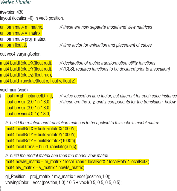
The resulting output of Program 4.2 is identical to that for the previous example, and can be seen in the previous Figure 4.8.
Instancing makes it possible to greatly expand the number of copies of an object; in this example animating 100,000 cubes is still feasible even for a modest GPU. The changes to the code—mainly just a few modified constants to spread the large number of cubes further apart—are as follows:
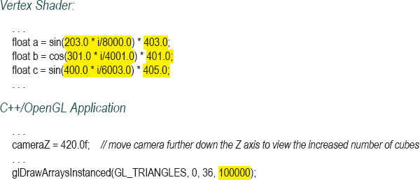
The resulting output is shown in Figure 4.9.
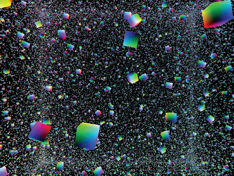
Figure 4.9
Instancing: 100,000 animated cubes.
4.7RENDERING MULTIPLE DIFFERENT MODELS IN A SCENE
To render more than one model in a single scene, a simple approach is to use a separate buffer for each model. Each model will need its own model matrix, and thus a new model-view matrix will be generated for each model that we render. There will also need to be separate calls to glDrawArrays() for each model. Thus there will need to be changes both in init() and in display().
Another consideration is whether or not we will need different shaders—or a different rendering program—for each of the objects we wish to draw. As it turns out, in many cases we can use the same shaders (and thus the same rendering program) for the various objects we are drawing. We usually only need to employ different rendering programs for the various objects if they are built of different primitives (such as lines instead of triangles), or if there are complex lighting or other effects involved. For now, that isn’t the case, so we can reuse the same vertex and fragment shaders, and just modify our C++/OpenGL application to send each model down the pipeline when display() is called.
Let’s proceed by adding a simple pyramid, so our scene includes both a single cube and a pyramid. The relevant modifications to the code are shown in Program 4.3. A few of the key details are highlighted, such as where we specify one or the other buffer, and where we specify the number of vertices contained in the model. Note that the pyramid is composed of six triangles—four on the sides and two on the bottom, totaling 6×3=18 vertices.
The resulting scene, containing both the cube and the pyramid, is then shown in Figure 4.10.
Program 4.3 Cube and Pyramid
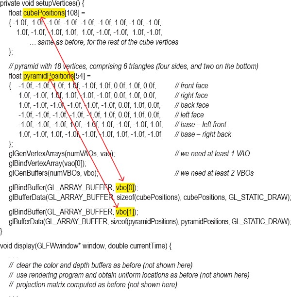
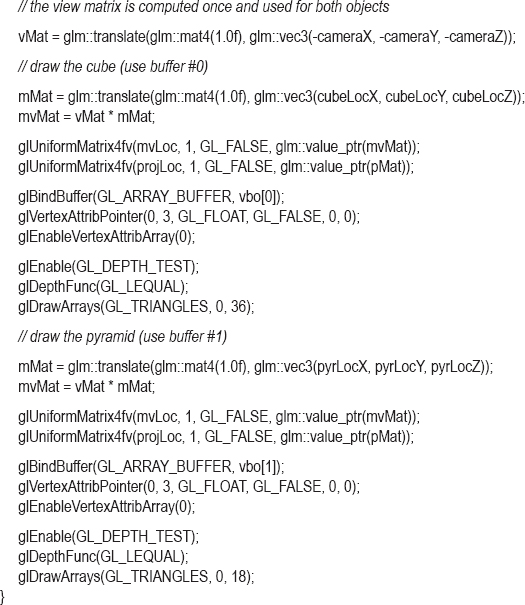
Figure 4.10
3D cube and pyramid.
A few other minor details to note regarding Program 4.3:
•The variables pyrLocX, pyrLocY, and pyrLocZ need to be declared and then initialized in init() to the desired pyramid location, as was done for the cube location.
•The view matrix vMat is built at the top of display() and then used in both the cube’s and the pyramid’s model-view matrices.
•The vertex and fragment shaders are not shown—they are unchanged from Section 4.5.
4.8MATRIX STACKS
So far, the models we have rendered have each been constructed of a single set of vertices. It is often desired, however, to build complex models by assembling smaller, simple models. For example, a model of a “robot” could be created by separately drawing the head, body, legs, and arms, where each of those is a separate model. An object built in this manner is often called a hierarchical model. The tricky part of building hierarchical models is keeping track of all the model-view matrices and making sure they stay perfectly coordinated—otherwise the robot might fly apart into pieces!
Hierarchical models are useful not only for building complex objects—they can also be used to generate complex scenes. For example, consider how our planet Earth revolves around the sun, and in turn how the moon revolves around the Earth. Such a scene is shown in Figure 4.11.5 Computing the moon’s actual path through space could be complex. However, if we can combine the transforms representing the two simple circular paths—the moon’s path around the Earth and the Earth’s path around the sun—we avoid having to explicitly compute the moon’s trajectory.
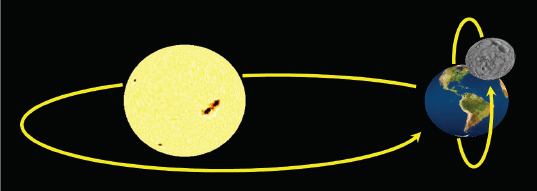
Figure 4.11
Animated planetary system (sun and earth textures from [HT16], moon texture from [NA16]).
It turns out that we can do this fairly easily with a matrix stack. A matrix stack is, as its name implies, a stack of transformation matrices. As we will see, matrix stacks make it easy to create and manage complex hierarchical objects and scenes, where transforms can be built upon (and removed from) other transforms.
OpenGL has a built-in matrix stack, but as part of the older fixed-function (non-programmable) pipeline it has long been deprecated [OL16]. However, the C++ Standard Template Library (STL) has a class called “stack” that is relatively straightforward to adapt as a matrix stack, by using it to build a stack of mat4s. As we will see, many of the model, view, and model-view matrices that would normally be needed in a complex scene can be replaced by a single instance of stack<glm::mat4>.
We will first examine the basic commands for instantiating and utilizing a C++ stack, then use one to build a complex animated scene. We will use the C++ stack class in the following ways:
•push() – makes available a new entry on the top of the stack. We will typically use this command by pushing a copy of the matrix that is currently at the top of the stack, with the intent of concatenating additional transforms onto the copy.
•pop() – removes (and returns) the top matrix.
•top() – returns a reference to the matrix at the top of the stack, without removing it.

As shown in the previous list, the “*=” operator is overloaded in mat4 so that it can be used to concatenate matrices. Therefore, we will typically use it in one of the forms shown to add translations, rotations, and so on to the matrix at the top of the matrix stack.
Now, rather than building transforms by creating instances of mat4, we instead use the push() command to create new matrices at the top of the stack. Desired transforms are then applied as needed to the newly created matrix on the top of the stack.
The first matrix pushed on the stack is frequently the VIEW matrix. The matrices above it are model-view matrices of increasing complexity; that is, they have an increasing number of model transforms applied to them. These transforms can either be applied directly or by first concatenating other matrices.
In our planetary system example, the matrix positioned immediately above the VIEW matrix would be the sun’s MV matrix. The matrix on top of that matrix would be the earth’s MV matrix, which consists of a copy of the sun’s MV matrix with the Earth’s model matrix transforms applied to it. That is, the Earth’s MV matrix is built by incorporating the planet’s transforms into the sun’s transforms. Similarly, the moon’s MV matrix sits on top of the planet’s MV matrix and is constructed by applying the moon’s model matrix transforms to the planet’s MV matrix immediately below it.
After rendering the moon, a second “moon” could be rendered by “popping” the first moon’s matrix off of the stack (restoring the top of the stack to the planet’s model-view matrix) and then repeating the process for the second moon.
The basic approach is as follows:
1.We declare our stack, giving it the name “mvStack”.
2.When a new object is created relative to a parent object, call “mvStack.push(mvStack.top())”.
3.Apply the new object’s desired transforms; i.e., multiply a desired transform onto it.
4.When an object or sub-object has finished being drawn, call “mvStack.pop()” to remove its model-view matrix from atop the matrix stack.
In later chapters we will learn how to create spheres and make them look like planets and moons. For now, to keep things simple, we will build a “planetary system” using our pyramid and a couple of cubes.
Here is an overview of how a display() function using a matrix stack is typically organized:
Note that the pyramid (“sun”) rotation on its axis is in its own local coordinate space, and should not be allowed to affect the “children” (the planet and moon, in this case). Therefore, the sun’s rotation (shown in the image below) is pushed onto the stack, but then after drawing the sun, it must be removed (popped) from the stack.
The big cube’s (planet) revolution around the sun (left image, below) will affect the moon’s movement, and so it is pushed on the stack and remains there when drawing the moon as well. By contrast, the planet’s rotation on its axis (right image, below) is local and does not affect the moon, so it is popped off the stack before drawing the moon.
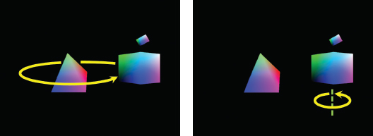
Similarly, we would push transforms onto the stack for the moon’s rotations (around the planet, and on its axis), indicated in the following images.

Here is the sequence of steps for the “planet”:
•push() This will be the portion of the planet’s MV matrix that will also affect children.
•translate(…) To incorporate the planet movement around the sun into the planet’s MV matrix. In this example we use trigonometry to calculate the planet movement as a translation.
•push() This will be the planet’s complete MV matrix, also including its axis rotation.
•rotate(…) To incorporate the planet’s axis rotation (this will later be popped and not affect children).
•glm::value_ptr(mvStack.top()) To obtain the MV matrix and then send it to the MV uniform.
•Draw the planet.
•pop()This removes the planet MV matrix off the stack, exposing underneath it an earlier copy of the planet MV matrix that doesn’t include the planet’s axis rotation (so that only the planet’s translation will affect the moon).
We now can write the complete display() routine, shown in Program 4.4.
Program 4.4 Simple Solar System Using Matrix Stack
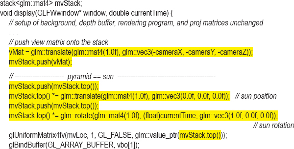
The matrix stack operations have been highlighted. There are several details worth noting:
•We have introduced a scale operation in a model matrix. We want the moon to be a smaller cube than the planet, so we use a call to scale() when building the MV matrix for the moon.
•In this example, we are using the trigonometric operations sin() and cos() to compute the revolution of the planet around the sun (as a translation), and also for the moon around the planet.
•The two buffers #0 and #1 contain cube and pyramid vertices respectively.
•Note the use of the glm::value_ptr(mvMatrix.top()) function call within the glUniformMatrix() command. This call retrieves the values in the matrix on top of the stack, and those values are then sent to the uniform variable (in this case, the sun, the planet, and then the moon’s MV matrices).
The vertex and fragment shaders are not shown—they are unchanged from the previous example. We also moved the initial position of the pyramid (sun) and the camera to center the scene on the screen.
4.9COMBATING “Z-FIGHTING” ARTIFACTS
Recall that when rendering multiple objects, OpenGL uses the Z-buffer algorithm (shown earlier in Figure 2.14) for performing hidden surface removal. Ordinarily, this resolves which object surfaces are visible and rendered to the screen, versus which surfaces lie behind other objects and thus should not be rendered, by choosing a pixel’s color to be that of the corresponding fragment closest to the camera.
However, there can be occasions when two object surfaces in a scene overlap and lie in coincident planes, making it problematic for the Z-buffer algorithm to determine which of the two surfaces should be rendered (since neither is “closest” to the camera). When this happens, floating point rounding errors can lead to some portions of the rendered surface using the color of one of the objects, and other portions using the color of the other object. This artifact is known as Z-fighting or depth-fighting, because the effect is the result of rendered fragments “fighting” over mutually corresponding pixel entries in the Z-buffer. Figure 4.12 shows an example of Z-fighting between two boxes with overlapping coincident (top) faces.
Figure 4.12
Z-fighting example.
Situations like this often occur when creating terrain or shadows. It is sometimes possible to predict Z-fighting in such instances, and a common way of correcting it in these cases is to move one object slightly, so that the surfaces are no longer coplanar. We will see an example of this in Chapter 8.
Z-fighting can also occur due to limited precision of the values in the depth buffer. For each pixel processed by the Z-buffer algorithm, the accuracy of its depth information is limited by the number of bits available for storing it in the depth buffer. The greater the range between near and far clipping planes used to build the perspective matrix, the more likely two objects’ points with similar (but not equal) actual depths will be represented by the same numeric value in the depth buffer. Therefore, it is up to the programmer to select near and far clipping plane values to minimize the distance between the two planes, while still ensuring that all objects essential to the scene lie within the viewing frustum.
It is also important to understand that, due to the effect of the perspective transform, changing the near clipping plane value can have a greater impact on the likelihood of Z-fighting artifacts than making an equivalent change in the far clipping plane. Therefore, it is advisable to avoid selecting a near clipping plane that is too close to the eye.
Previous examples in this book have simply used values of 0.1 and 1000 (in our calls to perspective()) for the near and far clipping planes. These may need to be adjusted for your scene.
4.10OTHER OPTIONS FOR PRIMITIVES
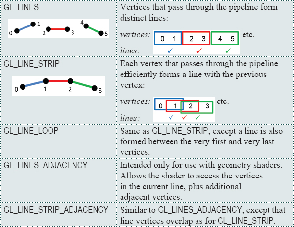
OpenGL supports a number of primitive types—so far we have seen two: GL_TRIANGLES and GL_POINTS. In fact, there are several others. All of the available primitive types supported in OpenGL fall into the categories of triangles, lines, points, and patches. Here is a complete list:
Line primitives:
Patch primitives:
GL_PATCH |
Intended only for use with tessellation shaders. Indicates that a set of vertices passes from the vertex shader to the tessellation control shader, where they are typically used to shape a tessellated grid into a curved surface. |
4.11CODING FOR PERFORMANCE
As the complexity of our 3D scenes grows, we will become increasingly concerned with performance. We have already seen a few instances where coding decisions were made in the interest of speed, such as when we used instancing, and when we moved expensive computations into the shaders.
Actually, the code we have presented has already also included some additional optimizations that we haven’t yet discussed. We now explore these and other important techniques.
4.11.1Minimizing Dynamic Memory Allocation
The critical section of our C++ code, with respect to performance, is clearly the display() function. This is the function that is called repeatedly during any animation or real-time rendering, and it is thus in this function (or in any function that it calls) where we must strive for maximum efficiency.
One important way of keeping overhead in the display() function to a minimum is by avoiding any steps that require memory allocation. Obvious examples of things to avoid thus would include:
•instantiating objects
•declaring variables
The reader is encouraged to review the programs that we have developed so far, and observe that virtually every variable used in the display() function was declared, and its space allocated, before the display() function was ever actually called. Declarations or instantiations almost never appear in display(). For example, Program 4.1 included the following block of code early in its listing:
// allocate variables used in display() function, so that they won’t need to be allocated during rendering
GLuint mvLoc, projLoc;
int width, height;
float aspect;
glm::mat4 pMat, vMat, mMat, mvMat;
Note that we purposely placed a comment at the top of the block indicating that these variables are pre-allocated for later use in the display() function (although we are only explicitly pointing that out now).
One case of a variable that wasnʼt pre-allocated occurred in our matrix stack example. By using the C++ stack class, each “push” operation results in a dynamic memory allocation. Interestingly in Java, the JOML library provides a MatrixStack class intended for use with OpenGL that allows one to pre-allocate space for a matrix stack! We utilize it in our Java-based “sister” book Computer Graphics Programming in OpenGL with Java, Second Edition.
There are other, more subtle examples. For example, function calls that convert data from one type to another may in some cases instantiate and return the newly converted data. It is thus important to understand the behaviors of any library functions called from display(). The math library, GLM, was not specifically designed with speed in mind. As a result, some of the operations can lead to dynamic allocation. We have tried to use GLM functions that operate directly onto (or into) variables whose space has already been allocated, when possible. The reader is encouraged to explore alternative methods when performance is critical.
4.11.2Pre-Computing the Perspective Matrix
Another optimization that can be done to reduce overhead in the display() function is to move the computation of the perspective matrix into the init() function. We mentioned this possibility earlier in Section 4.5 (well, in a footnote). While this is certainly easy to do, there is one slight complication. Although it is not normally necessary to recompute the perspective matrix, it would be necessary if the user running the application resizes the window (such as by dragging the window corner resize handle).
Fortunately, GLFW can be configured to automatically make a callback to a specified function whenever the window is resized. We add the following to the main(), just before the call to init():
glfwSetWindowSizeCallback(window, window_reshape_callback);
The first parameter is the GLFW window, and the second is the name of a function that GLFW calls whenever the window is resized. We then move the code that computes the perspective matrix into init(), and also copy it into a new function called window_reshape_callback().
Consider for example Program 4.1. If we reorganize the code so as to remove the computation of the perspective matrix from display(), then the revised versions of the main(), init(), display(), and the new function window_reshape_callback() would be as follows:
The implementations of the programs found on this book’s accompanying disk are all organized in this manner with respect to perspective matrix computation, starting with the interpolated colors version of Program 4.1.
4.11.3Back-Face Culling
Another way of improving rendering efficiency is to take advantage of OpenGL’s ability to do back-face culling. When a 3D model is entirely “closed,” meaning the interior is never visible (such as for the cube and for the pyramid), then it turns out that those portions of the outer surface that are angled away from the viewer will always be obscured by some other portion of the same model. That is, those triangles that face away from the viewer cannot possibly be seen (they would be overwritten by hidden surface removal anyway), and thus there is no reason to rasterize or render them.
We can ask OpenGL to identify and “cull” (not render) back-facing triangles with the command glEnable(GL_CULL_FACE). We can also disable face culling with glDisable(GL_CULL_FACE). By default, face culling is disabled, so if you want OpenGL to cull back-facing triangles, you must enable it.
When face culling is enabled, by default triangles are rendered only if they are front-facing. Also by default a triangle is considered front-facing if its three vertices progress in a counter-clockwise direction (based on the order that they were defined in the buffer) as viewed from the OpenGL camera. Triangles whose vertices progress in a clockwise direction (as viewed from the OpenGL camera) are back-facing, and are not rendered. This counter-clockwise definition of “front-facing” is sometimes called the winding order, and can be set explicitly using the function call glFrontFace(GL_CCW) for counter-clockwise (the default) or glFrontFace(GL_CW) for clockwise. Similarly, whether it is the front-facing or the back-facing triangles that are rendered can also be set explicitly. Actually, for this purpose we specify which ones are not to be rendered—that is, which ones are “culled.” We can specify that the back-facing triangles be culled (although this would be unnecessary because it is the default) by calling glCullFace(GL_BACK). Alternatively, we can specify instead that the front-facing triangles be culled, or even that all of the triangles be culled, by replacing the parameter GL_BACK with either GL_FRONT or GL_FRONT_AND_BACK respectively.
As we will see in Chapter 6, 3D models are typically designed so that the outer surface is constructed of triangles with the same winding order—most commonly counter-clockwise—so that if culling is enabled, then by default the portion of the model’s outer surface that faces the camera is rendered. Since by default OpenGL assumes the winding order is counter-clockwise, if a model is designed to be displayed with a clockwise winding order, it is up to the programmer to call gl_FrontFace(GL_CW) to account for this if back-face culling is enabled.
Note that in the case of GL_TRIANGLE_STRIP, the winding order of each triangle alternates. OpenGL compensates for this by “flipping” the vertex sequence when building each successive triangle, as follows: 0-1-2, then 2-1-3, 2-3-4, 4-3-5, 4-5-6, and so on.
Back-face culling improves performance by ensuring that OpenGL doesn’t spend time rasterizing and rendering surfaces that are never intended to be seen. Most of the examples we have seen in this chapter are so small that there is little motivation to enable face culling (an exception is the example shown in Figure 4.9, with the 100,000 instanced animated cubes, which may pose a performance challenge on some systems). In practice, it is common for most 3D models to be “closed,” and so it is customary to routinely enable back-face culling. For example, we can add back-face culling to Program 4.3 by modifying the display() function as follows:
Properly setting the winding order is important when using back-face culling. An incorrect setting, such as GL_CW when it should be GL_CCW, can lead to the interior of an object being rendered rather than its exterior, which in turn can produce distortion similar to that of an incorrect perspective matrix.
Efficiency isn’t the only reason for doing face culling. In later chapters we will see other uses, such as for those circumstances when we want to see the inside of a 3D model, or when using transparency.
SUPPLEMENTAL NOTES
There is a myriad of other capabilities and structures available for managing and utilizing data in OpenGL/GLSL, and we have only scratched the surface in this chapter. We haven’t, for example, described a uniform block, which is a mechanism for organizing uniform variables similar to a struct in C. Uniform blocks can even be set up to receive data from buffers. Another powerful mechanism is a shader storage block, which is essentially a buffer into which a shader can write.
An excellent reference on the many options for managing data is the OpenGL SuperBible [SW15], particularly the chapter entitled “Data” (Chapter 5 in the 7th edition). It also describes many of the details and options for the various commands that we have covered. The first two example programs in this chapter, Program 4.1 and Program 4.2, were inspired by similar examples in the SuperBible.
There are other types of data that we will need to learn how to manage, and how to send down the OpenGL pipeline. One of these is a texture, which contains color image data (such as in a photograph) that can be used to “paint” the objects in our scene. We will study texture images in Chapter 5. Another important buffer that we will study further is the depth buffer (or Z-buffer). This will become important when we study shadows in Chapter 8. We still have much to learn about managing graphics data in OpenGL!
Exercises
4.1(PROJECT) Modify Program 4.1 to replace the cube with some other simple 3D shape of your own design. Be sure to properly specify the number of vertices in the glDrawArrays() command.
4.2(PROJECT) In Program 4.1, the “view” matrix is defined in the display() function simply as the negative of the camera location:
vMat = glm::translate(glm::mat4(1.0f), glm::vec3(-cameraX, -cameraY, -cameraZ));
Replace this code with an implementation of the computation shown in Figure 3.13. This will allow you to position the camera by specifying a camera position and three orientation axes. You will find it necessary to store the vectors U,V,N described in Section 3.7. Then, experiment with different camera viewpoints, and observe the resulting appearance of the rendered cube.
4.3(PROJECT) Modify Program 4.4 to include a second “planet,” which is your custom 3D shape from Exercise 4.1. Make sure that your new “planet” is in a different orbit than the existing planet so that they don’t collide.
4.4(PROJECT) Modify Program 4.4 so that the “view” matrix is constructed using the “look-at” function (as described in Section 3.9). Then experiment with setting the “look-at” parameters to various locations, such as looking at the sun (in which case the scene should appear normal), looking at the planet, or looking at the moon.
4.5(RESEARCH) Propose a practical use for glCullFace(GL_FRONT_AND_BACK).
References
[BL16] |
Blender, The Blender Foundation, accessed October 2018, https://www.blender.org/ |
[HT16] |
J. Hastings-Trew, JHT’s Planetary Pixel Emporium, accessed October 2018, http://planetpixelemporium.com/ |
Maya, AutoDesk, Inc., accessed October 2018, http://www.autodesk.com/products/maya/overview | |
[NA16] |
NASA 3D Resources, accessed October 2018, http://nasa3d.arc.nasa.gov/ |
[OL16] |
Legacy OpenGL, accessed July 2016, https://www.opengl.org/wiki/Legacy_OpenGL |
[SW15] |
G. Sellers, R. Wright Jr., and N. Haemel, OpenGL SuperBible: Comprehensive Tutorial and Reference, 7th ed. (Addison-Wesley, 2015). |
1Throughout this example, two buffers are declared, to emphasize that usually we will use several buffers. Later we will use the additional buffer(s) to store other information associated with the vertex, such as color. In the current case we are using only one of the declared buffers, so it would have been sufficient to declare just one VBO.
2Note that here, for the first time, we are refraining from describing every parameter in one or more OpenGL calls. As mentioned in Chapter 2, the reader is encouraged to utilize the OpenGL documentation for such details as needed.
3An astute reader may notice that it shouldn’t be necessary to build the perspective matrix every time display() is called, because its value doesn’t change. This is partially true—the perspective matrix would need to be recomputed if the user were to resize the window while the program was running. In Section 4.11 we will handle this situation more efficiently, and in the process we will move the computation of the perspective matrix out of display() and into the init() function.
4Often, these calls may be placed in init() rather than in display(). However, it is necessary to place one or more of them in display() when drawing multiple objects with different properties. For simplicity, we always place them in display().
5Yes, we know that the moon doesn’t revolve in this “vertical” trajectory around the earth, but rather in one that is more co-planar with the earth’s revolution around the sun. We chose this orbit to make our program’s execution clearer.