THE OPENGL GRAPHICS PIPELINE
2.2Detecting OpenGL and GLSL Errors
2.3Reading GLSL Source Code from Files
2.4Building Objects from Vertices
2.6Organizing the C++ Code Files
OpenGL (Open Graphics Library) is a multi-platform 2D and 3D graphics API that incorporates both hardware and software. Using OpenGL requires a graphics card (GPU) that supports a sufficiently up-to-date version of OpenGL (as described in Chapter 1).
On the hardware side, OpenGL provides a multi-stage graphics pipeline that is partially programmable using a language called GLSL (OpenGL Shading Language).
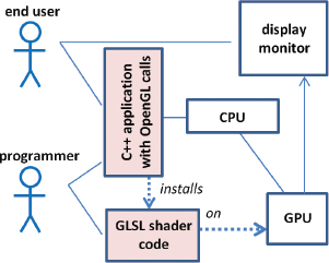
On the software side, OpenGL’s API is written in C, and thus the calls are directly compatible with C and C++. Stable language bindings (or “wrappers”) are available for more than a dozen other popular languages (Java, Perl, Python, Visual Basic, Delphi, Haskell, Lisp, Ruby, etc.) with virtually equivalent performance. This textbook uses C++, probably the most popular language choice. When using C++, the programmer writes code that runs on the CPU (compiled, of course) and includes OpenGL calls. We will refer to a C++ program that contains OpenGL calls as a C++/OpenGL application. One important task of a C++/OpenGL application is to install the programmer’s GLSL code onto the GPU.
An overview of a C++-based graphics application is shown in Figure 2.1, with the software components highlighted in pink.
Figure 2.1
Overview of a C++-based graphics application.
Some of the code we will write will be in C++, with OpenGL calls, and some will be written in GLSL. Our C++/OpenGL application will work together with our GLSL modules, and the hardware, to create our 3D graphics output. Once our application is complete, the end user will interact with the C++ application.
GLSL is an example of a shader language. Shader languages are intended to run on a GPU, in the context of a graphics pipeline. There are other shader languages, such as HLSL, which works with Microsoft’s 3D framework DirectX. GLSL is the specific shader language that is compatible with OpenGL, and thus we will write shader code in GLSL, in addition to our C++/OpenGL application code.
For the rest of this chapter, we will take a brief “tour” of the OpenGL pipeline. The reader is not expected to understand every detail thoroughly but should just get a feel for how the stages work together.
2.1THE OPENGL PIPELINE
Modern 3D graphics programming utilizes a pipeline, in which the process of converting a 3D scene to a 2D image is broken down into a series of steps. OpenGL and DirectX both utilize similar pipelines.
A simplified overview of the OpenGL graphics pipeline is shown in Figure 2.2 (not every stage is shown, just the major ones we will study). The C++/OpenGL application sends graphics data into the vertex shader—processing proceeds through the pipeline, and pixels emerge for display on the monitor.
The stages shaded in blue (vertex, tessellation, geometry, and fragment) are programmable in GLSL. It is one of the responsibilities of the C++/OpenGL application to load GLSL programs into these shader stages, as follows:
1.It uses C++ to obtain the GLSL shader code, either from text files or hardcoded as strings.
2.It then creates OpenGL shader objects and loads the GLSL shader code into them.
3.Finally, it uses OpenGL commands to compile and link objects and install them on the GPU.
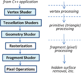
Figure 2.2
Overview of the OpenGL pipeline.
In practice, it is usually necessary to provide GLSL code for at least the vertex and fragment stages, whereas the tessellation and geometry stages are optional. Let’s walk through the entire process and see what takes place at each step.
2.1.1C++/OpenGL Application
The bulk of our graphics application is written in C++. Depending on the purpose of the program, it may interact with the end user using standard C++ libraries. For tasks related to 3D rendering, it uses OpenGL calls. As described in the previous chapter, we will be using several additional libraries: GLEW (OpenGL Extension Wrangler), GLM (OpenGL Mathematics), SOIL2 (Simple OpenGL Image Loader), and GLFW (Graphics Library Framework).
The GLFW library includes a class called GLFWwindow on which we can draw 3D scenes. As already mentioned, OpenGL also gives us commands for installing GLSL programs onto the programmable shader stages and compiling them. Finally, OpenGL uses buffers for sending 3D models and other related graphics data down the pipeline.
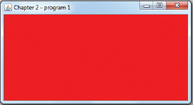
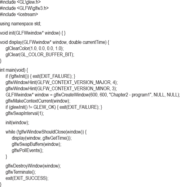
Before we try writing shaders, let’s write a simple C++/OpenGL application that instantiates a GLFWwindow and sets its background color. Doing that won’t require any shaders at all! The code is shown in Program 2.1. The main() function shown in Program 2.1 is the same one that we will use throughout this textbook. Among the significant operations in main() are: (a) initializes the GLFW library, (b) instantiates a GLFWwindow, (c) initializes the GLEW library, (d) calls the function “init()” once, and (e) calls the function “display()” repeatedly.
The “init()” function is where we will place application-specific initialization tasks. The display() method is where we place code that draws to the GLFWwindow. In this example, the glClearColor() command specifies the color value to be applied when clearing the background—in this case (1,0,0,1), corresponding to the RGB values of the color red (plus a “1” for the opacity component). We then use the OpenGL call glClear(GL_COLOR_BUFFER_BIT) to actually fill the color buffer with that color.
Program 2.1 First C++/OpenGL Application
The output of Program 2.1 is shown in Figure 2.3.
Figure 2.3
Output of Program 2.1.
The mechanism by which these functions are deployed is as follows: the GLFW and GLEW libraries are initialized using the commands glfwInit() and glewInit() respectively. The GLFW window and an associated OpenGL context1 are created with the glfwCreateWindow() command, with options set by any preceding window hints. Our window hints specify that the machine must be compatible with OpenGL version 4.3 (“major”=4. and “minor”=3). The parameters on the glfwCreateWindow() command specify the width and height of the window (in pixels) and the title placed at the top of the window. (The additional two parameters which are set to NULL, and which we aren’t using, allow for full screen mode and resource sharing.) Vertical synchronization (VSync) is enabled by using the glfwSwapInterval() and glfwSwapBuffers() commands—GLFW windows are by default double-buffered.2 Note that creating the GLFW window doesn’t automatically make the associated OpenGL context current—for that reason we also call glfwMakeContextCurrent().
Our main() includes a very simple rendering loop that calls our display() function repeatedly. It also calls glfwSwapBuffers(), which paints the screen, and glfwPollEvents(), which handles other window-related events (such as a key being pressed). The loop terminates when GLFW detects an event that should close the window (such as the user clicking the “X” in the upper right corner). Note that we have included a reference to the GLFW window object on the init() and display() calls; those functions may in certain circumstances need access to it. We have also included the current time on the call to display(), which will be useful for ensuring that our animations run at the same speed regardless of the computer being used. For this purpose, we use glfwGetTime(), which returns the elapsed time since GLFW was initialized.
Now is an appropriate time to take a closer look at the OpenGL calls in Program 2.1. Consider this one:
glClear(GL_COLOR_BUFFER_BIT);
In this case, the OpenGL function being called, as described in the OpenGL reference documentation (available on the web at https://www.opengl.org/sdk/docs), is:
void glClear(GLbitfield mask);
The parameter references a “GLbitfield” called “GL_COLOR_BUFFER_BIT”. OpenGL has many predefined constants (some of them are called enums); this one references the color buffer that contains the pixels as they are rendered. OpenGL has several color buffers, and this command clears all of them—that is, it fills them with a predefined color called the “clear color.” Note that “clear” in this context doesn’t mean “a color that is clear”; rather, it refers to the color that is applied when a color buffer is reset (cleared).
Immediately before the call to glClear() is a call to glClearColor(). This allows us to specify the value placed in the elements of a color buffer when it is cleared. Here we have specified (1,0,0,1), which corresponds to the RGBA color red.
Finally, our render loop exits when the user attempts to close the GLFW window. At that time, our main() asks GLFW to destroy the window and terminate, via calls to glfwDestroyWindow() and glfwTerminate() respectively.
2.1.2Vertex and Fragment Shaders
Our first OpenGL program didn’t actually draw anything—it simply filled the color buffer with a single color. To actually draw something, we need to include a vertex shader and a fragment shader.
You may be surprised to learn that OpenGL is capable of drawing only a few kinds of very simple things, such as points, lines, or triangles. These simple things are called primitives, and for this reason, most 3D models are made up of lots and lots of primitives, usually triangles.
Primitives are made up of vertices—for example, a triangle consists of three vertices. The vertices can come from a variety of sources—they can be read from files and then loaded into buffers by the C++/OpenGL application, or they can be hardcoded in the C++ code or even in the GLSL code.
Before any of this can happen, the C++/OpenGL application must compile and link appropriate GLSL vertex and fragment shader programs, and then load them into the pipeline. We will see the commands for doing this shortly.
The C++/OpenGL application also is responsible for telling OpenGL to construct triangles. We do this by using the following OpenGL function:
glDrawArrays(GLenum mode, Glint first, GLsizei count);
The mode is the type of primitive—for triangles we use GL_TRIANGLES. The parameter “first” indicates which vertex to start with (generally vertex number 0, the first one), and count specifies the total number of vertices to be drawn.
When glDrawArrays() is called, the GLSL code in the pipeline starts executing. Let’s now add some GLSL code to that pipeline.
Regardless of where they originate, all of the vertices pass through the vertex shader. They do so one by one; that is, the shader is executed once per vertex. For a large and complex model with a lot of vertices, the vertex shader may execute hundreds, thousands, or even millions of times, often in parallel.
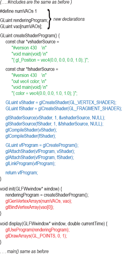
Let’s write a simple program with only one vertex, hardcoded in the vertex shader. That’s not enough to draw a triangle, but it is enough to draw a point. For it to display, we also need to provide a fragment shader. For simplicity we will declare the two shader programs as arrays of strings.
Program 2.2 Shaders, Drawing a POINT
The program appears to have output a blank window (see Figure 2.4). But close examination reveals a tiny blue dot in the center of the window (assuming that this printed page is of sufficient resolution). The default size of a point in OpenGL is one pixel.
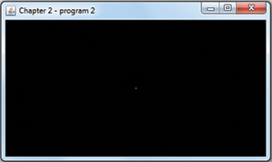
Figure 2.4
Output of Program 2.2.
There are many important details in Program 2.2 (color-coded in the program, for convenience) for us to discuss. First, note the frequent use of “GLuint”—this is a platform-independent shorthand for “unsigned int”, provided by OpenGL (many OpenGL constructs have integer references). Next, note that init() is no longer empty—it now calls another function named “createShaderProgram()” (that we wrote). This function starts by declaring two shaders as character strings called vshaderSource and fshaderSource. It then calls glCreateShader() twice, which generates the two shaders of types GL_VERTEX_SHADER and GL_FRAGMENT_SHADER. OpenGL creates each shader object (initially empty), and returns an integer ID for each that is an index for referencing it later—our code stores this ID in the variables vShader and fShader. It then calls glShaderSource(), which loads the GLSL code from the strings into the empty shader objects. The shaders are then each compiled using glCompileShader(). glShaderSource() has four parameters: (a) the shader object in which to store the shader, (b) the number of strings in the shader source code, (c) an array of pointers to strings containing the source code, and (d) an additional parameter we aren’t using (it will be explained later, in the supplementary chapter notes). Note that the two calls specify the number of lines of code in each shader as being “1”—this too is explained in the supplementary notes.
The application then creates a program object named vfProgram, and saves the integer ID that points to it. An OpenGL “program” object contains a series of compiled shaders, and here we see the following commands: glCreateProgram() to create the program object, glAttachShader() to attach each of the shaders to it, and then glLinkProgram() to request that the GLSL compiler ensure that they are compatible.
As we saw earlier, after init() finishes, display() is called. One of the first things display() does is call glUseProgram(), which loads the program containing the two compiled shaders into the OpenGL pipeline stages (onto the GPU!). Note that glUseProgram() doesn’t run the shaders, it just loads them onto the hardware.
As we will see later in Chapter 4, ordinarily at this point the C++/OpenGL program would prepare the vertices of the model being drawn for sending down the pipeline. But not in this case, because for our first shader program we simply hardcoded a single vertex in the vertex shader. Therefore in this example the display() function next proceeds to the glDrawArrays() call, which initiates pipeline processing. The primitive type is GL_POINTS, and there is just one point to display.
Now let’s look at the shaders themselves, shown in green earlier (and duplicated in the explanations that follow). As we saw, they have been declared in the C++/OpenGL program as arrays of strings. This is a clumsy way to code, but it is sufficient in this very simple case. The vertex shader is:
#version 430
void main(void)
{ gl_Position = vec4(0.0, 0.0, 0.0, 1.0); }
The first line indicates the OpenGL version, in this case 4.3. There follows a “main” function (as we will see, GLSL is somewhat C++-like in syntax). The primary purpose of any vertex shader is to send a vertex down the pipeline (which, as mentioned before, it does for every vertex). The built-in variable gl_Position is used to set a vertex’s coordinate position in 3D space, and is sent to the next stage in the pipeline. The GLSL datatype vec4 is used to hold a 4-tuple, suitable for such coordinates, with the associated four values representing X, Y, Z, and a fourth value set here to 1.0 (we will learn the purpose of this fourth value in Chapter 3). In this case, the vertex is hardcoded to the origin location (0,0,0).
The vertices move through the pipeline to the rasterizer, where they are transformed into pixel locations (or more accurately fragments—this is described later). Eventually, these pixels (fragments) reach the fragment shader:
#version 430
out vec4 color;
void main(void)
{ color = vec4(0.0, 0.0, 1.0, 1.0); }
The purpose of any fragment shader is to set the RGB color of a pixel to be displayed. In this case the specified output color (0, 0, 1) is blue (the fourth value 1.0 specifies the level of opacity). Note the “out” tag indicating that the variable color is an output. (It wasn’t necessary to specify an “out” tag for gl_Position in the vertex shader, because gl_Position is a predefined output variable.)
There is one detail in the code that we haven’t discussed, in the last two lines in the init() function (shown in red). They probably appear a bit cryptic. As we will see in Chapter 4, when sets of data are prepared for sending down the pipeline, they are organized into buffers. Those buffers are in turn organized into Vertex Array Objects (VAOs). In our example, we hardcoded a single point in the vertex shader, so we didn’t need any buffers. However, OpenGL still requires that at least one VAO be created whenever shaders are being used, even if the application isn’t using any buffers. So the two lines create the required VAO.
Finally, there is the issue of how the vertex that came out of the vertex shader became a pixel in the fragment shader. Recall from Figure 2.2 that between vertex processing and pixel processing is the rasterization stage. It is there that primitives (such as points or triangles) are converted into sets of pixels. The default size of an OpenGL “point” is one pixel, so that is why our single point was rendered as a single pixel.
Let’s add the following command in display(), right before the glDrawArrays() call:
glPointSize(30.0f);
Now, when the rasterizer receives the vertex from the vertex shader, it will set pixel color values that form a point having a size of 30 pixels. The resulting output is shown in Figure 2.5.
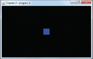
Figure 2.5
Changing glPointSize.
Let’s now continue examining the remainder of the OpenGL pipeline.
2.1.3Tessellation
We cover tessellation in Chapter 12. The programmable tessellation stage is one of the most recent additions to OpenGL (in version 4.0). It provides a tessellator that can generate a large number of triangles, typically as a grid, and also some tools to manipulate those triangles in a variety of ways. For example, the programmer might manipulate a tessellated grid of triangles as shown in Figure 2.6.
Tessellation is useful when a lot of vertices are needed on what is otherwise a simple shape, such as on a square area or curved surface. It is also very useful for generating complex terrain, as we will see later. In such instances, it is sometimes much more efficient to have the tessellator in the GPU generate the triangle mesh in hardware, rather than doing it in C++.
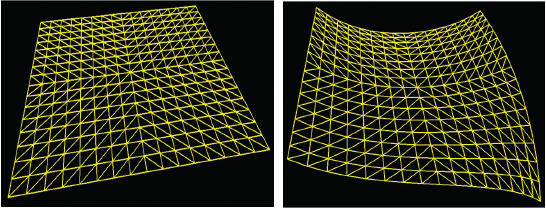
Figure 2.6
Grid produced by tessellator.
2.1.4Geometry Shader
We cover the geometry shader stage in Chapter 13. Whereas the vertex shader gives the programmer the ability to manipulate one vertex at a time (i.e., “per-vertex” processing), and the fragment shader (as we will see) allows manipulating one pixel at a time (“per-fragment” processing), the geometry shader provides the capability to manipulate one primitive at a time—“per-primitive” processing.
Recalling that the most common primitive is the triangle, by the time we have reached the geometry stage, the pipeline must have completed grouping the vertices into triangles (a process called primitive assembly). The geometry shader then makes all three vertices in each triangle accessible to the programmer simultaneously.
There are a number of uses for per-primitive processing. The primitives could be altered, such as by stretching or shrinking them. Some of the primitives could be deleted, thus putting “holes” in the object being rendered—this is one way of turning a simple model into a more complex one.
The geometry shader also provides a mechanism for generating additional primitives. Here too, this opens the door to many possibilities for turning simple models into more complex ones.
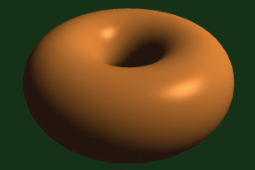
An interesting use for the geometry shader is for adding surface texture such as bumps or scales—even “hair” or “fur”—to an object. Consider for example the simple torus shown in Figure 2.7 (we will see how to generate this later in the book). The surface of this torus is built out of many hundreds of triangles. If at each triangle we use a geometry shader to add additional triangles that face outward, we get the result shown in Figure 2.8. This “scaly torus” would be computationally expensive to try and model from scratch in the C++/OpenGL application side.
It might seem redundant to provide a per-primitive shader stage when the tessellation stage(s) give the programmer access to all of the vertices in an entire model simultaneously. The difference is that tessellation only offers this capability in very limited circumstances—specifically when the model is a grid of triangles generated by the tessellator. It does not provide such simultaneous access to all the vertices of, say, an arbitrary model being sent in from C++ through a buffer.
Figure 2.7
Torus model.
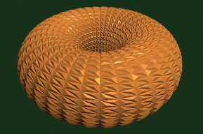
Figure 2.8
Torus modified in geometry shader.
2.1.5Rasterization
Ultimately, our 3D world of vertices, triangles, colors, and so on needs to be displayed on a 2D monitor. That 2D monitor screen is made up of a raster—a rectangular array of pixels.
When a 3D object is rasterized, OpenGL converts the primitives in the object (usually triangles) into fragments. A fragment holds the information associated with a pixel. Rasterization determines the locations of pixels that need to be drawn in order to produce the triangle specified by its three vertices.
Rasterization starts by interpolating, pairwise, between the three vertices of the triangle. There are some options for doing this interpolation; for now it is sufficient to consider simple linear interpolation as shown in Figure 2.9. The original three vertices are shown in red.
If rasterization were to stop here, the resulting image would appear as wireframe. This is an option in OpenGL, by adding the following command in the display() function, before the call to glDrawArrays():
glPolygonMode(GL_FRONT_AND_BACK, GL_LINE);
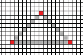
Figure 2.9
Rasterization (step 1).
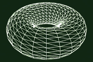
If the torus shown previously in Section 2.1.4 is rendered with the addition of this line of code, it appears as shown in Figure 2.10.
Figure 2.10
Torus with wireframe rendering.
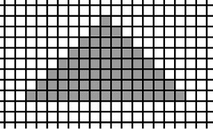
Figure 2.11
Fully rasterized triangle.
If we didn’t insert the preceding line of code (or if GL_FILL had been specified instead of GL_LINE), interpolation would continue along raster lines and fill the interior of the triangle, as shown in Figure 2.11. When applied to the torus, this results in the fully rasterized or “solid” torus shown in Figure 2.12 (on the left). Note that in this case the overall shape and curvature of the torus is not evident—that is because we haven’t included any texturing or lighting techniques, so it appears “flat.” At the right, the same “flat” torus is shown with the wireframe rendering superimposed. The torus shown earlier in Figure 2.7 included lighting effects, and thus revealed the shape of the torus much more clearly. We will study lighting in Chapter 7.
As we will see in later chapters, the rasterizer can interpolate more than just pixels. Any variable that is output by the vertex shader and input by the fragment shader will be interpolated based on the corresponding pixel position. We will use this capability to generate smooth color gradations, achieve realistic lighting, and many more effects.
2.1.6Fragment Shader
As mentioned earlier, the purpose of the fragment shader is to assign colors to the rasterized pixels. We have already seen an example of a fragment shader in Program 2.2. There, the fragment shader simply hardcoded its output to a specific value, so every generated pixel had the same color. However, GLSL affords us virtually limitless creativity to calculate colors in other ways.
One simple example would be to base the output color of a pixel on its location. Recall that in the vertex shader, the outgoing coordinates of a vertex are specified using the predefined variable gl_Position. In the fragment shader, there is a similar variable available to the programmer for accessing the coordinates of an incoming fragment, called gl_FragCoord. We can modify the fragment shader from Program 2.2 so that it uses gl_FragCoord (in this case referencing its x component using the GLSL field selector notation) to set each pixel’s color based on its location, as shown here:
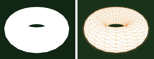
Figure 2.12
Torus with fully rasterized primitives (left), and with wireframe grid superimposed (right).
#version 430
out vec4 color;
void main(void)
{ if (gl_FragCoord.x < 200) color = vec4(1.0, 0.0, 0.0, 1.0); else color = vec4(0.0, 0.0, 1.0, 1.0);
}
Assuming that we increase the GL_PointSize as we did at the end of Section 2.1.2, the pixel colors will now vary across the rendered point—red where the x coordinates are less than 200, and blue otherwise, as seen in Figure 2.13.
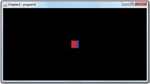
Figure 2.13
Fragment shader color variation.
2.1.7Pixel Operations
As objects in our scene are drawn in the display() function using the glDrawArrays() command, we usually expect objects in front to block our view of objects behind them. This also extends to the objects themselves, wherein we expect to see the front of an object, but generally not the back.
To achieve this, we need hidden surface removal, or HSR. OpenGL can perform a variety of HSR operations, depending on the effect we want in our scene. And even though this phase is not programmable, it is extremely important that we understand how it works. Not only will we need to configure it properly, we will later need to carefully manipulate it when we add shadows to our scene.
Hidden surface removal is accomplished by OpenGL through the cleverly coordinated use of two buffers: the color buffer (which we have discussed previously), and the depth buffer (sometimes called the Z-buffer). Both of these buffers are the same size as the raster—that is, there is an entry in each buffer for every pixel on the screen.
As various objects are drawn in a scene, pixel colors are generated by the fragment shader. The pixel colors are placed in the color buffer—it is the color buffer that is ultimately written to the screen. When multiple objects occupy some of the same pixels in the color buffer, a determination must be made as to which pixel color(s) are retained, based on which object is nearest the viewer.
Hidden surface removal is done as follows:
•Before a scene is rendered, the depth buffer is filled with values representing maximum depth.
•As a pixel color is output by the fragment shader, its distance from the viewer is calculated.
•If the computed distance is less than the distance stored in the depth buffer (for that pixel), then: (a) the pixel color replaces the color in the color buffer, and (b) the distance replaces the value in the depth buffer. Otherwise, the pixel is discarded.
This procedure is called the Z-buffer algorithm, as expressed in Figure 2.14.
2.2DETECTING OPENGL AND GLSL ERRORS
The workflow for compiling and running GLSL code differs from standard coding, in that GLSL compilation happens at C++ runtime. Another complication is that GLSL code doesn’t run on the CPU (it runs on the GPU), so the operating system cannot always catch OpenGL runtime errors. This makes debugging difficult, because it is often hard to detect if a shader failed, and why.

Figure 2.14
Z-buffer algorithm.
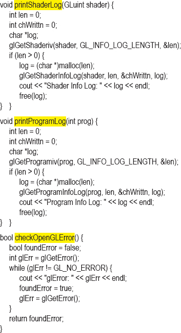
Program 2.3 (which follows) presents some modules for catching and displaying GLSL errors. They make use of the OpenGL functions glGetShaderiv() and glGetProgramiv(), which are used to provide information about compiled GLSL shaders and programs. Accompanying them is the createShaderProgram() function from the previous Program 2.2, but with the error-detecting calls added.
Program 2.3 contains the following three utilities:
•checkOpenGLError – checks the OpenGL error flag for the occurrence of an OpenGL error
•printShaderLog – displays the contents of OpenGL’s log when GLSL compilation failed
•printProgramLog – displays the contents of OpenGL’s log when GLSL linking failed
The first, checkOpenGLError(), is useful for detecting both GLSL compilation errors and OpenGL runtime errors, so it is highly recommended to use it throughout a C++/OpenGL application during development. For example, in the prior example (Program 2.2), the calls to glCompileShader() and glLinkProgram() could easily be augmented with the code shown in Program 2.3 to ensure that any typos or other compile errors would be caught and their cause reported. Calls to checkOpenGLError() could be added after runtime OpenGL calls, such as immediately after the call to glDrawArrays().
Another reason that it is important to use these tools is that a GLSL error does not cause the C++ program to stop. So unless the programmer takes steps to catch errors at the point that they happen, debugging will be very difficult.
Program 2.3 Modules to Catch GLSL Errors
Example of checking for OpenGL errors:

There are other tricks for deducing the causes of runtime errors in shader code. A common result of shader runtime errors is for the output screen to be completely blank, essentially with no output at all. This can happen even if the error is a very small typo in a shader, yet it can be difficult to tell at which stage of the pipeline the error occurred. With no output at all, it’s like looking for a needle in a haystack.
One useful trick in such cases is to temporarily replace the fragment shader with the one shown in Program 2.2. Recall that in that example, the fragment shader simply output a particular color—solid blue, for example. If the subsequent output is of the correct geometric form (but solid blue), the vertex shader is probably correct, and there is an error in the original fragment shader. If the output is still a blank screen, the error is more likely earlier in the pipeline, such as in the vertex shader.
In Appendix C we show how to use yet another useful debugging tool called Nsight, which is available for machines equipped with certain Nvidia graphics cards.
2.3READING GLSL SOURCE CODE FROM FILES
So far, our GLSL shader code has been stored inline in strings. As our programs grow in complexity, this will become impractical. We should instead store our shader code in files and read them in.
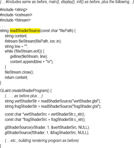
Reading text files is a basic C++ skill, and won’t be covered here. However, for practicality, code to read shaders is provided in readShaderSource(), shown in Program 2.4. It reads the shader text file and returns an array of strings, where each string is one line of text from the file. It then determines the size of that array based on how many lines were read in. Note that here, createShaderProgram() replaces the version from Program 2.2.
In this example, the vertex and fragment shader code is now placed in the text files “vertShader.glsl” and “fragShader.glsl” respectively.
Program 2.4 Reading GLSL Source from Files
2.4BUILDING OBJECTS FROM VERTICES
Ultimately we want to draw more than just a single point. We’d like to draw objects that are constructed of many vertices. Large sections of this book will be devoted to this topic. For now we just start with a simple example—we will define three vertices and use them to draw a triangle.
We can do this by making two small changes to Program 2.2 (actually, the version in Program 2.4 which reads the shaders from files): (a) modify the vertex shader so that three different vertices are output to the subsequent stages of the pipeline, and (b) modify the glDrawArrays() call to specify that we are using three vertices.
In the C++/OpenGL application (specifically in the glDrawArrays() call) we specify GL_TRIANGLES (rather than GL_POINTS), and also specify that there are three vertices sent through the pipeline. This causes the vertex shader to run three times, and at each iteration, the built-in variable gl_VertexID is automatically incremented (it is initially set to 0). By testing the value of gl_VertexID, the shader is designed to output a different point each of the three times it is executed. Recall that the three points then pass through the rasterization stage, producing a filled-in triangle. The modifications are shown in Program 2.5 (the remainder of the code is the same as previously shown in Program 2.4).
Program 2.5 Drawing a Triangle
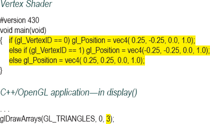

Figure 2.15
Drawing a simple triangle.
2.5ANIMATING A SCENE
Many of the techniques in this book can be animated. This is when things in the scene are moving or changing, and the scene is rendered repeatedly to reflect these changes in real time.
Recall from Section 2.1.1 that we have constructed our main() to make a single call to init(), and then to call display() repeatedly. Thus, while each of the preceding examples may have appeared to be a single fixed rendered scene, in actuality the loop in the main was causing it to be drawn over and over again.
For this reason, our main() is already structured to support animation. We simply design our display() function to alter what it draws over time. Each rendering of our scene is then called a frame, and the frequency of the calls to display() is the frame rate. Handling the rate of movement within the application logic can be controlled using the elapsed time since the previous frame (this is the reason for including “currentTime” as a parameter on the display() function).
An example is shown in Program 2.6. We have taken the triangle from Program 2.5 and animated it so that it moves to the right, then moves to the left, back and forth. In this example, we don’t consider the elapsed time, so the triangle may move more or less quickly depending on the speed of the computer. In future examples, we will use the elapsed time to ensure that our animations run at the same speed regardless of the computer on which they are run.
In Program 2.6, the application’s display() method maintains a variable “x” used to offset the triangle’s X coordinate position. Its value changes each time display() is called (and thus is different for each frame), and it reverses direction each time it reaches 1.0 or -1.0. The value in x is copied to a corresponding variable called “offset” in the vertex shader. The mechanism that performs this copy uses something called a uniform variable, which we will study later in Chapter 4. It isn’t necessary to understand the details of uniform variables yet. For now, just note that the C++/OpenGL application first calls glGetUniformLocation() to get a pointer to the “offset” variable, and then calls glProgramUniform1f() to copy the value of x into offset. The vertex shader then adds the offset to the X coordinate of the triangle being drawn. Note also that the background is cleared at each call to display(), to avoid the triangle leaving a trail as it moves. Figure 2.16 illustrates the display at three time instances (of course, the movement can’t be shown in a still figure).
Program 2.6 Simple Animation Example

Figure 2.16
An animated, moving triangle.
Note that in addition to adding code to animate the triangle, we have also added the following line at the beginning of the display() function:
glClear(GL_DEPTH_BUFFER_BIT);
While not strictly necessary in this particular example, we have added it here and it will continue to appear in most of our applications. Recall from the discussion in Section 2.1.7 that hidden surface removal requires both a color buffer and a depth buffer. As we proceed to drawing progressively more complex 3D scenes, it will be necessary to initialize (clear) the depth buffer each frame, especially for scenes that are animated, to ensure that depth comparisons aren’t affected by old depth data. It should be apparent from the previous example that the command for clearing the depth buffer is essentially the same as for clearing the color buffer.
2.6ORGANIZING THE C++ CODE FILES
So far, we have been placing all of the C++/OpenGL application code in a single file called “main.cpp”, and the GLSL shaders into files called “vertShader.glsl” and “fragShader.glsl”. While we admit that stuffing a lot of application code into main.cpp isn’t a best practice, we have adopted this convention in this book so that it is absolutely clear in every example which file contains the main block of C++/OpenGL code relevant to the example being discussed. Throughout this textbook, it will always be called “main.cpp”. In practice, applications should of course be modularized to appropriately reflect the tasks performed by the application.
However, as we proceed, there will be circumstances in which we create modules that will be useful in many different applications. Wherever appropriate, we will move those modules into separate files to facilitate reuse. For example, later we will define a Sphere class that will be useful in many different examples, and so it will be separated into its own files (Sphere.cpp and Sphere.h).
Similarly, as we encounter functions that we wish to reuse, we will place them in a file called “Utils.cpp” (and an associated “Utils.h”). We have already seen several functions that are appropriate to move into “Utils.cpp”: the error-detecting modules described in Section 2.2, and the functions for reading in GLSL shader programs described in Section 2.3. The latter is particularly well-suited to overloading, such that a “createShaderProgram()” function can be defined for each possible combination of pipeline shaders assembled in a given application:
•GLuint Utils::createShaderProgram(const char *vp, const char *fp)
•GLuint Utils::createShaderProgram(const char *vp, const char *gp, const char *fp)
•GLuint Utils::createShaderProgram(const char *vp, const char *tCS, const char* tES, const char *fp)
•GLuint Utils::createShaderProgram(const char *vp, const char *tCS, const char* tES, const char *gp, const char *fp)
The first case in the previous list supports shader programs which utilize only a vertex and fragment shader. The second supports those utilizing vertex, geometry, and fragment shaders. The third supports those using vertex, tessellation, and fragment shaders. And the fourth supports those using vertex, tessellation, geometry, and fragment shaders. The parameters accepted in each case are pathnames for the GLSL files containing the shader code. For example, the following call uses one of the overloaded functions to compile and link a shader pipeline program that includes a vertex and fragment shader. The completed program is placed in the variable “renderingProgram”:
renderingProgram = Utils::createShaderProgram("vertShader.glsl", "fragShader.glsl");

These createShaderProgram() implementations can all be found on the accompanying CD (in the “Utils.cpp” file), and all of them incorporate the error-detecting modules from Section 2.2 as well. There is nothing new about them; they are simply organized in this way for convenience. As we move forward in the book, other similar functions will be added to Utils.cpp as we go along. The reader is strongly encouraged to examine the Utils.cpp file on the accompanying CD, and even add to it as desired. The programs found there are built from the methods as we learn them in the book, and studying their organization should serve to strengthen one’s own understanding.
Regarding the functions in the “Utils.cpp” file, we have implemented them as static methods so that it isn’t necessary to instantiate the Utils class. Readers may prefer to implement them as instance methods rather than static methods, or even as freestanding functions, depending on the architecture of the particular system being developed.
All of our shaders will be named with a “.glsl” extension.
SUPPLEMENTAL NOTES
There are many details of the OpenGL pipeline that we have not discussed in this introductory chapter. We have skipped a number of internal stages and have completely omitted how textures are processed. Our goal was to map out, as simply as possible, the framework in which we will be writing our code. As we proceed we will continue to learn additional details.
We have also deferred presenting code examples for tessellation and geometry. In later chapters we will build complete systems that show how to write practical shaders for each of the stages.
There are more sophisticated ways to organize the code for animating a scene, especially with respect to managing threads. Some language bindings such as JOGL and LWJGL (for Java) offer classes to support animation. Readers interested in designing a render loop (or “game loop”) appropriate for a particular application are encouraged to consult some of the more specialized books on game engine design (e.g., [NY14]), and to peruse the related discussions on gamedev.net [GD17].
We glossed over one detail on the glShaderSource() command. The fourth parameter is used to specify a “lengths array” that contains the integer string lengths of each line of code in the given shader program. If this parameter is set to null, as we have done, OpenGL will build this array automatically if the strings are null-terminated. While we have been careful to ensure that our strings sent to glShaderSource() are null-terminated (by calling the c_str() function in createShaderProgram()), it is not uncommon to encounter applications that build these arrays manually rather than sending null.
Throughout this book, the reader may at times wish to know one or more of OpenGL’s upper limits. For example, the programmer might need to know the maximum number of outputs that can be produced by the geometry shader, or the maximum size that can be specified for rendering a point. Many such values are implementation-dependent, meaning that they can vary between different machines. OpenGL provides a mechanism for retrieving such limits using the glGet() command, which takes various forms depending on the type of the parameter being queried. For example, to find the maximum allowable point size, the following call will place the minimum and maximum values (for your machine’s OpenGL implementation) into the first two elements of the float array named “size”:
glGetFloatv(GL_POINT_SIZE_RANGE, size)
Many such queries are possible. Consult the OpenGL reference [OP16] documentation for examples.
In this chapter, we have tried to describe each parameter on each OpenGL call. However, as the book proceeds, this will become unwieldy and we will sometimes not bother describing a parameter when we believe that doing so would complicate matters unnecessarily. This is because many OpenGL functions have a large number of parameters that are irrelevant to our examples. The reader should get used to using the OpenGL documentation to fill in such details when necessary.
2.1Modify Program 2.2 to add animation that causes the drawn point to grow and shrink, in a cycle. Hint: use the glPointSize() function, with a variable as the parameter.
2.2Modify Program 2.5 so that it draws an isosceles triangle (rather than the right triangle shown in Figure 2.15).
2.3(PROJECT) Modify Program 2.5 to include the error-checking modules shown in Program 2.3. After you have that working, try inserting various errors into the shaders and observing both the resulting behavior and the error messages generated.
References
[GD17] |
Game Development Network, accessed October 2018, https://www.gamedev.net/ |
[NY14] |
R. Nystrom, “Game Loop,” in Game Programming Patterns (Genever Benning, 2014), and accessed October 2018, http://gameprogrammingpatterns.com/game-loop.html |
[OP16] |
OpenGL 4.5 Reference Pages, accessed July 2016, https://www.opengl.org/sdk/docs/man/ |
[SW15] |
G. Sellers, R. Wright Jr., and N. Haemel, OpenGL SuperBible: Comprehensive Tutorial and Reference, 7th ed. (Addison-Wesley, 2015). |
1The term “context” refers to an OpenGL instance and its state information, which includes items such as the color buffer.
2“Double buffering” means that there are two color buffers—one that is displayed, and one that is being rendered to. After an entire frame is rendered, the buffers are swapped. Double buffering is used to reduce undesirable visual artifacts.