
LIGHTING
7.6Combining Lighting and Textures

Light affects the appearance of our world in varied and sometimes dramatic ways. When a flashlight shines on an object, we expect it to appear brighter on the side facing the light. The earth on which we live is itself brightly lit where it faces the sun at noon, but as it turns, that daytime brightness gradually fades into evening, until becoming completely dark at midnight.
Objects also respond differently to light. Besides having different colors, objects can have different reflective characteristics. Consider two objects, both green, but where one is made of cloth versus another made of polished steel—the latter will appear more “shiny.”
7.1LIGHTING MODELS
Light is the product of photons being emitted by high energy sources and subsequently bouncing around until some of the photons reach our eyes. Unfortunately, it is computationally infeasible to emulate this natural process, as it would require simulating and then tracking the movement of a huge number of photons, adding many objects (and matrices) to our scene. What we need is a lighting model.
Lighting models are sometimes called shading models, although in the presence of shader programming, that can be a bit confusing. Sometimes the term reflection model is used, complicating the terminology further. We will try to stick to whichever terminology is simple and most practical.
The most common lighting models today are called “ADS” models, because they are based on three types of reflection labeled A, D, and S:
•Ambient reflection simulates a low-level illumination that equally affects everything in the scene.
•Diffuse reflection brightens objects to various degrees depending on the light’s angle of incidence.
•Specular reflection conveys the shininess of an object by strategically placing a highlight of appropriate size on the object’s surface where light is reflected most directly toward our eyes.
ADS models can be used to simulate different lighting effects and a variety of materials.
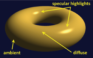
Figure 7.1
ADS Lighting contributions.
Figure 7.1 illustrates the ambient, diffuse, and specular contributions of a positional light on a shiny gold torus.
Recall that a scene is ultimately drawn by having the fragment shader output a color for each pixel on the screen. Using an ADS lighting model requires specifying contributions due to lighting on a pixel’s RGBA output value. Factors include:
•The type of light source and its ambient, diffuse, and specular characteristics
•The object’s material’s ambient, diffuse, and specular characteristics
•The object’s material’s specified “shininess”
•The angle at which the light hits the object
•The angle from which the scene is being viewed
There are many types of lights, each with different characteristics and requiring different steps to simulate their effects. Some types include:
•Global (usually called “global ambient” because it includes only an ambient component)
•Directional (or “distant”)
•Positional (or “point source”)
•Spotlight
Global ambient light is the simplest type of light to model. Global ambient light has no source position—the light is equal everywhere, at each pixel on every object in the scene, regardless of where the objects are. Global ambient lighting simulates the real-world phenomenon of light that has bounced around so many times that its source and direction are undeterminable. Global ambient light has only an ambient component, specified as an RGBA value; it has no diffuse or specular components. For example, global ambient light can be defined as follows:
float globalAmbient[4] = { 0.6f, 0.6f, 0.6f, 1.0f };
RGBA values range from 0 to 1, so global ambient light is usually modeled as dim white light, where each of the RGB values is set to the same fractional value between 0 and 1 and the alpha is set to 1.
Directional or distant light also doesn’t have a source location, but it does have a direction. It is useful for situations where the source of the light is so far away that the light rays are effectively parallel, such as light coming from the sun. In many such situations we may only be interested in modeling the light and not the object that produces the light. The effect of directional light on an object depends on the light’s angle of impact; objects are brighter on the side facing a directional light than on a tangential or opposite side. Modeling directional light requires specifying its direction (as a vector) and its ambient, diffuse, and specular characteristics (as RGBA values). A red directional light pointing down the negative Z axis might be specified as follows:
float dirLightAmbient[4] = { 0.1f, 0.0f, 0.0f, 1.0f };
float dirLightDiffuse[4] = { 1.0f, 0.0f, 0.0f, 1.0f };
float dirLightSpecular[4] = { 1.0f, 0.0f, 0.0f, 1.0f };
float dirLightDirection[4] = { 0.0f, 0.0f, -1.0f };
It might seem redundant to include an ambient contribution for a light when we already have global ambient light. The separation of the two, however, is intentional and noticeable when the light is “on” or “off.” When “on,” the total ambient contribution would be increased, as expected. In the above example, we have included only a small ambient contribution for the light. It is important to balance the two contributions depending on the needs of your scene.
A Positional light has a specific location in the 3D scene. Light sources that are near the scene, such as lamps, candles, and so forth, are examples. Like directional lights, the effect of a positional light depends on angle of impact; however, its direction is not specified, as it is different for each vertex in our scene. Positional lights may also incorporate attenuation factors in order to model how their intensity diminishes with distance. As with the other types of lights we have seen, positional lights have ambient, diffuse, and specular properties specified as RGBA values. A red positional light at location (5, 2, -3) could for example be specified as follows:
float posLightAmbient[4] = { 0.1f, 0.0f, 0.0f, 1.0f };
float posLightDiffuse[4] = { 1.0f, 0.0f, 0.0f, 1.0f };
float posLightSpecular[4] = { 1.0f,0.0f, 0.0f, 1.0f };
float posLightLocation[4] = { 5.0f, 2.0f, -3.0f };
Attenuation factors can be modeled in a variety of ways. One way is to include tunable non-negative parameters for constant, linear, and quadratic attenuation (kc, kl, and kq respectively). These parameters are then combined, taking into account the distance (d) from the light source:

Multiplying this factor by the light intensity causes the intensity to be decreased the greater the distance is to the light source. Note that kc should always be set greater than or equal to 1 so that the attenuation factor will always be in the range [0..1] and approach 0 as the distance d increases.
Spotlights have both a position and a direction. The effect of the spotlight’s “cone” can be simulated using a cutoff angle θ between 0° and 90° specifying the half-width of the light beam, and a falloff exponent to model the variation of intensity across the angle of the beam. As shown in Figure 7.2, we determine the angle ϕ between the spotlight’s direction and a vector from the spotlight to the pixel. We then compute an intensity factor by raising the cosine of ϕ to the falloff exponent when ϕ is less than θ (when ϕ is greater than θ, the intensity factor is set to 0). The result is an intensity factor that ranges from 0 to 1. The falloff exponent adjusts the rate at which the intensity factor tends to 0 as the angle ϕ increases. The intensity factor is then multiplied by the light’s intensity to simulate the cone effect.
A red spotlight at location (5,2,-3) pointing down the negative Z axis could be specified as:
float spotLightAmbient[4] = { 0.1f, 0.0f, 0.0f, 1.0f };
float spotLightDiffuse[4] = { 1.0f, 0.0f, 0.0f, 1.0f };
float spotLightSpecular[4] = { 1.0f,0.0f, 0.0f, 1.0f };
float spotLightLocation[3] = { 5.0f, 2.0f, -3.0f };
float spotLightDirection[3] = { 0.0f, 0.0f, -1.0f };
float spotLightCutoff = 20.0f;
float spotLightExponent = 10.0f;
Spotlights also can include attenuation factors. We haven’t shown them in the above settings, but defining them can be done in the same manner as described earlier for positional lights.
Historically, spotlights have been iconic in computer graphics since Pixar’s popular animated short “Luxo Jr.” appeared in 1986 [DI16].
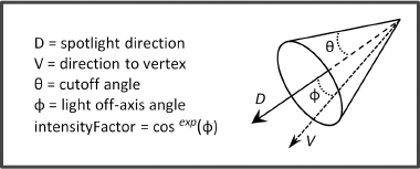
Figure 7.2
Spotlight components.
When designing a system containing many types of lights, a programmer should consider creating a class hierarchy, such as defining a “Light” class and subclasses for “Global Ambient,” “Directional,” “Positional,” and “Spotlight.” Because spotlights share characteristics of both directional and positional lights, it is worth considering utilizing C++’s multiple inheritance capability, and to design a Spotlight class that inherits from both directional and positional light classes. Our examples are sufficiently simple that we omit building such a class hierarchy for lighting in this edition.
7.3MATERIALS
The “look” of the objects in our scene has so far been handled exclusively by color and texture. The addition of lighting allows us to also consider the reflectance characteristics of the surfaces. By that we mean how the object interacts with our ADS lighting model. This can be modeled by considering each object to be “made of” a certain material.
Materials can be simulated in an ADS lighting model by specifying four values, three of which we are already familiar with—ambient, diffuse, and specular RGB colors. The fourth is called shininess, which, as we will see, is used to build an appropriate specular highlight for the intended material. ADS and shininess values have been developed for many different types of common materials. For example, “pewter” can be specified as follows:
float pewterMatAmbient[4] = { .11f, .06f, .11f, 1.0f };
float pewterMatDiffuse[4] = { .43f, .47f, .54f, 1.0f };
float pewterMatSpecular[4] = { .33f, .33f, .52f, 1.0f };
float pewterMatShininess = 9.85f;
ADS RGBA values for a few other materials are given in Figure 7.3 (from [BA16]).
Sometimes other properties are included in the material properties. Transparency is handled in the RGBA specifications in the fourth (or “alpha”) channel, which specifies an opacity; a value of 1.0 represents completely opaque and 0.0 represents completely transparent. For most materials it is simply set to 1.0, although for certain materials a slight transparency plays a role. For example, in Figure 7.3, note that the materials “jade” and “pearl” include a small amount of transparency (values slightly less than 1.0) to add realism.
Emissiveness is also sometimes included in an ADS material specification. This is useful when simulating a material that emits its own light, such as phosphorescent materials.
Figure 7.3
Material ADS coefficients.
When an object is rendered that doesn’t have a texture, it is often desirable to specify material characteristics. For that reason, it will be very convenient to have a few predefined materials available to us. We thus add the following lines of code to our “Utils.cpp” file:
// GOLD material - ambient, diffuse, specular, and shininess
float* Utils::goldAmbient() { static float a[4] = { 0.2473f, 0.1995f, 0.0745f, 1 }; return (float*)a; }
float* Utils::goldDiffuse() { static float a[4] = { 0.7516f, 0.6065f, 0.2265f, 1 }; return (float*)a; }
float* Utils::goldSpecular() { static float a[4] = { 0.6283f, 0.5559f, 0.3661f, 1 }; return (float*)a; }
float Utils::goldShininess() { return 51.2f; }
// SILVER material - ambient, diffuse, specular, and shininess
float* Utils::silverAmbient() { static float a[4] = { 0.1923f, 0.1923f, 0.1923f, 1 }; return (float*)a; }
float* Utils::silverDiffuse() { static float a[4] = { 0.5075f, 0.5075f, 0.5075f, 1 }; return (float*)a; }
float* Utils::silverSpecular() { static float a[4] = { 0.5083f, 0.5083f, 0.5083f, 1 }; return (float*)a; }
float Utils::silverShininess() { return 51.2f; }
// BRONZE material - ambient, diffuse, specular, and shininess
float* Utils::bronzeAmbient() { static float a[4] = { 0.2125f, 0.1275f, 0.0540f, 1 }; return (float*)a; }
float* Utils::bronzeDiffuse() { static float a[4] = { 0.7140f, 0.4284f, 0.1814f, 1 }; return (float*)a; }
float* Utils::bronzeSpecular() { static float a[4] = { 0.3936f, 0.2719f, 0.1667f, 1 }; return (float*)a; }
float Utils::bronzeShininess() { return 25.6f; }
This makes it very easy to specify that an object has, say, a “gold” material, in either the init() function or in the top level declarations, as follows:
float* matAmbient = Utils::goldAmbient();
float* matDiffuse = Util::goldDiffuse();
float* matSpecular = util.goldSpecular();
float matShininess = util.goldShininess();
Note that our code for light and material properties described so far in these sections does not actually perform lighting. It merely provides a way to specify and store desired light and material properties for elements in a scene. We still need to actually compute the lighting ourselves. This is going to require some serious mathematical processing in our shader code. So let’s now dive into the nuts and bolts of implementing ADS lighting in our C++/OpenGL and GLSL graphics programs.
7.4ADS LIGHTING COMPUTATIONS
As we draw our scene, recall that each vertex is transformed so as to simulate a 3D world on a 2D screen. Pixel colors are the result of rasterization as well as texturing and interpolation. We must now incorporate the additional step of adjusting those rasterized pixel colors to effect the lighting and materials in our scene. The basic ADS computation that we need to perform is to determine the reflection intensity (I) for each pixel. This computation takes the following form:

That is, we need to compute and sum the ambient, diffuse, and specular reflection contributions for each pixel, for each light source. This will of course depend on the type of light(s) in our scene and the type of material associated with the rendered model.
Ambient contribution is the simplest. It is the product of the specified ambient light and the specified ambient coefficient of the material:

Keeping in mind that light and material intensities are specified via RGB values, the computation is more precisely:

Diffuse contribution is more complex because it depends on the angle of incidence between the light and the surface. Lambert’s Cosine Law (published in 1760) specifies that the amount of light that reflects from a surface is proportional to the cosine of the light’s angle of incidence. This can be modeled as follows:

As before, the actual computations involve red, green, and blue components.
Determining the angle of incidence θ requires us to (a) find a vector from the pixel being drawn to the light source (or, similarly, a vector opposite the light direction), and (b) find a vector that is normal (perpendicular) to the surface of the object being rendered. Let’s denote these vectors  and
and  respectively, as shown in Figure 7.4:
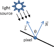
Figure 7.4
Angle of light incidence.
Depending on the nature of the lights in the scene,  could be computed by negating the light direction vector or by computing a vector from the location of the pixel to the location of the light source. Determining vector
  may be trickier—normal vectors may be available for the vertices in the model being rendered, but if the model doesn’t include normals,
  would need to be estimated geometrically based on the locations of neighboring vertices. For the rest of the chapter, we will assume that the model being rendered includes normal vectors for each vertex (this is common in models constructed with modeling tools such as Maya or Blender).
It turns out that in this case, it isn’t necessary to compute θ itself. What we really desire is cos(θ), and recall from Chapter 3 that this can be found using the dot product. Thus, the diffuse contribution can be computed as follows:

The diffuse contribution is only relevant when the surface is exposed to the light, which occurs when -90 < θ < 90; that is, when cos(θ) > 0. Thus, we must replace the rightmost term in the previous equation with:

Specular contribution determines whether the pixel being rendered should be brightened because it is part of a “specular highlight.” It involves not only the angle of incidence of the light source, but also the angle between the reflection of the light on the surface and the viewing angle of the “eye” relative to the object’s surface.
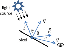
Figure 7.5
View angle incidence.
In Figure 7.5,  represents the direction of reflection of the light, and
  (called the view vector) is a vector from the pixel to the eye. Note that
  is the negative of the vector from the eye to the pixel (in camera space, the eye is at the origin). The smaller the angle φ between
  and
and  , the more the eye is on-axis or “looking into” the reflection, and the more this pixel contributes to the specular highlight (and thus the brighter it should appear).
The manner in which φ is used to compute the specular contribution depends on the desired “shininess” of the object being rendered. Objects that are extremely shiny, such as a mirror, have very small specular highlights—that is, they reflect the incoming light to the eye exactly. Materials that are less shiny have specular highlights that are more “spread out,” and thus more pixels are a part of the highlight.
Shininess is generally modeled with a falloff function that expresses how quickly the specular contribution reduces to zero as the angle φ grows. We can use cos(φ) to model falloff, and increase or decrease the shininess by using powers of the cosine function, such as cos(φ), cos2(φ), cos3(φ), cos10(φ), cos50(φ), and so on, as illustrated in Figure 7.6.
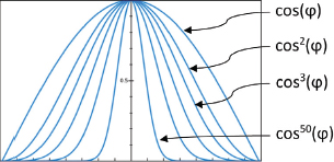
Figure 7.6
Shininess modeled as cosine exponent.
Note that the higher the value of the exponent, the faster the falloff, and thus the smaller the specular contribution of pixels with light reflections that are off-axis from the viewing angle.
We call the exponent n, as used in the cosn(φ) falloff function, the shininess factor for a specified material. Note back in Figure 7.3 that shininess factors for each of the materials listed are specified in the rightmost column.
We now can specify the full specular calculation:

Note that we use the max() function in a similar manner as we did for the diffuse computation. In this case, we need to ensure that the specular contribution does not ever utilize negative values for cos(φ), which could produce strange artifacts such as “darkened” specular highlights.
And of course as before, the actual computations involve red, green, and blue components.
7.5IMPLEMENTING ADS LIGHTING
The computations described in Section 7.4 have so far been mostly theoretical, as they have assumed that we can perform them for every pixel. This is complicated by the fact that normal ( ) vectors are typically available to us only for the vertices that define the models, not for each pixel. Thus, we need to either compute normals for each pixel, which could be time-consuming, or find some way of estimating the values that we need to achieve a sufficient effect.
One approach is called “faceted shading” or “flat shading.” Here we assume that every pixel in each rendered primitive (i.e., polygon or triangle) has the same lighting value. Thus, we need only do the lighting computations for one vertex in each polygon in the model, and then copy those lighting values across the nearby rendered pixels on a per-polygon or per-triangle basis.
Faceted shading is rarely used today, because the resulting images tend to not look very realistic, and because modern hardware makes more accurate computations feasible. An example of a faceted-shaded torus, in which each triangle behaves as a flat reflective surface, is shown in Figure 7.7.
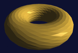
Figure 7.7
Torus with faceted shading.
Although faceted shading can be adequate in some circumstances (or used as a deliberate effect), usually a better approach is “smooth shading,” in which the lighting intensity is computed for each pixel. Smooth shading is feasible because of the parallel processing done on modern graphics cards, and because of the interpolated rendering that takes place in the OpenGL graphics pipeline.
We will examine two popular methods for smooth shading: Gouraud shading and Phong shading.
7.5.1Gouraud Shading
The French computer scientist Henri Gouraud published a smooth shading algorithm in 1971 that has come to be known as Gouraud shading [GO71]. It is particularly well suited to modern graphics cards, because it takes advantage of the automatic interpolated rendering that is available in 3D graphics pipelines such as OpenGL. The process for Gouraud shading is as follows:
1.Determine the color of each vertex, incorporating the lighting computations.
2.Allow those colors to be interpolated across intervening pixels through the normal rasterization process (which will also in effect interpolate the lighting contributions).
In OpenGL, this means that most of the lighting computations will be done in the vertex shader. The fragment shader will simply be a pass-through, so as to reveal the automatically interpolated lighted colors.
Figure 7.8 outlines the strategy we will use to implement our Gouraud shader in OpenGL, for a scene with a torus and one positional light. The strategy is then implemented in Program 7.1.

Figure 7.8
Implementing Gouraud shading.
Program 7.1 Torus with Positional Light and Gouraud Shading
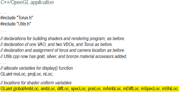
Most of the elements of Program 7.1 should be familiar. The Torus, light, and materials properties are defined. Torus vertices and associated normals are loaded into buffers. The display() function is similar to that in previous programs, except that it also sends the light and material information to the vertex shader. To do this, it calls installLights(), which loads the light viewspace location and the light and material ADS characteristics into corresponding uniform variables to make them available to the shaders. Note that we declared these uniform location variables ahead of time, for performance reasons.
An important detail is that the transformation matrix MV, used to move vertex positions into view space, doesn’t always properly adjust normal vectors into view space. Simply applying the MV matrix to the normals doesn’t guarantee that they will remain perpendicular to the object surface. The correct transformation is the inverse transpose of MV, as described earlier in the supplemental notes to Chapter 3. In Program 7.1, this additional matrix, named “invTrMat”, is sent to the shaders in a uniform variable.
The variable lightPosV contains the light’s position in camera space. We only need to compute this once per frame, so we do it in installLights() (called from display()) rather than in the shader.
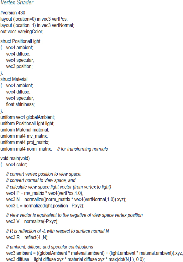
The shaders are shown in the following continuation of program 7.1. The vertex shader utilizes some notations that we haven’t yet seen. Note for example the vector addition done at the end of the vertex shader—vector addition was described in Chapter 3, and is available as shown here in GLSL. We will discuss some of the other notations after presenting the shaders.
The output of Program 7.1 is shown in Figure 7.9.
The vertex shader contains our first example of using the struct notation. A GLSL “struct” is like a datatype; it has a name and a set of fields. When a variable is declared using the name of a struct, it then contains those fields, which are accessed using the “.” notation. For example, variable “light” is declared of type “PositionalLight”, so we can thereafter refer to its fields light.ambient, light.diffuse, and so forth.
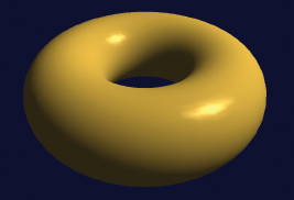
Figure 7.9
Torus with Gouraud shading.
Also note the field selector notation “.xyz”, used in several places in the vertex shader. This is a shortcut for converting a vec4 to an equivalent vec3 containing only its first three elements.
The vertex shader is where most of the lighting computations are performed. For each vertex, the appropriate matrix transforms are applied to the vertex position and associated normal vector, and vectors for light direction ( ) and reflection (
 ) are computed. The ADS computations described in Section 7.4 are then performed, resulting in a color for each vertex (called varyingColor in the code). The colors are interpolated as part of the normal rasterization process. The fragment shader is then a simple pass-through. The lengthy list of uniform variable declarations is also present in the fragment shader (for reasons described earlier in Chapter 4), but none of them are actually used there.
Note the use of the GLSL functions normalize(), which converts a vector to unit length and is necessary for proper application of the dot product, and reflect(), which computes the reflection of one vector about another.
Artifacts are evident in the output torus shown in Figure 7.9. Specular highlights have a blocky, faceted appearance. This artifact is more pronounced if the object is in motion (we can’t illustrate that here).
Gouraud shading is susceptible to other artifacts. If the specular highlight is entirely contained within one of the model’s triangles—that is, if it doesn’t contain at least one of the model vertices—then it may disappear entirely. The specular component is calculated per-vertex, so if a model vertex with a specular contribution does not exist, none of the rasterized pixels will include specular light either.
Bui Tuong Phong developed a smooth shading algorithm while a graduate student at the University of Utah, and described it in his 1973 dissertation [PH73] and published it in [PH75]. The structure of the algorithm is similar to the algorithm for Gouraud shading, except that the lighting computations are done per-pixel rather than per-vertex. Since the lighting computations require a normal vector  and a light vector
  , which are only available in the model on a per-vertex basis, Phong shading is often implemented using a clever “trick,” whereby
  and
and  are computed in the vertex shader and interpolated during rasterization. Figure 7.10 outlines the strategy:

Figure 7.10
Implementing Phong shading.
The C++/OpenGL code is completely unchanged. Some of the computations previously done in the vertex shader are now moved into the fragment shader. The effect of interpolating normal vectors is illustrated in Figure 7.11:
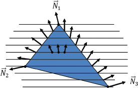
Figure 7.11
Interpolation of normal vectors.
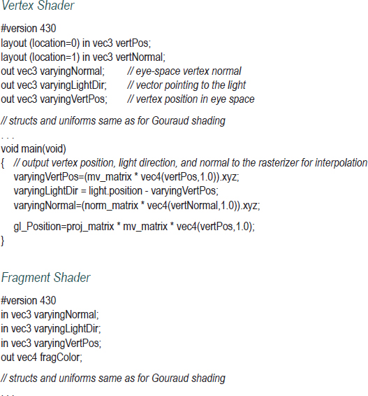
We now are ready to implement our torus with positional lighting, using Phong shading. Most of the code is identical to that used for Gouraud shading. Since the C++/OpenGL code is unchanged, we present only the revised vertex and fragment shaders, shown in Program 7.2. Examining the output of Program 7.2, as shown in Figure 7.12, Phong shading corrects the artifacts present in Gouraud shading.
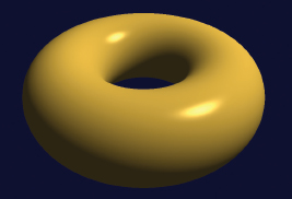
Figure 7.12
Torus with Phong shading.
Program 7.2 Torus with Phong Shading
Although Phong shading offers better realism than Gouraud shading, it does so while incurring a performance cost. One optimization to Phong shading was proposed by James Blinn in 1977 [BL77], and is referred to as the Blinn-Phong reflection model. It is based on the observation that one of the most expensive computations in Phong shading is determining the reflection vector  .
.
Blinn observed that the vector  itself actually is not needed—
 is only produced as a means of determining the angle φ. It turns out that φ can be found without computing
  , by instead computing a vector
  that is halfway between
  and
and  . As shown in Figure 7.13, the angle α between
  and
and  is conveniently equal to ½(φ). Although α isn’t identical to φ, Blinn showed that reasonable results can be obtained by using α instead of φ.
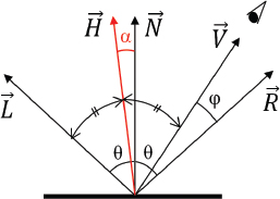
Figure 7.13
Blinn-Phong reflection.
The “halfway” vector  is most easily determined by finding
  +
+  (see Figure 7.14), after which cos(α) can be found using the dot product
  .
.
Figure 7.14
Blinn-Phong computation.
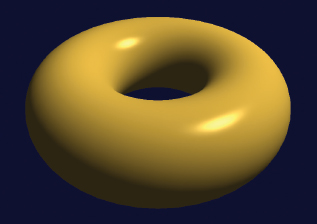
Figure 7.15
Torus with Blinn-Phong shading.
The computations can be done in the fragment shader, or even in the vertex shader (with some tweaks) if necessary for performance. Figure 7.15 shows the torus rendered using Blinn-Phong shading; the quality is largely indistinguishable from Phong shading, with substantial performance cost savings.
Program 7.3 shows the revised vertex and fragment shaders for converting the Phong shading example shown in Program 7.2 to Blinn-Phong shading. As before, there is no change to the C++/OpenGL code.
Program 7.3 Torus with Blinn-Phong Shading
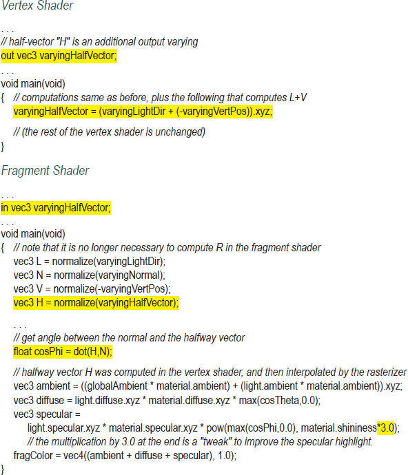
Figure 7.16
External models with Phong shading.
Figure 7.16 shows two examples of the effect of Phong shading on more complex externally generated models. The top image shows a rendering of an OBJ model of a dolphin created by Jay Turberville at Studio 522 Productions [TU16]. The bottom image is a rendering of the well-known “Stanford Dragon,” the result of a 3D scan of an actual figurine, done in 1996 [ST96]. Both models were rendered using the “gold” material we placed in our “Utils.cpp” file. The Stanford dragon is widely used for testing graphics algorithms and hardware because of its size—it contains over 800,000 triangles.
7.6COMBINING LIGHTING AND TEXTURES
So far, our lighting model has assumed that we are using lights with specified ADS values to illuminate objects made of material that has also been defined with ADS values. However, as we saw in Chapter 5, some objects may instead have surfaces defined by texture images. Therefore, we need a way of combining colors retrieved by sampling a texture and colors produced from a lighting model.
The manner in which we combine lighting and textures depends on the nature of the object and the purpose of its texture. There are several scenarios, a few of which include:
•The texture image very closely reflects the actual appearance of the object’s surface.
•The object has both a material and a texture.
•The texture contains shadow or reflection information (covered in Chapters 8 and 9).
•There are multiple lights and/or multiple textures involved.
Let’s consider the first case, where we have a simple textured object and we wish to add lighting to it. One simple way of accomplishing this in the fragment shader is to remove the material specification entirely, and to use the texel color returned from the texture sampler in place of the material ADS values. The following is one such strategy (expressed in pseudocode):
fragColor = textureColor * ( ambientLight + diffuseLight ) + specularLight
Here the texture color contributes to the ambient and diffuse computation, while the specular color is defined entirely by the light. It is common to set the specular contribution solely based on the light color, especially for metallic or “shiny” surfaces. However, some less shiny surfaces, such as cloth or unvarnished wood (and even a few metals, such as gold) have specular highlights that include the color of the object surface. In those cases, a suitable slightly modified strategy would be:
fragColor = textureColor * ( ambientLight + diffuseLight + specularLight )
There are also cases in which an object has an ADS material that is supplemented by a texture image, such as an object made of silver that has a texture that adds some tarnish to the surface. In those situations, the standard ADS model with both light and material, as described in previous sections, can be combined with the texture color using a weighted sum. For example:
textureColor = texture(sampler, texCoord)
lightColor = (ambLight * ambMaterial) + (diffLight * diffMaterial) + specLight
fragColor = 0.5 * textureColor + 0.5 * lightColor
This strategy for combining lighting, materials, and textures can be extended to scenes involving multiple lights and/or multiple textures. For example:
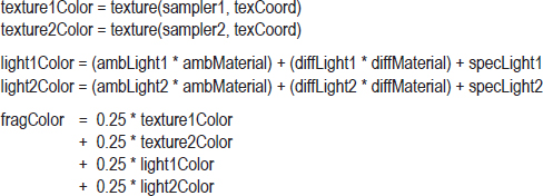
Figure 7.17 shows the Studio 522 Dolphin with a UV-mapped texture image (produced by Jay Turberville [TU16]), and the NASA shuttle model we saw earlier in Chapter 6. Both textured models are enhanced with Blinn-Phong lighting, without the inclusion of materials, and with specular highlights that utilize light only. In both cases, the relevant output color computation in the fragment shader is:

Note that it is possible for the computation that determines fragColor to produce values greater than 1.0. When that happens, OpenGL clamps the computed value to 1.0.
SUPPLEMENTAL NOTES
The faceted-shaded torus shown in Figure 7.7 was created by adding the “flat” interpolation qualifier to the corresponding normal vector vertex attribute declarations in the vertex and fragment shaders. This instructs the rasterizer to not perform interpolation on the specified variable and instead assign the same value for each fragment (by default it chooses the value associated with the first vertex in the triangle). In the Phong shading example, this could be done as follows:
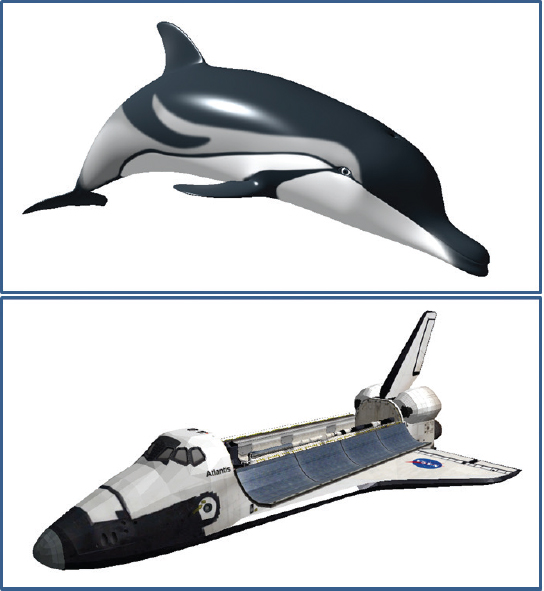
Figure 7.17
Combining lighting and textures.

An important kind of light source that we haven’t discussed is a distributed light or area light, which is a light that is characterized by having a source that occupies an area rather than being a single point location. A real-world example would be a fluorescent tube-style light commonly found in an office or classroom. Interested readers can find more details about area lights in [MH02].
HISTORICAL NOTE
We took the liberty of over-simplifying some of the terminology in this chapter with respect to the contributions of Gouraud and Phong. Gouraud is credited with Gouraud shading—the notion of generating a smoothly curved surface appearance by computing light intensities at vertices and allowing the rasterizer to interpolate these values (sometimes called “smooth shading”). Phong is credited with Phong shading, another form of smooth shading that instead interpolates normals and computes lighting per pixel. Phong is also credited with pioneering the successful incorporation of specular highlights into smooth shading. For this reason, the ADS lighting model, when applied to computer graphics, is often referred to as the Phong Reflection Model. So, our example of Gouraud shading is, more accurately, Gouraud shading with a Phong reflection model. Since Phong’s reflection model has become so ubiquitous in 3D graphics programming, it is common to demonstrate Gouraud shading in the presence of Phong reflection, although it is a bit misleading because Gouraud’s original 1971 work did not, for example, include any specular component.
Exercises
7.1(PROJECT) Modify Program 7.1 so that the light can be positioned by moving the mouse. After doing this, move the mouse around and note the movement of the specular highlight and the appearance of the Gouraud shading artifacts. You may find it convenient to render a point (or small object) at the location of the light source.
7.2Repeat Exercise 7.1, but applied to Program 7.2. This should only require substituting the shaders for Phong shading into your solution to Exercise 7.1. The improvement from Gouraud to Phong shading should be even more apparent here, when the light is being moved around.
7.3(PROJECT) Modify Program 7.2 so that it incorporates TWO positional lights placed in different locations. The fragment shader will need to blend the diffuse and specular contributions of each of the lights. Try using a weighted sum, similar to the one shown in Section 7.6. You can also try simply adding them and clamping the result so it doesn’t exceed the maximum light value.
7.4(RESEARCH AND PROJECT) Replace the positional light in Program 7.2 with a “spot” light as described in Section 7.2. Experiment with the settings for cutoff angle and falloff exponent and observe the effects.
References
[BA16] |
N. Barradeu, accessed October 2018, http://www.barradeau.com/nicoptere/dump/materials.html |
[BL77] |
J. Blinn, “Models of Light Reflection for Computer Synthesized Pictures,” Proceedings of the 4th Annual Conference on Computer Graphics and Interactive Techniques, 1977. |
[DI16] |
Luxo Jr. (Pixar – copyright held by Disney), accessed October 2018, https://www.pixar.com/luxo-jr/#luxo-jr-main |
[GO71] |
H. Gouraud, “Continuous Shading of Curved Surfaces,” IEEE Transactions on Computers C-20, no. 6 (June 1971). |
[MH02] |
T. Akenine-Möller and E. Haines, Real-Time Rendering, 2nd ed. (A. K. Peters, 2002). |
[PH73] |
B. Phong, “Illumination of Computer-Generated Images” (PhD thesis, University of Utah, 1973). |
[PH75] |
B. Phong, “Illumination for Computer Generated Pictures,” Communications of the ACM 18, no. 6 (June 1975): 311–317. |
[ST96] |
Stanford Computer Graphics Laboratory, 1996, accessed October 2018, http://graphics.stanford.edu/data/3Dscanrep/ |
[TU16] |
J. Turberville, Studio 522 Productions, Scottsdale, AZ, www.studio522.com (dolphin model developed 2016). |