SKY AND BACKGROUNDS
The realism in an outdoor 3D scene can often be improved by generating a realistic effect at the horizon. As we look beyond our nearby buildings and trees, we are accustomed to seeing large distant objects such as clouds, mountains, or the sun (or at night, the moon and stars). However, adding such objects to our scene as individual models may come at an unacceptable performance cost. A skybox or skydome provides a relatively simple way of efficiently generating a convincing horizon.
9.1SKYBOXES
The concept of a skybox is a remarkably clever and simple one:
1.Instantiate a cube object.
2.Texture the cube with the desired environment.
3.Position the cube so it surrounds the camera.
We already know how to do all of these steps. There are a few additional details, however.
•How do we make the texture for our horizon?
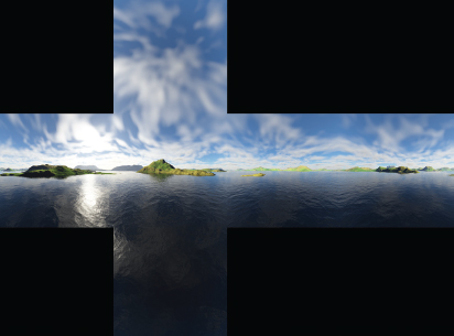
A cube has six faces, and we will need to texture all of them. One way is to use six image files and six texture units. Another common (and efficient) way is to use a single image that contains textures for all six faces, such as shown in Figure 9.1.
Figure 9.1
Six-faced skybox texture cube map.
An image that can texture all six faces of a cube with a single texture unit is an example of a texture cube map. The six portions of the cube map correspond to the top, bottom, front, back, and two sides of the cube. When “wrapped” around the cube, it acts as a horizon for a camera placed inside the cube, as shown in Figure 9.2.
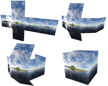
Figure 9.2
Cube map wrapping around the camera.
Texturing the cube with a texture cube map requires specifying appropriate texture coordinates. Figure 9.3 shows the distribution of texture coordinates that are in turn assigned to each of the cube vertices.
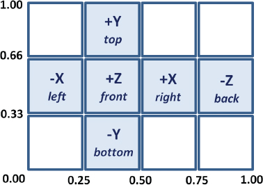
Figure 9.3
Cube map texture coordinates.
•How do we make the skybox appear “distant”?
Another important factor in building a skybox is ensuring that the texture appears as a distant horizon. At first, one might assume this would require making the skybox very large. However, it turns out that this isn’t desirable because it would stretch and distort the texture. Instead, it is possible to make the skybox appear very large (and thus distant), by using the following two-part trick:
 Disable depth testing and render the skybox first (re-enabling depth testing when rendering the other objects in the scene).
Move the skybox with the camera (if the camera moves).
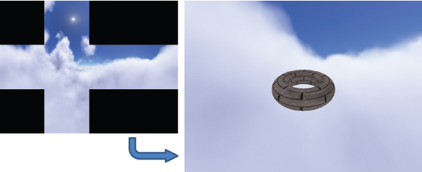
By drawing the skybox first with depth testing disabled, the depth buffer will still be filled completely with 1.0s (i.e., maximally far away). Thus, all other objects in the scene will be fully rendered; that is, none of the other objects will be blocked by the skybox. This causes the walls of the skybox to appear farther away than every other object, regardless of the actual size of the skybox. The actual skybox cube itself can be quite small, as long as it is moved along with the camera whenever the camera moves. Figure 9.4 shows viewing a simple scene (actually just a brick-textured torus) from inside a skybox.
Figure 9.4
Viewing a scene from inside a skybox.
It is instructive to carefully examine Figure 9.4 in relation to the previous Figures 9.2 and 9.3. Note that the portion of the skybox that is visible in the scene is the rightmost section of the cube map. This is because the camera has been placed in the default orientation, facing in the negative Z direction, and is therefore looking at the back of the skybox cube (and so labeled in Figure 9.3). Also note that this back portion of the cube map appears horizontally reversed when rendered in the scene; this is because the “back” portion of the cube map has been folded around the camera and thus appears flipped sideways, as shown in Figure 9.2.
•How do we construct the texture cube map?
Building a texture cube map image, from artwork or photos, requires care to avoid “seams” at the cube face junctions and to create proper perspective so that the skybox will appear realistic and undistorted. Many tools exist for assisting in this regard: Terragen, Autodesk 3ds Max, Blender, and Adobe Photoshop have tools for building or working with cube maps. There are also many websites offering a variety of off-the-shelf cube maps, some for a price, some for free.
9.2SKYDOMES
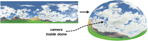
Another way of building a horizon effect is to use a skydome. The basic idea is the same as for a skybox, except that instead of using a textured cube, we use a textured sphere (or half a sphere). As was done for the skybox, we render the skydome first (with depth testing disabled), and keep the camera positioned at the center of the skydome. (The skydome texture in Figure 9.5 was made using Terragen [TE16].)
Figure 9.5
Skydome with camera placed inside.
Skydomes have some advantages over skyboxes. For example, they are less susceptible to distortion and seams (although spherical distortion at the poles must be accounted for in the texture image). One disadvantage of a skydome is that a sphere or dome is a more complex model than a cube, with many more vertices and a potentially varying number of vertices depending on the desired precision.
When using a skydome to represent an outdoor scene, it is usually combined with a ground plane or some sort of terrain. When using a skydome to represent a scene in space, such as a starfield, it is often more practical to use a sphere such as is shown in Figure 9.6 (a dashed line has been added for clarity in visualizing the sphere).

Figure 9.6
Skydome of stars using a sphere (starfield from [BO01]).
Despite the advantages of a skydome, skyboxes are still more common. They also are better supported in OpenGL, which is advantageous when doing environment mapping (covered later in this chapter). For these reasons, we will focus on skybox implementation.
There are two methods of implementing a skybox: building a simple one from scratch, and using the cube map facilities in OpenGL. Each has its advantages, so we will cover them both.
9.3.1Building a Skybox from Scratch
We have already covered almost everything needed to build a simple skybox. A cube model was presented in Chapter 4; we can assign the texture coordinates as shown earlier in this chapter in Figure 9.3. We saw how to read in textures using the SOIL2 library and how to position objects in 3D space. We will see how to easily enable and disable depth testing (it’s a single line of code).
Program 9.1 shows the code organization for our simple skybox, with a scene consisting of just a single textured torus. Texture coordinate assignments and calls to enable/disable depth testing are highlighted.
Program 9.1 Simple Skybox

Standard texturing shaders are now used for all objects in the scene, including the cube map:
The output of Program 9.1 is shown in Figure 9.7, for each of two different cube map textures.
As mentioned earlier, skyboxes are susceptible to image distortion and seams. Seams are lines that are sometimes visible where two texture images meet, such as along the edges of the cube. Figure 9.8 shows an example of a seam in the upper part of the image that is an artifact of running Program 9.1. Avoiding seams requires careful construction of the cube map image and assignment of precise texture coordinates. There exist tools for reducing seams along image edges (such as [GI16]); this topic is outside the scope of this book.
Figure 9.7
Simple skybox results.
9.3.2Using OpenGL Cube Maps
Another way to build a skybox is to use an OpenGL texture cube map. OpenGL cube maps are a bit more complex than the simple approach we saw in the previous section. There are advantages, however, to using OpenGL cube maps, such as seam reduction and support for environment mapping.
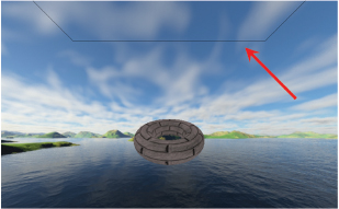
Figure 9.8
Skybox “seam” artifact.
OpenGL texture cube maps are similar to 3D textures that we will study later, in that they are accessed using three texture coordinates—often labeled (s,t,r)—rather than two as we have been doing thus far. Another unique characteristic of OpenGL texture cube maps is that the images in them are oriented with texture coordinate (0,0,0) at the upper left (rather than the usual lower left) of the texture image; this is often a source of confusion.
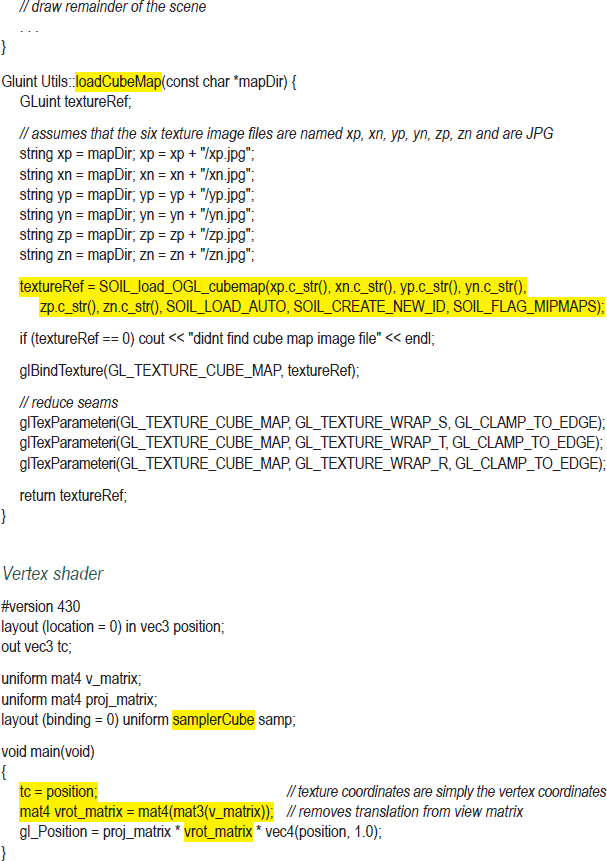
Whereas the method shown in Program 9.1 reads in a single image for texturing the cube map, the loadCubeMap() function shown in Program 9.2 reads in six separate cube face image files. As we learned in Chapter 5, there are many ways to read in texture images; we chose to use the SOIL2 library. Here too, SOIL2 is very convenient for instantiating and loading an OpenGL cube map. We identify the files to read in and then call SOIL_load_OGL_cubemap(). The parameters include the six image files and additional parameters that are similar to the ones for SOIL_load_OGL_texture() that we saw in Chapter 5. In the case of OpenGL cube maps, it isn’t necessary to flip the textures vertically, since OpenGL does that automatically. Note that we have placed loadCubeMap() in our “Utils.cpp” file.
The init() function now includes a call to enable GL_TEXTURE_CUBE_MAP_SEAMLESS, which tells OpenGL to attempt to blend adjoining edges of the cube to reduce or eliminate seams. In display(), the cube’s vertices are sent down the pipeline as before, but this time it is unnecessary to send the cube’s texture coordinates. As we will see, this is because an OpenGL texture cube map usually uses the cube’s vertex positions as its texture coordinates. After disabling depth testing, the cube is drawn. Depth testing is then re-enabled for the rest of the scene.
The completed OpenGL texture cube map is referenced by an int identifier. As was the case for shadow-mapping, artifacts along a border can be reduced by setting the texture wrap mode to “clamp to edge.” In this case it can help further reduce seams. Note that this is set for all three texture coordinates: s, t, and r.
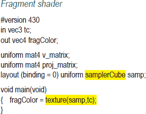
The texture is accessed in the fragment shader with a special type of sampler called a samplerCube. In a texture cube map, the value returned from the sampler is the texel “seen” from the origin as viewed along the direction vector (s,t,r). As a result, we can usually simply use the incoming interpolated vertex positions as the texture coordinates. In the vertex shader, we assign the cube vertex positions into the outgoing texture coordinate attribute so that they will be interpolated when they reach the fragment shader. Note also in the vertex shader that we convert the incoming view matrix to 3x3, and then back to 4x4. This “trick” effectively removes the translation component while retaining the rotation (recall that translation values are found in the fourth column of a transformation matrix). This fixes the cube map at the camera location, while still allowing the synthetic camera to “look around.”
Program 9.2 OpenGL Cube Map Skybox

9.4ENVIRONMENT MAPPING
When we looked at lighting and materials, we considered the “shininess” of objects. However, we never modeled very shiny objects, such as a mirror or something made out of chrome. Such objects don’t just have small specular highlights; they actually reflect their surroundings. When we look at them, we see things in the room, or sometimes even our own reflection. The ADS lighting model doesn’t provide a way of simulating this effect.
Texture cube maps, however, offer a relatively simple way to simulate reflective surfaces—at least partially. The trick is to use the cube map to texture the reflective object itself.1 Doing this so that it appears realistic requires finding texture coordinates that correspond to which part of the surrounding environment we should see reflected in the object from our vantage point.
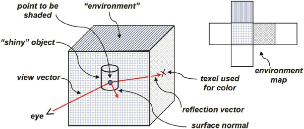
Figure 9.9 illustrates the strategy of using a combination of the view vector and the normal vector to calculate a reflection vector which is then used to look up a texel from the cube map. The reflection vector can thus be used to access the texture cube map directly. When the cube map performs this function, it is referred to as an environment map.
We computed reflection vectors earlier when we studied Blinn-Phong lighting. The concept here is similar, except that now we are using the reflection vector to look up a value from a texture map. This technique is called environment mapping or reflection mapping. If the cube map is implemented using the second method we described (in Section 9.3.2; that is, as an OpenGL GL_TEXTURE_CUBE_MAP), then OpenGL can perform the environment mapping lookup in the same manner as was done for texturing the cube map itself. We use the view vector and the surface normal to compute a reflection of the view vector off the object’s surface. The reflection vector can then be used to sample the texture cube map image directly. The lookup is facilitated by the OpenGL samplerCube; recall from the previous section that the samplerCube is indexed by a view direction vector. The reflection vector is thus well suited for looking up the desired texel.
Figure 9.9
Environment mapping overview.
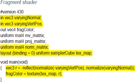
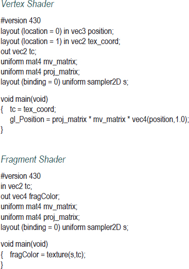
The implementation requires a relatively small amount of additional code. Program 9.3 shows the changes that would be made to the display() and init() functions and the relevant shaders for rendering a “reflective” torus using environment mapping. The changes are highlighted. It is worth noting that if Blinn-Phong lighting is present, many of these additions would likely already be present. The only truly new section of code is in the fragment shader (in the main() method).
In fact, it might at first appear as if the highlighted code in Program 9.3 (i.e., the yellow sections) isn’t really new at all. Indeed, we have seen nearly identical code before, when we studied lighting. However, in this case, the normal and reflection vectors are used for an entirely different purpose. Previously they were used to implement the ADS lighting model. Here they are instead used to compute texture coordinates for environment mapping. We highlighted these lines of code so that the reader can more easily track the use of normals and reflection computations for this new purpose.
The result, showing an environment-mapped “chrome” torus, is shown in Figure 9.10.
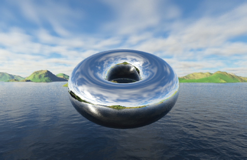
Figure 9.10
Example of environment mapping to create a reflective torus.
Program 9.3 Environment Mapping
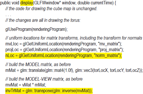
Although two sets of shaders are required for this scene—one set for the cube map and another set for the torus—only the shaders used to draw the torus are shown in Program 9.3. This is because the shaders used for rendering the cube map are unchanged from Program 9.2. The changes made to Program 9.2, resulting in Program 9.3, are summarized as follows:
in init():
•A buffer of normals for the torus is created (actually done in setupVertices(), called by init()).
•The buffer of texture coordinates for the torus is no longer needed.
in display():
•The matrix for transforming normals (dubbed “norm_matrix” in Chapter 7) is created and linked to the associated uniform variable.
•The torus normal buffer is activated.
•The texture cube map is activated as the texture for the torus (rather than the “brick” texture).
in the vertex shader:
•The normal vectors and norm_matrix are added.
•The transformed vertex and normal vector are output in preparation for computing the reflection vector, similar to what was done for lighting and shadows.
•The reflection vector is computed in a similar way to what was done for lighting.
•The output color is retrieved from the texture (now the cube map), with the lookup texture coordinate now being the reflection vector.
The resulting rendering shown in Figure 9.10 is an excellent example of how a simple trick can achieve a powerful illusion. By simply painting the background on an object, we have made the object look “metallic,” when no such ADS material modeling has been done at all. It has also given the appearance that light is reflecting off of the object, even though no ADS lighting whatsoever has been incorporated into the scene. In this example, there even seems to be a specular highlight on the lower left of the torus, because the cube map includes the sunʼs reflection off of the water.
SUPPLEMENTAL NOTES
As was the case in Chapter 5 when we first studied textures, while using SOIL2 makes building and texturing a cube map easy, it can have the unintended conseqence of shielding a user from some OpenGL details that are useful to learn. Of course, it is possible to instantiate and load an OpenGL cube map in the absence of SOIL2. While coverage of this topic is beyond the scope of this book, the basic steps are as follows:
1.Read the six image files (they must be square) using C++ tools.
2.Use glGenTextures() to create a texture for the cube map and its integer reference.
3.Call glBindTexture(), specifying the texture’s ID and GL_TEXTURE_CUBE_MAP.
4.Use glTexStorage2D() to specify the storage requirements for the cube map.
5.Call glTexImage2D() or glTexSubImage2D() to assign the images to cube faces.
For more details on creating OpenGL cube maps in the absence of SOIL2, explore any of the several related tutorials available on the Internet ([dV14], [GE16]).
A major limitation of environment mapping, as presented in this chapter, is that it is only capable of constructing objects that reflect the cube map. Other objects rendered in the scene are not reflected in the reflection-mapped object. Depending on the nature of the scene, this might or might not be acceptable. If other objects are present that must be reflected in a mirror or chrome object, other methods must be used. A common approach utilizes the stencil buffer (mentioned earlier in Chapter 8) and is described in various web tutorials ([OV12], [NE14], and [GR16], for example), but it is outside the scope of this text.
We didn’t include an implementation of skydomes, although they are in some ways arguably simpler than skyboxes and can be less susceptible to distortion. Even environment mapping is simpler—at least the math—but the OpenGL support for cube maps often makes skyboxes more practical.
Of the topics covered in the later sections of this textbook, skyboxes and skydomes are arguably among the simplest conceptually. However, getting them to look convincing can consume a lot of time. We have dealt only briefly with some of the issues that can arise (such as seams), but depending on the texture image files used, other issues can occur, requiring additional repair. This is especially true when the scene is animated, or when the camera can be moved interactively.
We also glossed over the generation of usable and convincing texture cube map images. There are excellent tools for doing this, one of the most popular being Terragen [TE16]. All of the cube maps in this chapter were made by the authors (except for the star field in Figure 9.6) using Terragen.
Exercises
9.1(PROJECT) In Program 9.2, add the ability to move the camera around with the mouse or the keyboard. To do this, you will need to utilize the code you developed earlier in Exercise 4.2 for constructing a view matrix. You’ll also need to assign mouse or keyboard actions to functions that move the camera forward and backward, and functions that rotate the camera on one or more of its axes (you’ll need to write these functions too). After doing this, you should be able to “fly around” in your scene, noting that the skybox always appears to remain at the distant horizon.
9.2Draw labels on the six cube map image files to confirm that the correct orientation is being achieved. For example, you could draw axis labels on the images, such as these:
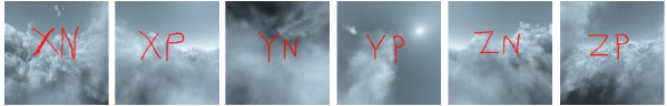
Also use your “labeled” cube map to verify that the reflections in the environment-mapped torus are being rendered correctly.
9.3(PROJECT) Add animation to Program 9.3 so that one (or more) environment-mapped object(s) in the scene rotate or tumble. The simulated reflectivity of the object should be apparent as the skybox texture moves on the object’s surface.
9.4(PROJECT) Modify Program 9.3 so that the object in the scene blends environment-mapping with a texture. Use a weighted sum in the fragment shader, as described in Chapter 7.
9.5(RESEARCH & PROJECT) Learn the basics of how to use Terragen [TE16] to create a simple cube map. This generally entails making a “world” with the desired terrain and atmospheric patterns (in Terragen), and then positioning Terragen’s synthetic camera to save six images representing the views front, back, right, left, top, and bottom. Use your images in Programs 9.2 and 9.3 to see their appearance as cube maps and with environment mapping. The free version of Terragen is quite sufficient for this exercise.
References
[BO01] |
P. Bourke, “Representing Star Fields,” October 2018, accessed July 2016, http://paulbourke.net/miscellaneous/astronomy/ |
[dV14] |
J. de Vries, “Learn OpenGL – Cubemaps,” 2014, accessed October 2018, https://learnopengl.com/Advanced-OpenGL/Cubemaps |
[GE16] |
A. Gerdelan, “Cube Maps: Sky Boxes and Environment Mapping,” 2016, accessed October 2018, http://antongerdelan.net/opengl/cubemaps.html |
GNU Image Manipulation Program, accessed October 2018, http://www.gimp.org | |
[GR16] |
OpenGL Resources, “Planar Reflections and Refractions Using the Stencil Buffer,” accessed October 2018, |
[NE14] |
NeHeProductions, “Clipping and Reflections Using the Stencil Buffer,” 2014, accessed October 2018, |
[OV12] |
A. Overvoorde, “Depth and Stencils,” 2012, accessed October 2018, https://open.gl/depthstencils |
[TE16] |
Terragen, Planetside Software, LLC, accessed October 2018, http://planetside.co.uk/ |
1This same trick is also possible in those cases where a skydome is being used instead of a skybox, by texturing the reflective object with the skydome texture image.