8
The Fracture Criterion of a Laminate
8.1. The sizing criterion
Chapter 5 showed how fracture within a UD ply can be estimated. In the case of a laminate, the problem is slightly more complex because fracture must be evaluated for each ply of the laminate. Further more, in reality, fracture within the first ply rarely leads to the total failure of the laminate which can generally absorb a lot more loading before reaching its limit. We must also keep in mind that a structure will be subjected to different loads throughout its life cycle (and not just one isolated load, which is what we see in academic testing situations) known as “load cases”. An engineer’s duty is then to ensure that the structure will support all of these load cases without breaking and / or straining too much.
In the aeronautical field, the matter is slightly more complicated as we must distinguish between limit loads (LL) and ultimate loads (UL). The sizing of aeronautical structures is indeed highly complex but can be concisely summarized by the statement that the structure must statically support the LL without sustaining damage (and / or plasticity for metallic materials) and the UL without experiencing catastrophic failure [BOU 16, FED 88, JOI 78]. More specifically, the limit load (LL) is defined as the load that the structure will experience on average once in its lifetime, which for the aeronautical industry gives it a probability of occurrence of approximately 10–5 per flight hour (an aircraft flies about 105 hours). As for ultimate load (UL), it is defined as a highly improbable load, which for the aeronautical industry gives it a probability of occurrence of approximately 10–9 per flight hour (ACJ 25.1309 [FED 88]). In practice, there is a coefficient k generally sitting between 1.1 and 1.5 from one to the other:
The sizing philosophy of an aircraft structure can thus be summarized as:
- – No damage or permanent deformation is permitted during service, i.e. under realistic loads or even loads less than or equal to the LL.
- – The structure must remain whole under test loads, i.e. with highly improbable loads or even loads less than or equal to the UL.
We must also add to that any damage problems. The structure, on top of resisting LL and UL, must be able to sustain damages (falling objects, stone impacts, hitting birds, lightning, etc.) without experiencing catastrophic failure. This is the notion of damage tolerance (which we will come back to in the next chapter).
However, no matter the complexity of the structure sizing, it always comes down to demonstrating that the structure (with any potential sustained damage, cracks or missing portions) can withstand such a load without fracturing or overly straining. It therefore needs sizing criteria based on the stress and / or strain fields (or on the strain energy release rate) to demonstrate that the structure can withstand the load. These criteria will obviously need to be verified everywhere in the structure and for all the foreseeable load cases. The engineer’s task will then consist of modifying the design of the structure if that is not the case or if these criteria are not practical (in sum, if the structure is too oversized and thus too heavy).
While the list will never truly be exhaustive, we can attempt to review the different sizing cases of a composite aircraft as follows:
- – Buckling: the laminate will then primarily be sized in terms of bending stiffness. It is very common in the aeronautical field for structures to be made from thin plates designed to withstand compressive loading in particular.
- – Stiffness: the laminate will then be sized in terms of membrane or bending stiffness. We can use the example of space where the primary sizing criterion is often the 1st natural frequency of the system.
- – Damage resistance: the damaged structure must be able to withstand sufficient loads. The most critical damage for composite structure generally tends to be impact and the residual strength after impact criterion is often the most restrictive of all for aircraft structures (see next chapter).
- – Ageing: the resins used in aviation, epoxy for example, degrade over time with exposure to humidity, UV, etc. The structure must therefore be able to withstand loads even after ageing. In practice, this isn’t really a criterion, in the sense that the sizing criterion of the composite remains the same as previously but with the characteristics of the pristine material replacing those of the aged one.
- – Interface fracture: all the calculations performed in this lesson are based on the hypothesis that the laminate remains laminate, in other words that all interfaces are healthy. In reality, there are cases where these interfaces can be damaged, for example on the edges of the plate or when the laminate sustains a small impact, or even from a manufacturing defect such as during a drilling operation. In practice, these cases are complicated to size numerically and global criteria are put in place. These criteria nonetheless remain unfavorable and lead to the composite being used beyond its real capabilities.
8.2. Test on a composite structure
During the certification process of a composite structure in the aeronautical field, a number of experimental tests are required in order to ensure its resistance. If we perform, for example, an experimental test until final fracture, we generally obtain a curve with an initial linear part representing the stiffness of the pristine structure, followed by a nonlinear segment due to various structural damages.
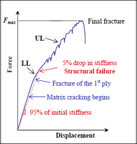
Figure 8.1. Diagram curve of a fracture test on a composite structure. For a color version of this figure, see www.iste.co.uk/bouvet/aeronautical2.zip
Even in the linear portion we can see that there are numerous damages within the structure. Matrix cracks appear in the most loaded areas, but because the stiffness reductions caused by these cracks remain low (most of the stiffness is linked to the fibers) and localized, their effect on the overall stiffness is, generally speaking, practically null.
If we continue to load we then observe the first fiber fractures in certain plies. When these fiber fractures remain localized, their effect on the overall stiffness remains quite low. It is therefore often quite difficult to locate these initial fiber fractures from the force / displacement curve (however they can be heard during a test as fiber fractures are highly energy-concentrated phenomena and can be very loud). In order to characterize these initial fiber fractures, a criterion of overall stiffness reduction is often used. Consider, for example, a stiffness reduction of 5% in the structure (taking the initial stiffness of the structure then multiplying it by 0.95 so that the point of intersection between this line and the real curve will give the desired point; see previous figure). This is then called a “structural fracture”.
If we continue to increase the load, fiber fractures will increase and their effect on the overall stiffness of the structure will become greater and greater. In this portion, we often observe quite violent and noisy fractures (which are quite impressive during the test) that are easily visible on the global force / displacement curve. Lastly, if we increase the load any more, we then obtain the final fracture of the structure (which is very impressive!).
We can now question what LL and UL this structure can support or, in other words, where we can place the LL and UL on this curve (in practice, determining the maximum LL and UL of a structure is almost equivalent to the real problem, which is obviously to design a structure with an awareness of the LL and UL; for example, all it takes is to change the thickness of the plate to lock the maximum LL and UL with the desired ones):
- – The LL are generally placed just before the structural fracture, i.e. just before getting too many fiber fractures. Also keep in mind that no damage or permanent deformation is permitted for loads less than or equal to the LL. We will note, however, that minor damages (in this case, more or less localized matrix cracking) are tolerated, on the condition that they do not reduce the structure’s stiffness too much. In other words, even after minor damages, if you perform another test it should not be noticeable!
- – The UL are located between the LL and the final fracture. It is important not to locate them too close to the final fracture in order to avoid unwanted fracture. It is worth keeping in mind that there is a relatively high variability in composite fracture and variations in the order of 20% of the fracture limit are often encountered.
In the context of this book, we will limit ourselves to predicting the fracture of the first ply and thus establish the LL. If we wish to size a structure to the UL then we will have to take into account ply fracture; we can, for instance, determine the fracture of each ply one after the other, remove their stiffness, and evaluate the stiffness of the structure without them until there are none left. However, sizing to the UL is far more complicated and far surpasses the scope of this book. It has, however, been the subject of many other studies and research [WIS 12, ABD 15, BOU 09, CHA 87, US 97].
8.3. Sizing principle
There are two main cases when sizing a structure:
- – The structure and the loads are known and the objective of the sizing is to demonstrate that it withstands the loads without fracturing and then determine the “reserve factors” (RF). This leads, for example, to applying a Yamada–Sun type fracture criterion to all the plies of the laminate throughout the structure, not forgetting that the laminate plate can hold a large number of plies, that the stacking sequence is not the same throughout the structure, and that the resultant forces and moments vary from one point to the next in the structure.
- – The structure is unknown, and the loads are known. This is the classic case in the aeronautical field where we know the resultant forces that a structure will have to withstand and we are looking to design the lightest possible structure. It is then a matter of determining which stacking sequence to use, which can evidently vary from one point to the next in the structure, in order to withstand the load cases. We can note that not only will the loads depend on the point that is being studied but also on the characteristics of the structure, in other words, of the stacking sequence. We can therefore demonstrate that for a hyperstatic structure (which tends to be the case quite often in reality), the stress distribution depends on the stiffness of a structure. An iterative design process is then necessary in order to optimize the structure.
8.4. Sizing a given structure for a given loading
Consider a composite structure with known geometrical characteristics, in particular its stacking sequence and load cases, which will, in principle, change depending on the given point. The problem can then be reduced to determining the RF, i.e. the safety coefficient, at any given point and in each ply for the loading at that given point.
For a membrane sizing with mirror symmetry, this can be presented as follows:
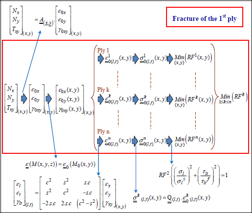
Figure 8.2. Sizing a composite laminate under membrane loading. For a color version of this figure, see www.iste.co.uk/bouvet/aeronautical2.zip
Based on the resultant forces we determine the membrane strain of the midplane and then the strains in each ply (which are obviously homogeneous throughout the thickness since we are studying a membrane loading and plate with mirror symmetry). In practice, these strains will vary in x and y because the stiffnesses vary in the plane of the laminate (if, for example, the number of plies changes) and because the loads vary depending on the position in the structure. We can then determine, for each ply and each point in plane (x, y), the stresses and therefore the RF. We then obtain non-fracture of the first ply if the minimum RF of all the other plies and all the points in the plane (x, y) remain above 1.
For a sizing in bending, the problem is slightly more complicated because we have to add the variation of these strains depending on the thickness:
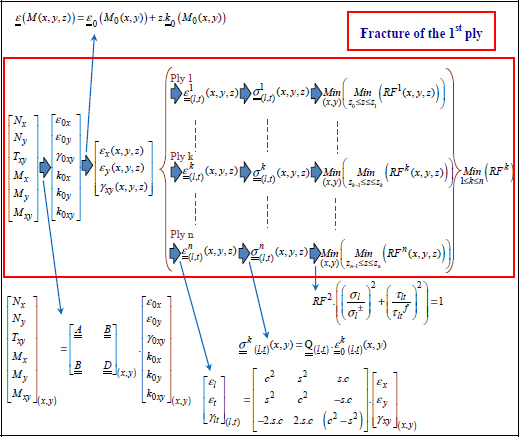
Figure 8.3. Sizing of a composite laminate under bending loading. For a color version of this figure, see www.iste.co.uk/bouvet/aeronautical2.zip
Based on the resultant forces and moments, we determine the membrane strains and curvatures in the midplane and then the strains in the plies that are obviously not homogeneous throughout the thickness. In practice, these strains will vary depending on x and y because the stiffnesses vary in the plane of the laminate (if, for example, the number of plies changes) and because the stresses depend on the position in the structure. We can then determine, in the thickness of each ply and for each point in plane (x, y), the stresses and therefore the RF. We then obtain non-fracture of the first ply if the minimum RF throughout the thickness of all plies and for all points in plane (x, y) remains above 1. In all evidence, for a real problem this work is performed automatically on calculation results by the finite element method.
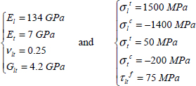
EXAMPLE (Laminate [0, 90]S).– Consider a plate with a thickness h and a stacking sequence [0,90]S composed of UD plies of T300/914, 0.25 mm thick (both 0.125 mm and 0.25 mm standard thicknesses exist) subjected to a resultant force Nx = 400 N/mm. We restate the characteristics of T300/914:
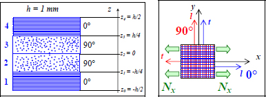
Figure 8.4. Tension of a laminate [0,90]S. For a color version of this figure, see www.iste.co.uk/bouvet/aeronautical2.zip
We begin by calculating the membrane stiffness of the laminate:
We can then determine the strains, which here are homogeneous throughout the thickness of the laminate:
Where we restate that the strains are unit-less and that microstrain (με) is simply a coefficient of 10–6. Thus, for each ply in its axes:
- – For plies 1 and 4 at 0°:
- – For plies 2 and 3 at 90°:
Keeping in mind that frame (l, t) is not the same depending on the direction of the ply.
We can then deduce the stresses which here are homogeneous within each ply:
- – For plies 1 and 4 at 0°:
- – For plies 2 and 3 at 90°:
We then apply a fracture criterion in each ply. We will begin by using the Hill criterion:
- – For plies 1 and 4 at 0°:
- – For plies 2 and 3 at 90°:
Where the RF corresponds to the coefficient by which the load must be multiplied in order to obtain the fracture of the ply:
- – For plies 1 and 4 at 0°: RF = 1.87
- – For plies 2 and 3 at 90°: RF = 1.27
We see that the 1st ply to break will be the one at 90° (for a load equal to 1.27 the set load) and if we trace the respective contribution of each term of the Hill criterion, we note that it breaks under transverse tension. Nonetheless, this premature fracture (compared to the real fracture) under transverse cracking of the 90° ply is not too penalizing for the structure, as long as the plies at 0° are safe. In practice, in order to avoid penalization and not grant too much importance to these secondary matrix cracks, we artificially increase the limit strain of the matrix in the criteria. To do this, we just artificially reduce its Young’s modulus while maintaining the same transverse fracture stress. As an example, by dividing the transverse Young’s modulus by two, we obtain:
And with the Hill criterion:
- – For plies 1 and 4 at 0°: RF = 1.90
- – For plies 2 and 3 at 90°: RF = 2.46
This time, we see that the minimum RF is that of the plies at 0° and the RF for the primary ply, i.e. the one at 0°, has suffered little variation. We can show that the results obtained by reducing Et are then closer to the experimental results in terms of the fracture of the 1st ply. In sum, this method gives us good results by taking into account the influence of the fracture of the plies due to matrix cracking in a more realistic way.
To distance ourselves from this matrix cracking, we can also use the Yamada–Sun criterion. Keeping in mind that we can use this criterion here because there are plies perpendicular to the studied ones (plies at 90° if studying plies at 0°, and vice-versa), we then get:
- – For plies 1 and 4 at 0°: RF = 1.97
- – For plies 2 and 3 at 90°: RF = 156
The RF of plies at 90° is obviously very far from the calculation with the Hill criterion, as the fracture of these plies is primarily due to matrix cracking which is not accounted for in the Yamada–Sun criterion. Nonetheless, this fracture is secondary and is often accepted in real-world applications. Furthermore, it is evidently the weakest RF that will size the structure and therefore, in this case, the one for the plies at 0°, which is close for both the criteria. We can show that this result is representative of the real fracture of the structure.
Lastly, in order to better account for the potential matrix cracks in a real structure, we generally take a modulus Et that is lower than the real modulus of the pristine material. To do this we can, for example, perform a tensile test on a laminate, then identify Et retroactively on the mean modulus Ex of the laminate (the modulus El is then identified directly in a pure UD tensile test). Performing a tensile test with a sufficiently high load will allow the matrix cracking to develop and let us identify the real laminate (with comparable damage in reality). In the case of T300/914 studied here, the value of 7 GPa for Et accounts for these minor damages.
EXAMPLE (Quasi-isotropic laminate [0,45,90,–45]S).– Consider a laminate with a stacking sequence of [0,45,90,–45]S composed of UD plies of 0.125-mm-thick T300/914, subjected to a resultant force Nx = 400 N/mm. Note here that the plies are thinner than in the previous example. This will allow us to achieve the same overall thickness for the laminate, making both the examples easier to compare.
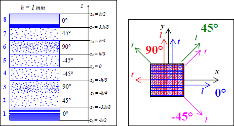
Figure 8.5. Quasi-isotropic laminate [0,45,90,–45]S under tensile loading. For a color version of this figure, see www.iste.co.uk/bouvet/aeronautical2.zip
We begin by calculating the membrane stiffness of the laminate:
We can then determine the strains that, in this case, are evenly distributed in the thickness of the laminate:
We can then deduce the strains in the axes of each ply and the stresses that, in this case, are homogeneous throughout each ply:
- – For plies 1 and 8 at 0°:
- – For plies 2 and 7 at 45°:
- – For plies 3 and 6 at 90°:
- – For plies 4 and 5 at –45°:
Then apply the Yamada–Sun fracture criterion to each ply:
- – For plies 1 and 8 at 0°: RF = 1.41
- – For plies 2 and 7 at 45°: RF = 1.59
- – For plies 3 and 6 at 90°: RF = 4.51
- – For plies 4 and 5 at –45°: RF = 1.59
The RF are higher than 1, meaning that the laminate will withstand the load in question. Of course, since laminates are unsymmetrical in tension / compression, the RF will be different under compression. If, for example, Nx = –400 N/mm, we then get:
- – For plies 1 and 8 at 0°: RF = 1.31
- – For plies 2 and 7 at 45°: RF = 1.57
- – For plies 3 and 6 at 90°: RF = 4.84
- – For plies 4 and 5 at –45°: RF = 1.57
We can then wonder about the maximum load that will cause the final fracture of the laminate (under tension). If we increase Nx, we obtain an RF of 1 in the plies at 0° for Nx = 564 N/mm. The result is obviously equal to the product of the previous RF (RF0° = 1.41) by the corresponding resultant force (Nx = 400 N/mm); this is in fact the very definition of RF (the coefficient by which the load must be multiplied in order to achieve the fracture)!
Similarly, we can trace the RF when the direction of the resultant force Nx = 400 N/mm varies:
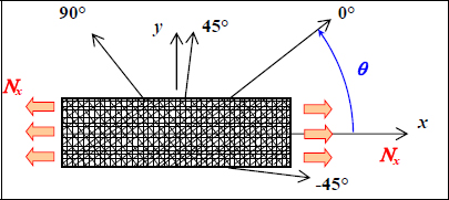
Figure 8.6. Quasi-isotropic laminate [0,45,90,-45]S under off-axis tension. For a color version of this figure, see www.iste.co.uk/bouvet/aeronautical2.zip
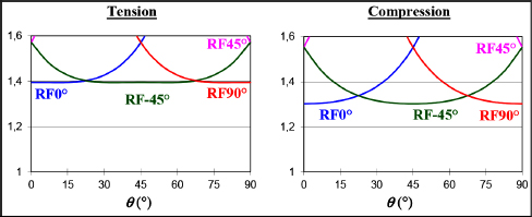
Figure 8.7. RF under off-axis tension and compression of a quasi-isotropic laminate [0,45,90,–45]S. For a color version of this figure, see www.iste.co.uk/bouvet/aeronautical2.zip
And we then observe that the minimum RF (which is obviously the size-determining factor) is practically isotropic both under tension and under compression. In practice, it varies between 1.3 and 1.4 depending on the orientation.
This stacking sequence, known as quasi-isotropic, is therefore practically isotropic (as its name would indicate) in the characteristics of the fracture of its 1st ply.
In sum, the quasi-isotropic stacking sequence is isotropic in its membrane stiffness, quasi-isotropic as far as its resistance to fracture under membrane loading, but non-isotropic in both its bending stiffness and its characteristics of fracture under bending (I’ll leave the demonstration to you).
EXAMPLE (Laminate [0, 90]S).– Consider a laminate with a stacking sequence [0,90]S composed of 0.25-mm-thick UD plies of T300/914 subjected to a resultant moment Mx = 100 N.
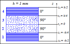
Figure 8.8. Laminate [0,90]S. For a color version of this figure, see www.iste.co.uk/bouvet/aeronautical2.zip
We begin by calculating the bending stiffness of the laminate:
We can then determine the strains and curvatures of the midplane (the strains are obviously not homogeneous throughout the laminate’s thickness):
Then:

Figure 8.9. Strains within the plies of a laminate [0,90]S under bending resultant moment Mx. For a color version of this figure, see www.iste.co.uk/bouvet/aeronautical2.zip
Thus, the maximum strains and stresses in each ply:
- – For ply 1 at 0°: maximum (in absolute value) at z = –h/2
- – For ply 2 at 90°: maximum (in absolute value) at z = –h/4
- – For ply 3 at 90°: maximum (in absolute value) at z = h/4
- – For ply 4 at 0°: maximum (in absolute value) at z = h/2
We then apply the Yamada–Sun fracture criterion to each ply:
- – For ply 1 at 0°: RF = 2.06
- – For ply 2 at 90°: RF = 69.4
- – For ply 3 at 90°: RF = 64.8
- – For ply 4 at 0°: RF = 2.20
We see that evidently the most loaded plies are the ones at 0° since they are the ones that provide bending stiffness and will support most of the loading. We also note that ply 1 is more loaded than ply 4, as its stress mainly comes from compression along the l-direction and that the stress limit under compression is lower than under tension.
The method presented in this section therefore allows us to relatively easily estimate the RF of a laminate for a given load. Obviously, the calculations quickly become tiresome when done by hand and are generally performed with the use of numerical tools. For example, a calculation code using finite element method will provide us with the RF for every ply within a structure, allowing us to redesign the said structure so as to optimize the RF closest to and above 1, while minimizing its mass. Obviously, each modification to the structure will require new calculations, which can be costly in terms of calculation and analysis time. And some analytical optimization methods for the stacking sequence, such as the one we will see in the next section, can help save time by leading us to an initial relevant solution, which can then be optimized using finite element tools.
8.5. Optimal structure for a given load
In many cases, the first stages of design will determine the shape of the structure and the loads it will have to support. The problem then becomes deciding on a material and a stacking sequence in order to support the load while having a minimal mass. The choice of material is generally intricately tied to the cost and its specific characteristics, which is something we will not delve into here. So the last thing to do is to determine the stacking sequence everywhere in the structure as it must vary gradually from one area to the next so as to avoid overstressing due to sudden changes in the stiffness and the complex manufacturing. Over a given area, the stacking sequence will therefore be constant and the problem is then determining the stacking sequence for the point of highest stress while minimizing its mass.
For a membrane optimization with mirror symmetry, this can be summed up as:
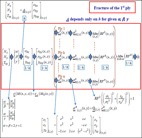
Figure 8.10. Optimization of a laminate for a given load under membrane loading. For a color version of this figure, see www.iste.co.uk/bouvet/aeronautical2.zip
From the resultant force, we determine the ratio of the ply in each direction from the ratio of the stress in that direction. If we name:
- – α the fiber ratio at 0°;
- – β the fiber ratio at 90°;
- – γ the fiber ratio at 45°;
- – γ the fiber ratio at –45°;
supposing, of course, that the fiber ratio at 45° is equal to that at –45°. The fibers at ±45° are used to support shear stress which then decomposes into tensile stress at +45° and compressive stress at –45°; the fiber ratio in these two directions must in principle be the same. We will note, however, that composite materials tend to be more resistant to tension than they are to compression. We can afford to place fewer fibers at +45° than at –45° if shear loading remains constantly positive.

Figure 8.11. Equivalence between shearing and tension / compression at 45°. For a color version of this figure, see www.iste.co.uk/bouvet/aeronautical2.zip
We obviously get the sum of the fiber ratios equal to 1:
Then:
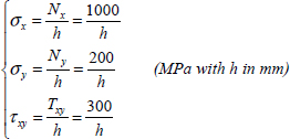
Where Nx, Ny and Txy are the resultant forces that must be supported. We can then determine the fiber ratio in each direction.
Lastly, in reality, loads will tend to vary throughout the life cycle of a structure depending on its complexity and, in order to circumvent certain unexpected loads, it is often expected to place at least 10% of the plies in each direction, 0°, 45°, 90° and –45°. Having a minimum number of plies in each direction also allows them to support loads near holes or rivets. In these areas that receive a lot of stress, even if the average loading is simple, the presence of holes creates complex localized stress fields with all the components of the resultant forces. Setting a minimum of 10% of plies in every direction allows these secondary loads to not be treated and instead bear a couple of maximum loads. If we didn’t have plies in one direction, even a case involving a load causing low levels of stress could prove to be critical.
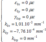
We can then determine the stiffness matrix of the laminate, which will be linear in h, then the strain, which will vary in 1/h. Obviously, the strain can vary along x- and y-directions, because the stress varies according to the location in the structure. We can then determine, in each ply and for each point in the plane (x, y), the stress and the RF that will vary in 1/h. We then obtain non-fracture of the 1st ply by dictating that the minimum RF of all the plies and for all the points in the plane (x, y) be equal to 1. We then get the value of h and thus the stacking sequence (Figure 8.10).
For an optimization under bending loading, the problem is more complicated because the variations in strain depending on the thickness must be included. Subsequently, there isn’t really any usable technique other than experience and the previous solutions:
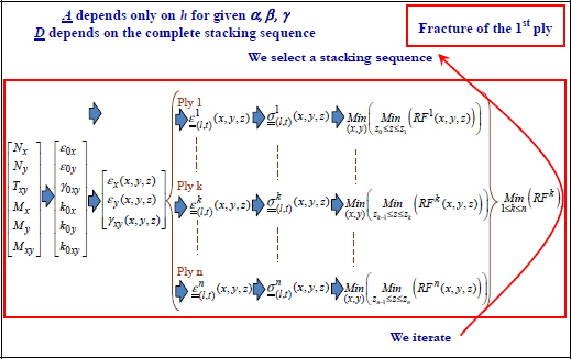
Figure 8.12. Optimization of a laminate for a given bending loading. For a color version of this figure, see www.iste.co.uk/bouvet/aeronautical2.zip
In evidence, the trick is to iterate by starting with a stacking sequence, checking that all the RF remain higher than 1 and then, depending on the result, increasing or reducing the number of plies.
EXAMPLE (Let us determine the optimal stacking sequence for) .–
According to equations [8.24] and [8.25], we get:
We maintain the minimum of 10% in each direction. We then determine the membrane stiffness of the laminate, which is linear in h:
Thus, for the strains that here are homogeneous throughout the thickness of the laminate:
Thus:
- – For plies at 0°:
- – For plies at 90°:
- – For plies at 45°:
- – For plies at –45°:
We then apply the Yamada–Sun fracture criterion to each ply:
- – For plies at 0°: 1.52/h ≤ 1
- – For plies at 90°: 1.18/h ≤ 1
- – For plies at 45°: 1.59/h ≤ 1
- – For plies at –45°: 0.61/h ≤ 1
We take the maximum value of h for all the four directions, i.e.:
Taking thirteen 0.125 mm-thick plies:
- – 7 plies at 0°, i.e.: α = 55%
- – 2 plies at 90°, i.e.: β = 15%
- – 2 plies at 45°, i.e.: γ = 15%
- – 2 plies at –45°, i.e.: γ = 15%
Note that to respect mirror symmetry, you necessarily need even numbers of plies at ±45° and one of the two numbers of plies at 0° and 90° to be even. Evidentally, only the number of plies at 0° or (mutually exclusively) at 90° can be uneven. In fact, it is this uneven ply that will be at the center of the stacking sequence and the midplane of the laminate will be the center of this ply.
We then get the following RF:
- – For plies at 0°: RF = 1.01
- – For plies at 90°: RF = 1.29
- – For plies at 45°: RF = 0.97
- – For plies at –45°: RF = 2.46
We then obtain a RF below 1 for plies at 45°: this is due to not respecting the exact ratios of the plies in each direction. The number of plies being integer, the calculated ratios cannot exactly be respected. And indeed, if we redo the previous test, we get a Yamada–Sun criterion for the most critical ply, the one at 45°, of:
It is then just a matter of adding, for example, a ply at 0°. We could also have added a ply at 45° but that would have forced us to add two plies at 45° and two plies at –45° to respect the mirror symmetry and have a balanced stacking sequence (as many plies at +45° and at –45°):
- – 8 plies at 0°: RF = 1.07
- – 2 plies at 90°: RF = 1.32
- – 2 plies at 45°: RF = 1.03
- – 2 plies at –45°: RF = 2.67
And this time the RF are all higher than 1. We can, for instance, use a stacking sequence:

Which will mean that for a T300/914 with a density of 1,600 kg/m3, we obtain an area density of 2.8 kg/m2. We can then compare this mass to that of a standard aeronautical aluminum alloy (type 2024):
This material being isotropic, we get:
Then writing the Von Mises criterion for in-plane stress state:
Thus:
And:
Meaning, for a density of aluminum alloy of 2,700 kg/m3, an area density of 7.4 kg/m2.
We then get a structure 2.6 times as light in composite. This result should nonetheless be nuanced with other criteria such as buckling resistance, hole and bolt sizing, tolerance to impact damage, etc.

