15
Solutions to the Exercises
15.1. Experimental determination of the characteristics of a UD material

Figure 15.1. Tensile tests for the characterization of a UD ply. For a color version of this figure, see www.iste.co.uk/bouvet/aeronautical2.zip
Question 1
The tabs are necessary in order to minimize the stress concentration in the grips of the testing machine. They are particularly important when we are looking for the fracture limits. In sum, if we simply tighten the specimen alone, we would quickly obtain a fracture at the grip edge, and the maximum stress would therefore be far lower than the real fracture limit!
Question 2
The elastic behavior law of a UD ply is characterized by the two Young’s moduli El and Et, by the Poisson coefficient νlt and the shear modulus Glt; the relation between the stress and strain is:

Evidently, this relation is only true in the frame (l, t)!
In the case of the test at 0°, the frame (x, y) is also the frame (l, t); we therefore get:

Thus:

And:

The test at 90° then allows us to determine the Young’s modulus Et and:

Thus:

And:

The test at 20° allows us to determine the shear modulus. We must begin by determining the stress tensor in the frame (l, t) by performing the rotation from (x, y) to (l, t):

With c = cosθ and s = sinθ. Thus:

And then all that is left to do is put the strain tensor back into the frame (x, y) performing a rotation of −θ (just change s to –s, and do not forget coefficients 2 as a result of the famous εxy = γxy/2):

Knowing that only component εx is what we are interested in:

Thus:

Question 3
In the case of the tensile test at 0°, the frame (x, y) is evidently the principal frame; thus:

As in the case of tension at 90°:

You can also choose xII = −x if you want; then (xI, xII) is a direct orthonormal frame. In practice, only the directions of xI and xII are of any interest to us.
Obviously, the problem is slightly more complicated in the case of tension at 20°. We of course have:

However, this frame is not the principal frame for the strain; indeed, γxy is not null:

This is due to the fact that the material is orthotropic and is loaded outside of its orthotropic axes. The principal stress and strain frames are therefore different.
To determine the principal strains, it should be written:

Remembering to write the strains in the form of a matrix:

as the vector notation is practical, but is mathematically incorrect, and this pseudo-vector does not have the properties of a real vector. This equation (equation [15.17]) has two solutions, the principal strains:

All that remains is to determine the principal directions using:

Thus for example:

Noting at the same time that the two principal directions are of course perpendicular, and that these vectors are defined within a multiplication coefficient (in sum only the direction is important), and in particular that the vector units have no significance. Thus, the following illustration:

Figure 15.2. Position of the principal strain frame. For a color version of this figure, see www.iste.co.uk/bouvet/aeronautical2.zip
Question 4
The Hill criterion is defined by:

with:

Keeping in mind that this relation is true only in frame (l, t)!
In the case of tension at 0°, we obtain:

The Hill criterion can be summed up as:

Thus, the fracture:

In the case of tension at 90°, we have:

The Hill criterion can be summarized as:

Thus, the fracture:

And in the case of tension at 20°, we have:

The Hill criterion leads to:

Which allows us to determine τltf:

We note that in practice, we would avoid using an off-axis tensile test to determine the shear stress limit τltf, as this type of test has a tendency to underestimate τltf. Instead, a rail shear test would be more appropriate [BER 99, GAY 97], though this test is harder to perform.
Question 5
To completely determine the Hill criterion, we are missing the two compression characteristics, σlc and σtc. To obtain these, the simplest approach is to perform a compression test at 0° and one at 90°. In order to correctly introduce the stress into the specimen, we will often use aluminum tabs onto which the composite specimen is glued:

Figure 15.3. Compression test [ABI 08]. For a color version of this figure, see www.iste.co.uk/bouvet/aeronautical2.zip
15.2. Fracture of a laminate
Question 1
To determine if the laminate [45, −45, 02, 90, 0]S will break when subjected to a tensile resultant force of Nx = 2,500 N/mm, we must first determine the stresses within each ply, then apply a fracture criterion such as the Hill criterion. To achieve this, we must begin by determining A, the stiffness matrix of the laminate. Then, we can determine the membrane strains of the plate (these strains are homogeneous throughout the thickness, because the laminate presents mirror symmetry and is subject to membrane loading). The next step is to determine the strains within the frame (l, t) of each ply, then the stresses within the frame (l, t) of each ply, and then apply the fracture criterion (or determine the corresponding RF, which is essentially the same thing) (Figure 8.2).
We therefore start by calculating the matrix  via the stiffness matrix Qijk of each ply (making sure to write these stiffness matrices in the frame (x, y), otherwise you cannot sum them up so simply):

Since we are dealing with membrane forces and the laminate presents a mirror symmetry, the order of the plies is unimportant, and we can regroup the plies in the same orientation:

After using the matrices Qijk in the frame (x, y):

We note that A16 and A26 are null since there are as many plies at +45° as there are at −45°, and that A11 is higher than A22 since there are more plies at 0° than there are at 90°.
We can then determine the strains:

The next step is to place all these strains in the frame (l, t) of each ply, then determine the stresses (since we are now in the frame (l, t) of each ply, the stiffness matrix Qijk is the same for all the plies):
- – For plies at 0°:

- – For plies at 90°:

- – For plies at +45°:

- – For plies at −45°:

We can then determine the RF for each ply, meaning the coefficient by which we must multiply the load to achieve fracture:

This gives us:
- – For plies at 0°: RF = 1.62
- – For plies at 90°: RF = 0.82
- – For plies at +45°: RF = 1.18
- – For plies at −45°: RF = 1.18
The minimum of the RF is therefore 0.82, and the fracture of the laminate is achieved for Nx = 2,500 N/mm in the plies at 90°. We will see further along that this fracture is largely exaggerated!
Question 2
By definition of the RF, we obtain laminate fracture for:

And more specifically, we obtain the fracture of plies at 90° when Nx = Nxt.
Question 3
In reality, this laminate breaks for a much higher resultant force than the one presented in the previous question. This is due to the fact that the fracture of the plies at 90° will not lead to the total failure of the laminate, but rather will induce matrix cracking in the plies at 90°. In order to avoid granting too much importance to these matrix cracks, we must modify the considered fracture criterion. For example, we must remove the part that is due to the transverse stress in the Hill criterion, which is essentially the same as using the Yamada–Sun criterion:

We then get:
- – For plies at 0°: RF = 1.62
- – For plies at 90°: RF = 2.92
- – For plies at +45°: RF = 1.61
- – For plies at −45°: RF = 1.61
And the fracture resultant force is therefore:

Which is relatively close to the experimental value.
The drawback with this type of criterion is that it slightly overvalues the stiffness of the material and does not account for matrix cracks. Once the plies at 90° break (and at ±45°, as we will see later on), the lowered level of modulus Et on the overall stiffness of the laminate should also be accounted for. In order to include this reduced stiffness, we can progressively remove transverse stiffness in the plies experiencing matrix cracking (keeping in mind that even with matrix cracks, a ply can continue to operate, on the condition that it is stabilized by a perpendicular ply).
We can then begin to use Et = 0 MPa for the plies at 90°. We then obtain:

We will note at this point that matrix has but slightly changed in comparison with the previous case; this makes sense since most of the stiffness is provided by the fibers.
We can then determine the membrane strains in the laminate:

Then the strains and stresses within each ply:
- – For plies at 0°:

- – For plies at 90°:

- – For plies at +45°:
- – For plies at −45°:

The primary difference is obviously the stress σt in the plies at 90° that is null (because Et is null!).
Thus, the RF with the Hill criterion:
- – For plies at 0°: RF = 1.60
- – For plies at 90°: RF = 2.82
- – For plies at +45°: RF = 1.16
- – For plies at −45°: RF = 1.16
Which gives us a fracture resultant force:

which is still too low in comparison with the reality. The plies at ±45° are now the ones to break under matrix cracking, and if we decrease Et in these plies, we then find the RF using the Hill criterion:
- – For plies at 0°: RF = 1.61
- – For plies at 90°: RF = 1.61
- – For plies at +45°: RF = 1.61
- – For plies at −45°: RF = 2.84
And we find the same fracture resultant force as with the Yamada–Sun criterion, which remains coherent with the experimental results:

We can then compare the equivalent moduli for the pristine laminate:

with those for the laminate where the Et modulus of plies at 0° and ±45° have been decreased:

We note that the stiffnesses are close due to the fact that they are primarily due to the fibers.
In practice, you should avoid using a criterion that grants too much importance to matrix cracking, such as the Hill criterion, at the risk of oversizing your structure. We can also gradually take into account the matrix cracking, by gradually decreasing the transverse Young’s modulus of the plies broken under matrix cracking. This approach is similar to the use of a fracture criterion that does not account for matrix cracking such as Yamada–Sun’s, but can slightly overestimate the overall stiffness of the laminate (even if in reality, since the modulus Et is assessed from tests that would induce matrix cracking, the experimental value already includes part of this damage).
Question 4
To determine the fracture resultant force under compression, simply use the approach we detailed above, making sure to use the correct stress limit value following the sign of σl, which here will give you, for a resultant force Nx = −2,500 N/mm (and a Yamada–Sun criterion):
- – For plies at 0°: RF = 0.84
- – For plies at 90°: RF = 5.60
- – For plies at +45°: RF = 1.39
- – For plies at −45°: RF = 1.39
Which gives us a fracture resultant force:

We note here that the 1st ply to break is the one at 0°, and it breaks for a value lower than under tension. This is due to the fact that the stress limit under longitudinal compression (−1,200 MPa) is far lower (in absolute value) than that under tension (2,300 MPa). The fiber fracture under compression is indeed guided by the buckling of fibers (and thus by the shear resistance of the resin; see Chapter 4) while the fiber fracture under tension is guided by the tensile fracture of fibers. This explains in particular that newer composite materials have better tensile stress limits than the 1st generation did, while the compressive stress limits remain similar.
15.3. Shear modulus
Question 1
We must begin by remembering how the shear modulus is defined. Imagine holding this material in your hands without knowing that it is a UD ply at 45°. You would then have defined its stiffness matrix  or its compliance matrix
  (the compliance matrix highlights the Young’s and shear moduli more simply than the stiffness matrix) by:

You can then determine Gxy as follows:
- – start by imposing a stress tensor in (x, y) of which only τxy is non-zero;
- – then determine the stress tensor in (l, t);
- – determine the strains in (l, t) using the compliance matrix;
- – perform the inverse rotation to determine the strains in (x, y);
- – you can then identify Gxy as the term linking γxy and τxy.
However, you can also use the laminate membrane stiffness matrix . I will let you verify that both the methods produce the same results. The membrane stiffness matrix , or more specifically its inverse, compliance matrix −1, can be related to the previous compliance matrix. Indeed, we obtain:

The subscript 0 on the strains means that the strains are homogeneous throughout the thickness, which here is the case, because the laminate (in this case, a UD ply at 45°) presents mirror symmetry and is loaded only with membrane force.
We must now link the stresses and resultant forces. In this case, the stresses are homogeneous in the thickness; we just need to multiply it by the thickness. In the case of a real laminate (with multiple plies in different orientations), the resultant forces are tied to the average stress (thus the subscript 0 in the following equation) by:

Keeping in mind that the average stresses are simply the averages of the stresses and are therefore never supported by the material. In particular, applying a fracture criterion to these average stresses makes no sense.
Lastly, we can identify the compliance matrix of the laminate, multiplied by the thickness:

We should begin by determining the stiffness matrix of the laminate:

Where h must be expressed in mm so that is in N/mm. Thickness h is unknown, and we can evidently demonstrate that the shear modulus Gxy does not depend on h. Indeed, if we invert matrix and multiply the result by h, the dependence on h disappears:

This way, we can determine the elastic characteristics of the laminate (in this case, a UD ply at 45°):

Obviously, you will note that the coupling coefficients ηx and ηy are non-zero; meaning that there is coupling between tension and shear.
Question 2
We can use the same approach as previously with the fabric ply. We then obtain:

Then:

Then identifying the elastic characteristics of the laminate (in this case a ply of fabric at 45°):

We of course observe a shear modulus that is much higher than previously (25.7 GPa against 6.4 GPa for the UD)! A shear stress being equal to a tensile stress at +45° and a compressive stress at −45°; to properly support this stress, we need to place fibers at +45° and at −45° (which is not the case with a UD ply at +45°).
We also observe that the coupling coefficients are low. They would be null if there were as many fibers at +45° as there are at −45°. Here, this is practically the case; there are in fact as many fibers in both the directions of the fabric, but since the stiffness in the warp direction is slightly higher than in the weft direction, we create a small imbalance between both the orientations.

Figure 15.4. Example of a fabric ply (satin 8HS). For a color version of this figure, see www.iste.co.uk/bouvet/aeronautical2.zip
15.4. Optimization of stacking sequence
Question 1
To determine an optimal stacking sequence for a given load, we follow the procedure presented in Figure 8.10. We begin by determining the ply ratio in each direction (α at 0°, β at 90 and γ at ±45°) supposing, initially, that they are proportional to the amount of stress:

Furthermore, we note that as Txy = 0, we should find γ = 0. However, we cannot guarantee that during the life cycle of the structure, there will never be a shear resultant force; therefore, we include a minimum of 10% of plies in each direction (see Chapter 13). Thus:

Question 2
Supposing that we know the thickness h of the laminate, we can then determine the ply thickness in each direction:

We then determine the membrane stiffness of the laminate, which is linear in h:

Thus the strains, which in this case are homogeneous in the thickness of the laminate:

Thus:
- – For plies at 0°:

- – For plies at 90°:

- – For plies at +45°:

- – For plies at −45°:

We then apply the Yamada–Sun fracture criterion to each ply:
- – For plies at 0°: 1.67/h ≤ 1
- – For plies at 90°: 1.56/h ≤ 1
- – For plies at +45°: 1.97/h ≤ 1
- – For plies at −45°: 1.97/h ≤ 1
We of course take the maximum values for h for all four directions, i.e.:

Therefore, 16 plies of 0.125 mm thickness. Taking care to use an even number of plies at ±45° so as to maintain mirror symmetry, and an even number of plies at 0° or at 90° (one of the two can be odd, but not both), we obtain, for example:
- – 6 plies at 0°, therefore: 38%
- – 6 plies at 90°, therefore: 38%
- – 2 plies at 45°, therefore: 12%
- – 2 plies at −45°, therefore: 12%
We must then recheck the RF in each ply, indeed except for certain cases, we cannot respect the exact ply ratio in each direction (in the present case, we are very close to it), which will then give us:
- – For plies at 0°: RF = 1.14
- – For plies at 90°: RF = 1.22
- – For plies at 45°: RF = 0.96
- – For plies at −45°: RF = 0.96
We must therefore increase the number of plies, for example, by adding a ply at 0°:
- – For plies at 0°: RF = 1.29
- – For plies at 90°: RF = 1.24
- – For plies at 45°: RF = 1.03
- – For plies at −45°: RF = 1.03
We can for example take a stacking sequence of 17 plies [45, −45, 0, 90, 0, 90, 0, 90, 00.5]S (where the 0.5 factor means that with symmetry, we only have one ply at 0° in the center).
Question 3
To determine the buckling limit, we begin by determining the bending matrix by:

We then find for a stacking sequence [45, −45, 0, 90, 0, 90, 0, 90, 00.5]S:

Thus:

And

This value is much lower to the resultant force −1,000 N/mm along x-direction used to size this stacking sequence against failure. This result is typical; we indeed note that a panel under compression is generally more sensitive to buckling than to compression, and it is its buckling resistance that governs its stacking sequence and in particular its thickness. In the present case, we can make an initial estimate of the thickness required to hold under buckling along x-direction, noting that the buckling resistance evolves with the cube of the thickness, thus the necessary thickness:

Upon 1st approximation, we would need to multiply the thickness by 2.8 to resist buckling along x-direction. For more details, see exercise 8.
Also note at this point that the tension along y-direction will limit buckling, but that the analytical calculation becomes more delicate and goes beyond the scope of the present book. Readers who are interested in finding out more can refer to [BER 99, US 97].
15.5. Composite tube
- – Tension: F = F.x in A with F > 0
In the case where the tube is subject to tensile loading, we had obviously better place all the fibers at 0°, unless we are adhering to the 10% of fibers in each direction rule. In this case, in order to avoid unpredicted loading to other directions, we will use, for instance, 10% of fibers at 90°, 10% at +45°, 10% at −45° and 70% at 0°. In reality, we can still create this tube using only plies at 0°, but on the condition that it is protected. For example, we could place all the plies at 0°, then cover it with fabric to protect it and absorb loading other than the primary tension (for example, impacts resulting from falling objects during manufacturing, maintenance or in operation).

Figure 15.5. Composite tube under tension/compression/torsion/bending. For a color version of this figure, see www.iste.co.uk/bouvet/aeronautical2.zip
In practice, the composite tubes are often made by the filament winding technique. We cover a mandrel with a composite wire (or with a strand of fibers that has been impregnated with resin, to be precise) or a small strip of prepreg. It is then just a matter of controlling the rotation speed of the tube and the movement of the wire to obtain different orientations. This allows us to achieve angles other than the traditional 0°, 90° and ±45° (see exercise 9). The drawback is that the 0° orientation is practically impossible to achieve, and we will use orientations of a few degrees minimum.
Once the stacking sequence has been determined, all that is left to do is use the Hill criterion to determine the thickness of the laminate, knowing the tensile resultant force Nx which is simply determined by (we divide the loading by the length of the plate in question):


Figure 15.6. Composite tube under tension. For a color version of this figure, see www.iste.co.uk/bouvet/aeronautical2.zip
This result is obviously equivalent to the most classic calculation of tensile stress:

Note that in this formula, it is the average stress σ0x that we are determining, in other words, the average of the stresses in the various plies. This stress is therefore never supported by a single ply (unless the laminate is a pure UD or in the case of a material that is homogeneous through the thickness, for example, an aluminum plate), and it should not be used to calculate the fracture criterion.
Also note that the formula of the tensile resultant force does not depend on the stacking sequence of the laminate, and in particular, does not depend on its thickness; this is the point of working with resultant force rather than stress!
- – Compression: F = F.x in A with F < 0
In the case where the tube is under compressive loading, the problem is practically the same as with tensile loading; we will mainly use fibers at 0°. Of course the compressive stress limits must be used when determining the fracture criterion. The tube must also be sized for buckling. Global buckling of the tube can be achieved if it is slender, and it can also buckle locally if it is thin. To size it for global buckling, you can use Euler’s critical buckling load:

Where Iz is the quadratic bending moment, E is the mean Young’s modulus in the direction of the compression, L is the length of the tube and α is a coefficient that depends on the boundary conditions and has a value of 1 in the case of a beam simply supported at both ends. For local buckling, the calculation is slightly more complicated [GER 57].
- – Torsion: M = M.x in A
In the case where the tube is subject to torsion loading, the laminate will experience shearing Txθ. Indeed, if we cut the laminate by a face with normal vector x, the resultant force is then directed along θ-direction. To determine this shear resultant force, it is just a matter of adding the moment caused by all of these arrows (Figure 15.7), as:
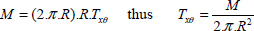
Where (2.π.R) corresponds to the circle’s perimeter, and the second R to the lever arm in order to calculate the moment.

Figure 15.7. Composite tube under torsion. For a color version of this figure, see www.iste.co.uk/bouvet/aeronautical2.zip
The best stacking sequence to support this shear resultant force is therefore a stacking sequence at ±45°, with 50% of plies at 45° and 50% at −45°. We can also place 10% of plies at 0° and at 90° to support a potential unpredicted load.
To complete the sizing of the tube, we should also verify that there is no local buckling (the shear is a tension at +45° and a compression at −45° that can cause buckling). The calculation is slightly more complicated, and you can find charts in the literature [GER 57], or use finite element calculation methods.
- – Bending: F = F.y in A
The case of bending is more complicated. We can show that the internal forces of the upper part of the beam on the lower part (by fictionally cutting the beam) decompose into a bending moment Mz and a shear force Ty:

In other words, the forces are maximum at the clamp (in x = 0), and if the beam should break, it would be at the clamp.
The bending moment will induce a tensile/compressive resultant force Nx linear in y (the resulting moment of which must be equal to Mz; see Figure 15.9(a)):

This resultant force Nx will be highest at the clamp (in x = 0) and at the top and bottom (in y = ±R). You could demonstrate this formula by remembering your knowledge of mechanics of material [AGA 08] and the famous:

Where Iz is the quadratic bending moment, which in this case is worth π.R3.e and by multiplying by thickness e to return to the resultant force.
As for the shear force Ty, it will cause a shear resultant force. This shear force is often left out of calculations because its effect is negligible in the case of a solid beam, which will not be the case here. To support loading along y-direction, the ideal solution would be to induce a shear stress τxy (we are located on a face of normal vector x), or a shear resultant force Txy (which is essentially the same thing). This does not pose a problem for the tube skin located around y = 0, as this shear is located in the plate plane, but it is impossible for the tube skin located around z = 0, as this shear then becomes an out-of-plane shear stress (Figure 15.8).
As the plate is thin, its ability to resist out-of-plane shear is low, compared to its ability to resist in-plane shear. We will therefore see the appearance of a shear resultant force Txθ, which will be maximum near y = 0 (in z = ±R) and null near z = 0 (in y = ±R); in sum, the plate can only support loading in its plane (Figure 15.8(b)). To calculate the resultant force, we can use the Bredt formula [AGA 08] which gives us the shear force resultant at a point A depending on its value in B:


Figure 15.8. Shear induced by shear force: if rigidity xy were the same everywhere a), and in reality b). For a color version of this figure, see www.iste.co.uk/bouvet/aeronautical2.zip
We can then say using symmetry, the shear force resultant must be null at y = ±R. We can then demonstrate that this shear force resultant is sinusoidal in θ (Figure 15.9(b)):


Figure 15.9. Composite tube under bending: stress resultant due to the bending moment a) and shear force b). For a color version of this figure, see www.iste.co.uk/bouvet/aeronautical2.zip
We can then determine the ply ratio in each direction (α, β, γ):

Remember to consider the maximum for Nx and Txθ throughout the structure. Once we know L and R, we can use these to determine the stacking sequence.
The drawback of this approach is that it only considers the maximum of the resultant forces. In reality, if we wished to optimize the weight of the tube, we would have to consider the resultant forces at each point and determine the stacking sequence in each point, which would obviously vary from one point to another. In the present case, the thickness of the laminate would be maximum at the level of the clamp and would be much lower at the end of the tube.
To complete the sizing of this tube, we would also have to verify that there is no local buckling (due to both the shear from the shear force and the compression from the bending moment). The calculation is even more complicated than previously, but you can refer to charts in the literature [GER 57] or perform a calculation using the finite element method.
- – Bending and torsion: F = F.y in A and M = M.x in A
This case is only the sum of the two previous cases:

The approach is therefore exactly the same, and if we consider the stacking sequence to be homogeneous throughout the structure, we obtain:

Even though, in reality, we would have to imagine a scalable stacking and remember to take buckling into account.
15.6. Laminate calculation without calculation
Consider the following four plates:
| Plate 1 | Plate 2 | Plate 3 | Plate 4 | |
|---|---|---|---|---|
| Ply 1 | 0° | 0° | 45° | 0° |
| Ply 2 | 90° | 90° | −45° | 0° |
| Ply 3 | Honeycomb | 90° | −45° | 0° |
| Ply 4 | 90° | 0° | 45° | 0° |
| Ply 5 | 0° | – | – | – |
Without using calculations, determine:
- – The plate with the highest bending stiffness:
It is obviously the sandwich plate (i.e. with two skins and honeycomb in the center), and therefore plate no. 1, which presents maximum bending stiffness. We restate that the bending stiffness varies with the cube of the thickness. This variation following the cube of the thickness appears both in the formula for the bending stiffness of a composite laminate plate:

and also in the famous formula for the bending stiffness of a rectangular solid beam:

Where b is the width of the beam and h the height.
- – The plate with the highest tensile stiffness along x-direction:
The plate presenting the most plies at 0°; therefore, plate no. 4 will be the one that has the highest tensile stiffness along x-direction.
- – The plate with the highest shear stiffness in the plane (x, y):
The plate presenting the most plies at ±45°; therefore, plate no. 3 will have the highest shear stiffness in (x, y). We restate that a shear stress is the sum of a tensile stress at +45° and a compressive stress at −45°, and that plies should be placed at +45° and at −45° to support this type of stress.
- – The ratio between the tensile stiffnesses along x- and y-directions:
For plate no. 1, this ratio will be equal to 1; in other words, the tensile stiffness is the same along x- and y-directions. When performing a rotation of 90°, the roles of the plies at 0° and 90° are simply being inverted. As for the tensile stiffness of the honeycomb along x- or y-directions, it is very low, and its effect on the overall tensile stiffness can be neglected (in practice, it is so low that it isn’t even provided by the supplier and is in the range of the kPa!). However, we will recall that the use of honeycomb is intended to separate the two skins and thus increase the bending stiffness. The only interesting honeycomb characteristics are its tensile/compressive characteristics along z-direction and its out-of-plane shear characteristics in the plane (x, z) and (y, z) (see the following exercise).
For plates 2 and 3, this ratio will also be equal to 1. For plate 2, the reasoning is the same as for the previous one, and for plate 3, performing a rotation of 90° simply inverts plies at +45° and at –45°.
For plate 4, this ratio will be equal to El/Et. Along x-direction, the tensile stiffness is equal to El, and along y-direction, the tensile stiffness will be equal to Et.
- – The plate with the highest fracture limit along x-direction:
The plate with the most plies at 0°; therefore, plate no. 4 will be the one that has the highest fracture limit along x-direction.
- – The plate with the highest buckling resistance along x-direction:
The plate with the highest bending stiffness; therefore, plate no. 1 will be the one that presents the highest resistance to buckling. We restate that the resistance to buckling along x-direction of a plate is both linked to bending stiffness D11 (which is along y-direction, and is thus linked to stress along x-direction, σx), but also to the other bending stiffnesses D22 (which is along x-direction, and is therefore linked to stress along y-direction, σy), D22, D12, D16, D26 and D66, and the link between the bending stiffnesses and buckling resistance of a plate is not straightforward (see Chapter 12).
15.7. Sandwich beam under bending

Figure 15.10. Sandwich beam under bending. For a color version of this figure, see www.iste.co.uk/bouvet/aeronautical2.zip
Question 1
The honeycomb is a very light material (typically a couple of tenths of kg/m3, in comparison to 1,000 kg/m3 for water or 1,700 kg/m3 for a typical carbon/epoxy laminate), which serves as the core in sandwich structures (one honeycomb plus two upper and lower skins). The honeycomb denomination comes from its evident resemblance to the honeycomb cells found in a beehive:

The three directions are generally called L for longitudinal (the stretching direction), W for the width and T for thickness.
There are two main categories of honeycomb made from sheets of aluminum or from Nomex® with a thickness of approximately 0.1 mm. Nomex® was originally the brand name for a type of aramid fabric sold by Du Pont de Nemours made out of aramid paper impregnated in a phenolic resin.
The advantage of inserting a layer of honeycomb between two skins is obviously to increase the bending stiffness (which varies depending on the cube of the thickness) for a reduced increase in mass (see question 6). The main interesting characteristics of honeycomb are its stiffness and resistance to tension/compression in the out-of-plane direction z and out-of-plane shear in the planes (x, z) and (y, z). Its other characteristics, Ex, Ey, σxr, σyr, Gxy, and τxyr, are very low and are not even provided by the supplier because they can be neglected when sizing.
Question 2
To determine the internal forces (force in the wider sense of the term, i.e. force in Newton, but also moment) from the right part of the beam to the left part, it is just a matter of isolating the right part of the beam and stating that the sum of the forces applying to this part is null.

Figure 15.12. Sandwich beam under bending. For a color version of this figure, see www.iste.co.uk/bouvet/aeronautical2.zip
You will easily find that the internal forces from the right part of the beam to the left part of the beam (since of course the force from left to right is equal to the opposite from right to left), thus the bending moment and the shear force:


Figure 15.13. Internal forces in a clamped beam under bending. For a color version of this figure, see www.iste.co.uk/bouvet/aeronautical2.zip
We note that the bending moment is maximum at the clamp, and that if there were to be a fracture, this is where the damage would initiate.
Question 3
The shear force will be supported by the intermediary of the shear stress τxz (cross-section of normal vector x and stresses along z-direction) and the bending moment by tensile/compressive stress σx (and we should verify that the sum of all these stresses is indeed worth zero in stress but not in moment; see Figure 15.14). In the case of a homogeneous solid cross-section, we can show that shear stress τxz is parabolic [AGA 08] (look closely at the following diagram; the blue dotted line indicates the distribution of stress τxz, but not their direction, which is in fact along z-direction!). It must, in particular, be null at the bottom and top due to the boundary conditions (null external forces above and below the beam), and the equilibrium equation written in the beam allows us to find the parabolic form from the linear form of σx. As for stress σx, we can show that it is linear in z. You will also note that τxz is constant throughout the length of the beam (along x-direction), whereas σx is also linear in x (and maximum at the clamp). If you do the math, you will find the classic result in the case of a homogeneous cross-section:

Where Iy is the quadratic bending moment:


Figure 15.14. Stresses in a clamped solid cross-section beam under bending. For a color version of this figure, see www.iste.co.uk/bouvet/aeronautical2.zip
Note, however, that these results are not valid in our case where the cross-section is not homogeneous. In reality, the stresses will have this form:

Figure 15.15. Stresses in a clamped sandwich cross-section beam under bending. For a color version of this figure, see www.iste.co.uk/bouvet/aeronautical2.zip
The shear stress τxz is once again null at the bottom and the top, but is practically constant throughout the honeycomb (again, look closely at the diagram; the blue dotted line indicates the distribution of stress τxz, but not its direction, which is, in fact along z-direction!). This is due to the fact that the tensile stiffness of the skins is much higher than that of the honeycomb (the Young’s modulus for the honeycomb along x-direction is practically 0). And we can demonstrate that the variation along z-direction of τxz (or ∂τxz/∂z) is equal (in absolute value) to the variation along x-direction of σx (or ∂σx/∂x). This comes from the equilibrium equation written for a planar stress in plane (x, z):

For more details surrounding these calculations, see [BAM 08, BER 99]. We can therefore initially suppose that the shear stress is null in the skins and constant in the honeycomb; thus:

Similarly, the tensile stiffness along x-direction is so low in the honeycomb that the generated stress σx will be low in comparison with the one in the skins. And since on top of that the thickness of the skins is low compared with the honeycomb, we can initially suppose that σx is constant in the skins. It is then just a matter of stating that the moment caused by these stresses is equal to the bending moment:

Thus:

And σx will be negative in the upper part of the beam and positive in the lower part of the beam.
We note, nonetheless, that this result is only true for the average stress (or if the skins are homogeneous along the thickness). To generalize this result to typical laminate layers, we would have to reason directly in the resultant forces and then state that the moment caused by these two resultant forces Nx is equal to the bending moment:

In conclusion, the cross-section of the beam that is the most loaded will be at the clamp, and we then get:

Where τxz is the shear stress in the honeycomb and Nx is the resultant force in the skins.
Question 4
To determine the deflection at the end of the beam, we should integrate the beam constitutive equation:

Using boundary conditions that w and its derivative according to x are null at the clamp. We will then find the classic formula for the deflection δM due to the bending moment:

However, this result is only strictly true for a beam with a homogeneous solid cross-section. In practice, we can show that it is also true for beams with non-solid and non-homogeneous cross-sections, on the condition that the correct bending stiffness E.Iy be used. In our case, it is just a matter of asking where the bending stiffness is coming from (the honeycomb is only included to separate the skins and support the shear force). Modulus E will therefore be the average modulus of the laminate along x-direction, and Iy will be the quadratic bending moment of the skins. To be exact, we would have had to calculate the bending stiffness of each of the plies following their orientations, but since the thickness of the honeycomb is far greater than the skins, using an average modulus does not affect the results much. I leave you to demonstrate that with the proposed laminate, you will find for the skins Ex = 51.4 GPa and the following quadratic bending moment:

Thus a deflection of δM = 259 mm.
We can note that the constitutive equation of a beam under bending is equivalent to that between a resultant moment Mx and the curvature k0x:

It should nonetheless be noted that Mx is a resultant moment in N.mm/mm and D11 is a plate bending stiffness in N.mm (whereas E.Iy is in N.mm2). Also note that the notation Mx means that this resultant moment is due to stresses along x-direction, σx, but that it is directed along y-direction. If we multiply this relation by the plate width b, we can then identify bending stiffness b.D11 of the plate of length b with bending stiffness E.Iy of the beam. Supposing that the modulus is constant throughout the thickness of the plate, we then obtain:

And you can show that in the case of a homogeneous isotropic material, we obtain:

The two formulae therefore differ simply from coefficient β (which, in a classic case where ν = 0.3, is worth 1.1). This difference comes from the hypothesis used in both the calculations. In the case of a beam, the thickness along y-direction is assumed to be small; we can therefore suppose that the stress is planar (σy = 0). In the case of a plate, the thickness along y-direction is high, and we will suppose that the strain is planar (εy = 0). In practice, we have b = h, and we are therefore closer to the beam hypothesis than the plate hypothesis.

Question 5
In the case of a homogeneous solid cross-section beam, we can show that the deflection due to shear force is negligible compared with that of the bending moment and is therefore often forgotten. In the case where the cross-section is more complex (for example, in the case of a beam with thin walls), this is not the case.
If we suppose that the shear stress τxz is homogeneous throughout the cross-section S of the beam, as is the case with honeycomb, we then have:

We can then determine the shear strain γxz, also assumed homogeneous in the whole cross-section of the beam, by:

and by definition of strain:

Therefore, we can show that the derivative of the displacement along x-direction, w(x), is equal to the shear strain [CHE 08]:

Thus the constitutive equation of a beam subject to a shear force:

As here the shear force is constant, we find the deflection resulting from shear force δT:

Where Gxz is the shear modulus of the honeycomb (here GLT), as we initially suppose that only the honeycomb supports the shear force. We observe that the deflection due to shear force remains lower than the one resulting from bending moment (but this is not always the case depending on the geometry of the problem and particularly if the thickness of the skins becomes small).
Question 6
The total deflection is therefore worth:

If we now suppose that there is no honeycomb, we can neglect the deflection resulting from shear force (it is then the case of a solid cross-section) and we have:

Where the Iy is that of a plate with a thickness of 2.e (equal to two times the thickness of the sandwich skins joined together), and E is the equivalent modulus of the laminate formed of the two previous skins Ex = 51.4 GPa. We then get a deflection:

Which is approximately 2 km!!! Of course this result makes no sense. In practice, we can show that a plate that is 2 mm thick, 100 mm wide and 2 m in length is of course unable to support a load of 2.5 kN, and that it will break far before reaching that load. To size it, we must study the most loaded cross-section (located at the clamp). This cross-section is subject to a bending resultant moment:

We must then determine the bending stiffness matrix composed of the two joined skins, i.e. [0, 45, 90, −45]2S:

We can then determine the curvatures:

Then the strains from:

as the membrane strains ε0 are null. We find a strain at the surface of the plate:

This strain is huge! If you are not convinced, you can determine the stress along the l-direction, σl, of the ply at 0° at the surface of the plate, and you will find 166,000 MPa! In sum, this beam is indeed unable to support a load of 2.5 kN without the honeycomb.
Question 7
To determine whether there is fracture of the sandwich beam, we begin by calculating if there is fracture within the skins. These skins are subject to a resultant force of ±500 N/mm, thus under tension (and with a Yamada–Sun criterion):
- – For plies at 0°: RF = 1.13
- – For plies at 90°: RF = 3.61
- – For plies at +45°: RF = 1.27
- – For plies at −45°: RF = 1.27
And in compression:
- – For plies at 0°: RF = 1.05
- – For plies at 90°: RF = 3.87
- – For plies at +45°: RF = 1.25
- – For plies at −45°: RF = 1.25
Therefore, the skins withstand, but barely (the data of the exercise were designed for this result).
We must also verify that the honeycomb does not break under shearing by verifying that the shear stress remains lower than its shear stress limit:

Which is verified here.
We should also verify that there is no delamination between the skin and the honeycomb. We must therefore initially verify that the shear stress in the honeycomb remains lower than the shear stress limit of the glue. The real problem is more complicated and goes beyond the scope of the present lesson. Readers interested in learning more about this can refer to [BER 99].
Finally, if the lower skin is subject to compression, we would have to verify that it does not buckle. The calculation is complex because the skin is glued to the honeycomb, and the compressive resultant force is not constant (linear variation along x-direction). This buckling would also tend to create a tensile stress along z-direction at the location of the bond between the skin and the honeycomb that could cause the fracture of the glue. Once again, readers interested in learning more can refer to [BER 99, GAY 97].
15.8. Laminate plate under compression
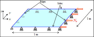
Figure 15.17. Simply supported panel under compression. For a color version of this figure, see www.iste.co.uk/bouvet/aeronautical2.zip
Question 1
The only resultant force being the compression along x-direction, we should take 100% of fibers at 0°. However, if we respect the 10% minimum fiber ratio in each direction rule, we will take 10% of plies at 90°, 10% at +45°, 10% at −45° and 70% at 0°. We must therefore determine the total thickness of the laminate to resist the compressive resultant force. Supposing that we know the thickness h of the laminate, we can determine the thickness of the plies in each direction:

We then determine the membrane stiffness of the laminate, which is linear in h:

Thus the strains, which in this case are homogeneous in the thickness of the laminate:

Thus:
- – For plies at 0°:

- – For plies at 90°:

- – For plies at +45°:

- – For plies at −45°:

Then, we apply a fracture criterion to each ply, for example a Yamada–Sun criterion:
- – For plies at 0°: 0.10/h ≤ 1
- – For plies at 90°: 0.08/h ≤ 1
- – For plies at +45°: 0.08/h ≤ 1
- – For plies at −45°: 0.03/h ≤ 1
We then use the maximum value of h in all the four directions, i.e.:

This value is largely less than the thickness of a single ply! In other words, compression will not be the one to determine the size, but rather buckling (in sum, the calculations we just made serve no purpose).
In order to respect the 10% rule, we need at least two plies at ±45° (to respect mirror symmetry), at least one ply at 90° (if it is at the center), and at least two plies at 0°, so for example a stacking sequence: [45, −45, 0, 900.5]S. This stacking sequence withstands the compressive loading without a problem:
- – For plies at 0°: RF = 9.96
- – For plies at 90°: RF = 25.4
- – For plies at 45°: RF = 11.2
- – For plies at −45°: RF = 11.2
However, we will see in the next question that it is far from supporting the buckling.
Question 2
With the stacking sequence [45, −45, 0, 900.5]S, we obtain:

Thus:

and:

This value is well below the force of −100 N/mm and the plate will buckle. This result is classic; we observe that a panel under compression is generally more sensitive to buckling than compression, and it is its buckling resistance that governs the stacking sequence and in particular its thickness.
Question 3
We can make an initial estimation of the necessary thickness to withstand buckling along x-direction noting that the buckling resistance increases with the cube of the thickness, thus the necessary thickness:

Upon the 1st approximation, we would thus have to multiply the thickness by 4.36 to resist buckling along x-direction, resulting in a thickness of 7.6 mm, and thus the 8 mm proposed in the data of the exercise. Of course this approximation is only valid while using the same stacking sequence, i.e. one using this type [45n, −45n, 0n, 900.5n]S. This type of stacking sequence should of course be avoided as it presents too many consecutive plies in the same direction, which has the effect of increasing interlaminar stresses.
The real problem is complicated because not only do we not know the thickness of the required laminate, but we do not know the ply ratio in each direction either. Unlike the case of a sizing with a given resultant force, where we can initially suppose that the ratio of fibers in each direction is proportional to the resultant force in that direction, here even those fiber ratios are unknown. The idea that fibers need to be placed at 0° to support the buckling from a compressive stress at 0° is false! This may seem odd, but it comes from the fact that a compressive buckling causes a 2D blister, and will therefore involve the bending stiffness of the laminate in all the directions. Add to that the fact that placing plies at ±45° disturbs the blister and thus tends to increase the buckling resistance; we reach the conclusion that there is nothing obvious! In practice, we often show that a ply at 90° is as effective as a ply at ±45°.
To simplify the problem, we will begin setting the total thickness of the laminate to 8 mm and review a number of stacking sequences. Using the method given by the ESDU 80023, we find the following critical buckling resultant forces:
Table 15.2. Calculation of buckling resistance, bending stiffnesses and RF for eight stacking sequences (the two pure UD stacking sequences are entirely textbook cases only included for the purpose of the study, but are not real-world stacking sequences!)
| Nxcr (N/mm) |
D11 (N.mm) |
D22 (N.mm) |
RF (0°) | RF (90°) | RF (±45°) | |
|---|---|---|---|---|---|---|
| [032] (textbook case) | 68 | 5.7 106 | 3.0 105 | 112 | – | – |
| [9032] (textbook case) | 35 | 3.0 105 | 5.7 106 | – | +∞ | – |
| [0, 90]8S | 68 | 4.0 106 | 2.0 106 | 59 | 5,364 | – |
| [0, 45, 90, −45]4S | 84 | 3.9 106 | 1.3 106 | 42 | 155 | 50 |
| [45, −45, 0, 90]4S | 113 | 2.1 106 | 1.6 106 | 42 | 155 | 50 |
| [45, −45]8S | 119 | 1.7 106 | 1.7 106 | – | – | 12 |
You will note that for the stacking sequence composed only of plies at 90°, the RF is infinite, because in that case, only σt is non-zero, and the Yamada–Sun criterion does not account for matrix cracking. In sum, the Yamada–Sun criterion only makes sense for a real stacking sequence and not for pure UD (the pure UD stacking sequences are textbook cases that are only present for the comparison but are not real-world stacking sequences!).
Finally, we observe that there must be plies at ±45° to support buckling along x-direction.
Question 4
The plies at 0° are better than plies at 90° because the blister caused by buckling may have two directions; the loading applied is along x-direction and will cause more bending resultant moment Mx than My. It should be kept in mind that even if applying a compressive resultant force will not cause bending resultant moment, once the plate is buckled, there will be many bending moments created (due to the deflection generated by buckling). Note, however, that this is not true in general cases! We can indeed show that in cases typically used in aviation (here the size of the plate is very large and square, whereas in aviation, they are generally smaller and rectangular, with the long side along the direction of the maximum compressive loading), adding a ply at 90° is better than adding a ply at 0°.
As for plies at ±45°, they tend to disturb the blister caused by buckling and therefore tend to increase the buckling resistance (see shape of the buckling blister in question 7). This result is always true and widely used in aviation!
Question 5
To make this panel lighter, we start by increasing its bending stiffness (the terms Dij of the bending stiffness matrix). For this, we can either increase the stiffness of the material, but we must then design a stiffer material (which can be difficult!), or distance the material from the midplane. The bending stiffness varies with the cube of the thickness, and therefore this second solution is much more efficient. We can therefore either modify the shape of the panel, by, for example, adding stiffeners, or make a sandwich panel by adding honeycomb. For example, if we add 10-mm-thick honeycomb to the 6th stacking sequence from the previous table, we get a stacking sequence of:

We then find:

By taking 1,700 kg/m3 for the volumic mass of the composite and 64 kg/m3 for that of the honeycomb, the panel goes from 13.6 to 14.2 kg, whereas its buckling resistance has practically been multiplied by 10! We must nonetheless keep in mind that the sandwich panels present a few drawbacks:
- – it is harder to introduce localized loading, and additional inserts are often required [GAY 97];
- – they absorb humidity, and the honeycomb cells tend to fill up with water (which will then freeze at −50 °C when the aircraft is operating);
- – they are more complicated to machine, and it is hard to make panels with complex shapes.
Question 6
We now focus on a stiffened panel with T-shaped stiffeners:

Figure 15.18. Stiffened panel under buckling. For a color version of this figure, see www.iste.co.uk/bouvet/aeronautical2.zip
In practice, there exist two main shapes of stiffeners: T shape and omega shape:

The T-shaped stiffeners are easy enough to manufacture because it is simply a matter of building them in the shape of a U, then joining them together to a flat plate. One final ply of composite is then generally added in order to avoid stiffener delamination. Here are two industrial fuselage panel realizations made up of San Diego Composites® and Muratec®; you will also be able to find more online.

Figure 15.20. Fuselage with omega-shaped stiffeners (San Diego Composites®) and a low-cost composite fuselage with T-shaped stiffeners (Muratec®)
Question 7
To simplify the problem, we will limit ourselves to T-shaped stiffeners of 40 mm height, sitting at 200 mm from one another, and we will consider the same stacking sequence for the skin and the stiffeners:

By keeping stacking sequences of type ±45°, we find that the following stacking sequence allows us to maintain a critical buckling load higher (in absolute value) than −100 N/mm:

Therefore, 22 plies are required instead of the 32 plies for the flat panel, meaning a stiffened panel of 10.8 kg rather than 13.6 kg for the flat panel. Of course this optimization is far from optimal, and we can test stiffeners with different geometries, stacking sequences, variable thicknesses in the panel and the stiffeners…
Furthermore, it becomes difficult to perform analytical calculations (even if methods exist, for example in [ESD 95]), and we often resort to calculations using the finite element method. For the studied case, the 1st buckling modes for flat and stiffened panels are as follows:

Figure 15.22. First buckling modes of a flat panel [45, −45]8S and a panel with T-shaped stiffeners [(45, −45)5, 45]S (the perspective of the stiffened panel can be deceiving; the panel is seen from below and the blister is facing away from the stiffeners). For a color version of this figure, see www.iste.co.uk/bouvet/aeronautical2.zip
We therefore typically find the 1st buckling mode in the form of a single buckling blister (which is not necessarily the case depending on the shape of the panel). The finite element calculation gave us Nxcr = 105 N/mm for the flat panel [45, −45]8S, in comparison to Nxcr = 117 N/mm that we found analytically. The main difference comes from the chart of the ESDU 8023 which assumes that the components D16 and D26 of the bending matrix are null, which here is not the case. The finite element/analytical correlation nonetheless remains correct, but is even better for stacking sequences with null D16 and D26 components (or low). You will also note that in the previous figure, the maximum displacement is equal to 1. We can show that if the applied loading is equal to the critical buckling force, the solution to the problem is not unique, but rather determined to within a multiplicative coefficient (the buckling mode is an eigenvector of the stiffness matrix). In other words, if you take the solution from the previous figure and multiply the displacement field by a given coefficient, the new displacement field will always yield the solution to the problem. It is therefore common practice to arbitrarily select a maximum displacement of 1 (1 mm in this case), then apply a multiplicative coefficient to better identify the structure deformed shape (in this case, we used a coefficient 100). In reality, if we wished to study the development of the buckling mode in more detail, we would have to use a nonlinear calculation.
We can also optimize the panel by adding transverse stiffeners along y-direction. In the case of aviation structures, we generally make sure we achieve the first buckling mode that buckles the skin-stiffened panel, i.e. the plate located between two consecutive stiffeners along x- and y-directions. In the case of a passenger plane type A320, the distance between the longitudinal stiffeners (these stiffeners are directed along the axis of the fuselage and are also called the stringers) is approximately 200 mm and approximately 600 mm between circumferential stiffeners (these stiffeners along the circumferential direction are therefore more or less circular and are called the frames). Using these distances approximately, we therefore choose to add a transverse T-shaped stiffener in y-direction at the middle of the panel (this obviously avoids global buckling as was the case for the previous panel). In practice, the cross-section for these transverse stiffeners is higher than that of the longitudinal stiffeners; here, we select a height of 60 mm (40 mm for the longitudinal stiffeners). Evidently, the optimization problem then becomes far more complicated because the number of variable parameters becomes much higher: panel stacking sequence, stacking sequence and height of the longitudinal stiffeners, stacking sequence and height of the transverse stiffeners (and in reality, the shape of the stiffeners still needs optimizing). We choose to stay with a 22 ply stacking sequence [(45, −45)5, 45]S for the stiffeners and opt for a stacking sequence for the skins that will allow for buckling of the skin-stiffened panel (a 500 mm-long and 200 mm-wide plate). Maintaining a stacking sequence using plies at ±45° leads to a stacking sequence of 12 plies [45, −45]3S (you can also verify that the RF remain largely higher than 1). The optimization of the skin-stiffened panel can also be performed using the compression chart: you would find here a buckling for this panel that is 500 mm long and 200 mm wide for a resultant force of 158 N/mm. In this case, you can even demonstrate that 11 plies would have been enough, but a calculation using finite element method shows that the skin-stiffened panel would have buckled too early in the case of the full-sized panel (the stiffeners are obviously not infinitely stiff and therefore do not exactly impose null out-of-plane displacements).
Using a finite element calculation of the full-sized panel, we obtain buckling for Nxcr = 113 N/mm and a weight of the panel of 7.2 kg:

Figure 15.23. Buckling of a stiffened panel with longitudinal and transverse stiffeners. For a color version of this figure, see www.iste.co.uk/bouvet/aeronautical2.zip
This design method using longitudinal and transverse stiffeners, making sure to buckle the skin-stiffened panel first, is very interesting for optimizing the mass of a panel, even if it does complicate the design process somewhat. It is obviously no coincidence that practically all planes are designed this way!
15.9. Tube under torsion/internal pressure

Figure 15.24. Composite tube under torsion/internal pressure. For a color version of this figure, see www.iste.co.uk/bouvet/aeronautical2.zip
Question 1
The torsion moment will cause a shear resultant force Tzθ. If we cut the laminate along a face of normal vector z, the resultant force is then directed along θ-direction. To determine the shear resultant force, simply sum the moment caused by these arrows (Figure 15.25):

Where (2.π.R) corresponds to the circle’s perimeter, and the second R to the lever arm for the calculation of the moment.
As for the internal pressure, it will cause a tensile resultant force Nθ. This resultant force corresponds to a resultant force along θ-direction for a cut by a face with normal vector θ. To determine this resultant force, simply state that the half-cylinder is balanced under the effect of Nθ and pressure P. To integrate pressure P on a half-circle, it is important to account for the fact that the direction of P varies depending on the considered point; therefore, either integrate considering the projection of P along x-direction (which will highlight an angle θ that varies between –π/2 and π/2), or you can remember that the integral gives the pressure P multiplied by the projected surface area. You will also note that the calculation does not highlight the length along z-direction, in other words, it corresponds to a unit length (in N/mm). We then have:


Figure 15.25. Resultant force under torsion a) and internal pressure b). For a color version of this figure, see www.iste.co.uk/bouvet/aeronautical2.zip
Question 2
We can then determine the ply ratio in each direction (α, β, γ):

Omitting the 10% rule to simplify the problem. If we add that the sum of the ply ratios is obviously 100%, and considering a ratio of γ at +45° and at −45° (α + β + 2.γ = 1) :

We can then reuse the proposed procedure in exercise 8, or simply test some numbers of plies. Here, you will find that two plies along ±45°-direction and four plies at 90° are enough (with the Yamada–Sun criterion):
- – For 4 plies at 90°: RF = 1.06
- – For 2 plies at 45°: RF = 1.08
- – For 2 plies at −45°: RF = 1.21
Therefore, for example, the following stacking sequence:

This allows us to maintain a mirror symmetry and avoid too many consecutive plies in the same direction.
Question 3
The tube being made from filament winding, we can easily create stacking sequences with any given directions. Nonetheless, in order to avoid tension/shear coupling, we will use as many plies at +α as we do at –α (you can verify that in this case, A16 and A26 are null). The calculation procedure in plies at α is similar to classic plies at 0°, 90° or ±45°, outside of the shape of the stiffness matrices  which of course is more complicated (see Chapter 3). We can then vary angle α and determine the number of plies that result in RF higher than 1. Since there is no loading along z-direction, we will simply vary this angle between 45° and 90° (the solutions between 0° and 45° are also far less interesting). We denote as n the number of plies at α (and thus also at –α), and get:
Table 15.3. Calculation of a stacking sequence for a tube under torsion/internal pressure
| α | 45° | 50° | 55° | 60° | 65° | 70° | 75° | 80° | 85° | 90° |
| n | 14 | 12 | 9 | 7 | 6 | 5 | 6 | 8 | 12 | 14 |
| RF | 1.03 | 1.07 | 1.01 | 1.04 | 1.13 | 1.05 | 1.12 | 1.07 | 1.07 | 1.02 |
The best solution is therefore 5 plies at 70° and 5 plies at −70°. We then find a stacking sequence of the following type:

And the optimal stacking sequence is therefore worse than the traditional stacking sequence with plies at 0°, ±45° and 90° (10 plies against 8). In conclusion, the obligation to place as many plies at +α and –α is more restrictive than placing plies at 0°, ±45° and 90°. Note, however, that this conclusion is not always true! Furthermore, in reality, filament winding allows us to stack in any direction. Lastly, keep in mind that using filament winding makes it simpler to stack plies at ±α than at ±45° and 90°.
15.10. Optimization of a fabric with a strain fracture criterion

Figure 15.26. Ply of 8 harness satin fabric. For a color version of this figure, see www.iste.co.uk/bouvet/aeronautical2.zip
Part I: preamble
Question 1
Here, we are working with a balanced fabric, meaning that the fiber ratio is the same along l- and t-directions; thus, approximately 25% (of the total volume) is fibers in l-direction, 25% are in t-direction, and 50% fibers resin. In reality, even when a fabric is balanced, its characteristics are slightly different along l- and t-directions; we observe that the warp direction (the one that was under tension during weaving) is stiffer and more resistant than the weft direction (typically 10–20% more). This comes from the fact that the warp fibers oscillate less than the weft ones do, because the warp is stretched during weaving. In this exercise, we suppose that the characteristics are the same for both the directions l and t to simplify the calculations. Furthermore, the use of a strain criterion allows the calculations to be made even simpler.
The compliance matrix of the ply at 0° is simply (both in (x, y) and (l, t)):

Question 2
The stiffness matrix of the ply at 0° is (both in (x, y) and (l, t)):

Question 3
The compliance matrix of the ply at 45° is:

S16 and S26 (like Q16 and Q26) are null because there are as many fibers at +45° as there are at −45° and because the behavior is assumed the same along l-direction as it is along t-direction.
Question 4
The stiffness matrix of the ply at 45° is:

The term Q66 of a ply at 45° is of course much higher than that of the ply at 0°. We see that the one for the ply at 45° is linked to modulus E, whereas the one for the ply at 0° is linked to G. This comes from the fact that a ply of fabric at 45° has fibers at +45° and at −45°, allowing it to support the stresses caused by shearing (a tension at +45° and a compression at −45°).
Part II: quasi-isotropic stacking sequence
Question 5
To determine the Young’s modulus along x-direction of a laminate composed of two plies of fabric at 0° and at 45°, we then begin by determining the stiffness matrix A of the laminate:

We invert the matrix to determine the compliance matrix of the laminate:

We can then relate this matrix to the compliance matrix of a homogeneous material (without forgetting thickness h) (see exercise 3):

Thus:

Question 6
The material is quasi-isotropic because there are the same amount of fibers at 0°, at 90°, at +45° and at −45° (and the behavior of the fabric along the l-direction is the same as along the t-direction); thus, the modulus will be the same in all the directions (see Chapter 6). We then have:

Question 7
To determine the limit shear stress τxy0, simply take a stress τxy0, then determine the RF in each ply. The limit stress will be, by definition of the RF (the coefficient by which we must multiply the load to obtain fracture), the minimum of the RF multiplied by the selected stress τxy0.
We restate that τxy0 is the average shear stress, i.e.:

Where e is the thickness of the laminate (here 2 mm). The drawback of this average stress is that no ply actually experiences it (therefore in particular, using this stress for a fracture criterion makes no sense).
Let us take an average stress of 100 MPa:

We can then determine the membrane strains:

Then the strains in each ply:

All that is left to do is determine the RF using the strain criterion and taking the minimum RF between directions l and t:

Thus:
- – For plies at 0°: RF = +∞
- – For plies at 45°: RF = 1.89
In the plies at 0°, the strains along l- and t-directions were null, and we find an infinite RF. This is due to the criterion we are using which does not account for shear strain, but rather only the strains in the fiber direction. In reality, this criterion only makes sense if we have at least one ply at 0° and one ply at 45°. In the present case, the infinite RF means that only plies at 45° support the loading (which is only true upon initial approximation).
The stress limit will therefore be the 100 MPa we selected, multiplied by the minimum RF; thus:

Question 8
To determine the RF for a given stress, we use the same procedure:

Thus, the strains in each ply:

Thus:
- – For plies at 0°: RF = 0.33
- – For plies at 45°: RF = 0.38
The proposed stacking method does not withstand the proposed load.
Question 9
To determine a stacking sequence that will withstand this loading, we simply note that the RF are linear depending on the thickness. Note, however, that this is only true under membrane loading, but not under bending loading. In other words, when we multiply the thickness of a laminate by two, we are dividing the RF by two as well (if we consider that the stacking sequence remains the same, and with plies twice as thick). Therefore, here it is just a matter of taking three times the stacking sequence plus a little extra something, an added ply at 0° for example, which would give us:

Furthermore, we avoid placing plies at 0° on the surface, because these are the ones that will support the most load (Nx = −1,500 N/mm). Redoing the calculations for this stacking sequence, we then get:
- – For plies at 0°: RF = 1.10
- – For plies at 45°: RF = 1.18
Part III: stacking sequence optimization
Question 10
We begin by supposing that the fiber ratio in each direction is proportional to the corresponding resultant force (note that it is impossible to place fibers at 0° without having any at 90° in this case):

If we add that the sum of the ratios is for obvious reasons 100% (α + γ = 1) , then:

We name h the thickness of the laminate, and get:

Thus the strains, which in this case are homogeneous throughout the thickness of the laminate:

Thus:
- – For plies at 0°:

- – For plies at +45°:

We then apply the strain criterion in each ply:
- – For plies at 0°: h ≥ 5.18 mm
- – For plies at +45°: h ≥ 6.76 mm
Of course we select the maximum value of h for all four directions, i.e.:

Thus:
- – For plies at 0°: e0° ≥ α.h = 4.8 mm
- – For plies at +45°: e45° ≥ γ .h = 2.0 mm
For example:

By redoing these calculations for this stacking sequence, we would find:
- – For plies at 0°: RF = 1.35
- – For plies at 45°: RF = 1.03
We find a solution that is heavier than the previous one (7 mm against 6.5 mm). This comes from the fact that the proposed method is adapted to a stacking sequence with plies at 0°, 90° and ±45°, but in this case, it is impossible to have fibers at 0° and none at 90°. In other words, when we place a ply at 0° to support the load along x-direction, the fibers at 90° no longer serve a purpose.
Part IV: stacking sequence optimization under bending
Question 11
Consider a stacking sequence formed of two plies at 0° and six plies at 45°. In the general case, we would choose the following type of stacking sequence:

This type of stacking sequence avoids having too many consecutive plies in the same direction and avoids having the plies at 0°, the ones supporting the load, at the surface.
In the present case, if we want to support a resultant moment Mx, we had best place the plies at 0° at the surface to support this moment, i.e.:

However, in practice, this stacking sequence is prohibited as it is forbidden to place the plies supporting the load (the ones at 0° in this case) at the surface, and we will always favor plies at ±45° on the surface to increase the buckling resistance. Furthermore, we cannot have six consecutive plies in the same direction to limit interlaminar stresses and thus delamination. Therefore, we will maintain the previous stacking sequence option:

To determine the fracture resultant moment Mxf, it is simply a matter of supposing any given resultant moment Mx, for example, Mx = 100 N, then calculating the RF in each ply. Note, however, that in the case of a bending loading, the RF vary linearly throughout the thickness; they are therefore maximum/minimum at the top or bottom of each ply (or of each group of consecutive plies in the same direction). The fracture resultant moment will then be, by definition of the RF (the coefficient by which we must multiply the load to obtain the fracture), the minimum of the RF multiplied by the selected resultant moment Mx.
We therefore begin by determining the stiffness matrix under bending:

We can then determine the curvatures:

And the strains from:

We then obtain a linear strain field along the thickness, null at the center and mainly composed of strains εx:

Figure 15.27. Strains of the laminate under bending Mx. For a color version of this figure, see www.iste.co.uk/bouvet/aeronautical2.zip
The minimum/maximum RF are achieved at the top of the upper ply at 0°, at the bottom of the lower ply at 0°, at the top of the upper surface ply at 45° and at the bottom of the lower surface ply at 45° (for plies at 45°, the strains in (l, t) must of course be determined beforehand):
- – At the top of the upper ply at 45°: RF = 18.6
- – At the top of the upper ply at 0°: RF = 6.93
- – At the bottom of the lower ply at 0°: RF = 8.53
- – At the bottom of the lower ply at 45°: RF = 22.8
Thus:

15.11. Open hole tensile test
Question 1
In the absence of a hole, it is just a matter of supposing a resultant force along x-direction, for example Nx = 100 N/mm, then calculating the RF within each ply. The fracture resultant force will then be, by definition of the RF (the coefficient by which we must multiply the loading to obtain the fracture), the minimum of the RF multiplied by the selected resultant force Nx.

We begin by determining the membrane stiffness matrix of the laminate:

We can then determine the membrane strains:

Then the strains in each ply:

All that is left to do is determine the RF using the strain criterion and using the minimum RF between directions l and t:

Thus:
- – For plies at 0°: RF = 20.4
- – For plies at 45°: RF = 60.0
Thus, the following fracture resultant force in the absence of a hole:

Question 2
To determine the equivalent moduli of the woven laminate, we begin by determining the stiffness matrix of the laminate, inverting it in order to determine the compliance matrix of the laminate, then relating the matrix to the compliance matrix of a homogeneous material (without forgetting thickness h) (see exercise 3):

Thus:

Question 3
The resultant force concentration ratio at the hole edge (i.e. the ratio between the maximum resultant force obtained at the hole edge and the far-field resultant force) is here:

Supposing that the fracture takes place where the resultant force is highest, i.e. at the hole edge (which in this case is not so simple, as we will see in the coming questions), the fracture resultant force Nxhole in the presence of a hole will thus be:

Of course, this result does not depend on the size of the hole, just like the resultant force concentration ratio at the hole edge. In reality, we can show that this is not the case, because the smaller the hole, the more the composite will get damaged at the hole edge (in proportion to the size of the hole), and the less this hole will be a problem.
Question 4
The previous calculation that allows us to determine the stress at the hole edge only works if the material is linear elastic, and if the plate remains a plate. And at the hole edge, the material gets damaged. Therefore, not only is the behavior of the material no longer linear elastic, but also the laminated plate theory we presented previously is no longer valid (in particular, the damage at the hole edge will cause small delaminations and the plies of the laminate are no longer perfectly bonded, and the model of homogeneous strains through the thickness for a membrane loading is no longer true). And since the size of the damaged area is, upon initial approximation, constant depending on the size of the hole (the size of the damaged area will be proportionally larger if the hole size is small), a small hole is therefore less dangerous than a large hole. The “point stress” theory allows us to account for this effect, supposing that the calculation of the stresses is true only from a certain distance from the hole:

Figure 15.29. Principle of the “point stress” theory. For a color version of this figure, see www.iste.co.uk/bouvet/aeronautical2.zip
We therefore begin by determining the resultant force concentration ratio at the hole edge for the three diameters:


Figure 15.30. Hole size effect of holed plate under tension and accounting for this using the “point stress” theory. For a color version of this figure, see www.iste.co.uk/bouvet/aeronautical2.zip
We use this to evaluate from which value of α we achieve this concentration ratio, and therefore the corresponding distance d0:

We therefore find values of d0 included between 1 and 2 mm, which are characteristic values of composite aircraft structures. Of course, if the point stress method were perfect, we would find the same value of d0 for all the radii of the holes, and if possible, for all the stacking sequences and thicknesses of the laminates. The reality is, as is often the case, more complicated than the small model you would like them to fit into. In industrial use, it is common to build charts of d0 according to the radius and stacking sequence in use.
15.12. Multi-bolt composite joint
Question 1
We will begin by evaluating the size of the current area (i.e. outside the joint area) of plate 1. The problem comes down to finding a stacking sequence that is resistant to resultant forces Nx = 1,500 N/mm and Ny = 1,000 N/mm. I will let you verify that stacking sequence [45, −45, 0, 90, 00.5]S (thus 9 plies and a total thickness of 2.25 mm) is suitable and gives using a Yamada–Sun criterion:
- – For plies at 0°: RF = 1.24
- – For plies at 90°: RF = 1.78
- – For plies at 45°: RF = 1.43
- – For plies at −45°: RF = 1.43

Now we size the current area of plate 2. The problem comes down to finding a stacking sequence that is resistant to resultant force Nx = 1,500 N/mm. I will let you verify that a stacking sequence [45, −45, 0, 90, 00.5]S (thus 9 plies and a total thickness of 2.25 mm) is still suitable and gives using a Yamada–Sun criterion:
- – For plies at 0°: RF = 1.00
- – For plies at 90°: RF = 3.22
- – For plies at 45°: RF = 1.13
- – For plies at −45°: RF = 1.13
And surprisingly, we obtain that the RF of the plies at 0° and ±45° decreases when the resultant force along y-direction is null! This is fairly common and explains in part why we always have 10% of plies in each direction, to not have to verify all the intermediary loads, linear combination of maximum loads.
We will now focus on the joint area. We begin by choosing the pitch distance, i.e. the distance between two consecutive holes. In practice, the pitch distance must be at least equal to approximately four times the diameter of the hole in all the directions; we choose to use a pitch distance of 4.D (a typical value, often used in aviation):

Where D is the diameter of the hole (and therefore the rivet) and W the distance between two consecutive rivets. We can then determine the equivalent stress, σxeq, defined by the stress leading to the same level of damage (or even the RF) as in the absence of the hole (see Chapter 11):

We must nonetheless note the thickness of the plate, because it can be different between the current area and the joint area (we often increase the thickness of the multi-bolt joint to withstand overloads due to the joint). Naming ej the thickness of the joint area, we can determine the net stress at the joint:

α is the hole ratio; therefore, for this case of tensile stress:

Kb is the bearing ratio (see Chapter 11):

and σb the bearing stress defined by:

Where Frivet is the bearing force transmitted by each rivet (this force depends on the number of rivets). To determine this bearing force, it is necessary to know the number of rivets. We begin by choosing two rivets (and we will increase the number of rivets if they are not enough!); we therefore have 50% of the force passing through the 1st rivet and 50% through the second, or:

We then obtain:

Along y-direction, the problem is simple; the force no longer passes in the rivets and only passes in plate 1. We then get:


Figure 15.32. Diagram of the multi-bolt composite joint with varying thickness. For a color version of this figure, see www.iste.co.uk/bouvet/aeronautical2.zip
Plate 1 is therefore subject in the joint area to:

Where ej is the thickness of the plate in the joint area, and it is therefore different to the thickness in the current area previously determined (it will likely be thicker). To determine the stacking sequence that is resistant to this load, it must also be noted that we will have to impose continuity between this stacking sequence and the current area (by performing ply drop-offs). It is therefore important to maintain the previous plies and add other to support this load. I will let you verify that the stacking sequence [45, −45, 02, 90, 02, 90, 01.5]S (therefore, 19 plies and a total thickness of 4.75 mm) is suitable for the two plates and gives us, for plate 1:
- – For plies at 0°: RF = 1.16
- – For plies at 90°: RF = 1.15
- – For plies at 45°: RF = 1.16
- – For plies at −45°: RF = 1.16
And for plate 2:
- – For plies at 0°: RF = 1.06
- – For plies at 90°: RF = 5.30
- – For plies at 45°: RF = 1.24
- – For plies at −45°: RF = 1.24
We must then show that this stacking method resists bearing. This bearing load corresponds to the maximum load passing in a rivet; therefore, here:

Knowing that this stress must remain below the bearing limit stress, thus approximately 600 MPa (or −600 MPa to be specific, since it is a case of compression) for the considered T300/914. This condition is therefore not entirely verified, but if we add a ply, at 0° for example, for a stacking sequence such as [45, 0, −45, 02, 90, 02, 90, 0]S (thus, 20 plies and a total thickness of 5 mm), the condition is respected:

And I will let you verify that the RF are still higher than 1.
To finish defining a multi-bolt joint, all that remains is to select the hole distance at the edge of the plate; for example, we can use a hole edge distance equal to 3.D (see previous figure).
Question 2
There is of course no point in taking the same stacking sequence in the joint as in the current area. We will therefore have to perform ply drop-offs to go from one stacking sequence to other, for example:

Figure 15.33. Ply drop-offs at the edge of the multi-bolt joint. For a color version of this figure, see www.iste.co.uk/bouvet/aeronautical2.zip
In this diagram, you will note that we have opted to perform these ply drop-offs in a quasi-symmetrical manner, but this is not necessarily always the case. The rules for ply drop-offs are outside the scope of this book, and curious readers can refer to [BER 99, GAY 97] for more details. You can nonetheless retain the two main rules:
- – You should distribute the ply drop-offs through the thickness and impose a slope of approximately 1/20, thus, 5 mm between two consecutive ply drop-offs for a ply thickness of 0.25 mm. In the present case, we would need a distance of approximately 55 mm to stop the 11 plies.
- – Each stopped ply must, if possible, be covered by a continuous ply (this rule is often difficult to respect, and it is in fact not the case here).
In reality, the real geometry of a ply drop-off is of course more complex than the corresponding diagram. For example, here are the differences we can observe between a real and a theoretical ply drop-off [ABD 15]:

Figure 15.34. Real and theoretical ply drop-offs [ABD 15]. For a color version of this figure, see www.iste.co.uk/bouvet/aeronautical2.zip
We had also better perform these ply drop-offs as far as possible from the force transmission plane to avoid bending moments in the joint. You will note that in the previous figure (Figure 15.33), the sum of the applied moments at the joint is non-zero due to the gap of the midplane of the two plates. We had therefore also better align the two laminate midplanes to avoid this parasitic moment:

Figure 15.35. Multi-bolt joint with alignment of the midplanes. For a color version of this figure, see www.iste.co.uk/bouvet/aeronautical2.zip
Even in reality, there is often a stiffener to support this bending moment. Since in aviation there are generally a lot of stiffeners, we practically always make sure that the joint coincides with a stiffener:

Figure 15.36. Multi-bolt joint with stiffener. For a color version of this figure, see www.iste.co.uk/bouvet/aeronautical2.zip