DATA SCIENCE is discussed and some important connections, and contrasts, are drawn between statistics and data science. A brief discussion of big data is provided, the Julia language is briefly introduced, and all Julia packages used in this monograph are listed together with their respective version numbers. The same is done for the, albeit smaller number of, R packages used herein. Providing such details about the packages used helps ensure that the analyses illustrated herein can be reproduced. The datasets used in this monograph are also listed, along with some descriptive characteristics and their respective sources. Finally, the contents of this monograph are outlined.
What is data science? It is an interesting question and one without a widely accepted answer. Herein, we take a broad view that data science encompasses all work related to data. While this includes data analysis, it also takes in a host of other topics such as data cleaning, data curation, data ethics, research data management, etc. This monograph discusses some of those aspects of data science that are commonly handled in Julia, and similar software; hence, its title.
The place of statistics within the pantheon of data science is a topic on which much has been written. While statistics is certainly a very important part of data science, statistics should not be taken as synonymous with data science. Much has been written about the relationship between data science and statistics. On the one extreme, some might view data science — and data analysis, in particular — as a retrogression of statistics; yet, on the other extreme, some may argue that data science is a manifestation of what statistics was always meant to be. In reality, it is probably an error to try to compare statistics and data science as if they were alternatives. Herein, we consider that statistics plays a crucial role in data analysis, or data analytics, which in turn is a crucial part of the data science mosaic.
Contrasting data analysis and mathematical statistics, Hayashi (1998) writes:
… mathematical statistics have been prone to be removed from reality. On the other hand, the method of data analysis has developed in the fields disregarded by mathematical statistics and has given useful results to solve complicated problems based on mathematico-statistical methods (which are not always based on statistical inference but rather are descriptive).
The views expressed by Hayashi (1998) are not altogether different from more recent observations that, insofar as analysis is concerned, data science tends to focus on prediction, while statistics has focused on modelling and inference. That is not to say that prediction is not a part of inference but rather that prediction is a part, and not the goal, of inference. We shall return to this theme, i.e., inference versus prediction, several times within this monograph.
Breiman (2001b) writes incisively about two cultures in statistical modelling, and this work is wonderfully summarized in the first few lines of its abstract:
There are two cultures in the use of statistical modeling to reach conclusions from data. One assumes that the data are generated by a given stochastic data model. The other uses algorithmic models and treats the data mechanism as unknown. The statistical community has been committed to the almost exclusive use of data models. This commitment has led to irrelevant theory, questionable conclusions, and has kept statisticians from working on a large range of interesting current problems.
The viewpoint articulated here leans towards a view of data analysis as, at least partly, arising out of one culture in statistical modelling.
In a very interesting contribution, Cleveland (2001) outlines a blueprint for a university department, with knock-on implications for curricula. Interestingly, he casts data science as an “altered field” — based on statistics being the base, i.e., unaltered, field. One fundamental alteration concerns the role of computing:
One outcome of the plan is that computer science joins mathematics as an area of competency for the field of data science. This enlarges the intellectual foundations. It implies partnerships with computer scientists just as there are now partnerships with mathematicians.
Writing now, as we are 17 years later, it is certainly true that computing has become far more important to the field of statistics and is central to data science. Cleveland (2001) also presents two contrasting views of data science:
A very limited view of data science is that it is practiced by statisticians. The wide view is that data science is practiced by statisticians and subject matter analysts alike, blurring exactly who is and who is not a statistician.
Certainly, the wider view is much closer to what has been observed in the intervening years. However, there are those who can claim to be data scientists but may consider themselves neither statisticians nor subject matter experts, e.g., computer scientists or librarians and other data curators. It is noteworthy that there is a growing body of work on how to introduce data science into curricula in statistics and other disciplines (see, e.g., Hardin et al., 2015).
One fascinating feature of data science is the extent to which work in the area has penetrated into the popular conscience, and media, in a way that statistics has not. For example, Press (2013) gives a brief history of data science, running from Tukey (1962) to Davenport and Patil (2012) — the title of the latter declares data scientist the “sexiest job of the 21st century”! At the start of this timeline is the prescient paper by Tukey (1962) who, amongst many other points, outlines how his view of his own work moved away from that of a statistician:
For a long time I have thought I was a statistician, interested in inferences from the particular to the general. … All in all, I have come to feel that my central interest is in data analysis, which I take to include, among other things: procedures for analyzing data, techniques for interpreting the results of such procedures, ways of planning the gathering of data to make its analysis easier, more precise or more accurate, and all the machinery and results of (mathematical) statistics which apply to analyzing data.
The wide range of views on data science, data analytics and statistics thus far reviewed should serve to convince the reader that there are differences of opinion about the relationship between these disciplines. While some might argue that data science, in some sense, is statistics, there seems to be a general consensus that the two are not synonymous. Despite the modern views expounded by Tukey (1962) and others, we think it is fair to say that much research work within the field of statistics remains mathematically focused. While it may seem bizarre to some readers, there are still statistics researchers who place more value in an ability to derive the mth moment of some obscure distribution than in an ability to actually analyze real data. This is not to denigrate mathematical statistics or to downplay the crucial role it plays within the field of statistics; rather, to emphasize that there are some who value ability in mathematical statistics far more than competence in data analysis. Of course, there are others who regard an ability to analyze data as a sine qua non for anyone who would refer to themselves as a statistician. While the proportion of people holding the latter view may be growing, the rate of growth seems insufficient to suggest that we will shortly arrive at a point where a statistician can automatically be assumed capable of analyzing data.
This latter point may help to explain why the terms data science, data scientist and data analyst are important. The former describes a field of study devoted to data, while the latter two describe people who are capable of working with data. While it is true that there are many statisticians who may consider themselves data analysts, it is also true that there are many data analysts who are not statisticians.
Along with rapidly increasing interest in data science has come the popularization of the term big data. Similar to the term data science, big data has no universally understood meaning. Puts et al. (2015) and others have described big data in terms of words that begin with the letter V: volume, variety, and velocity. Collectively, these can be thought of as the three Vs that define big data; however, other V words have been proposed as part of such a definition, e.g., veracity, and alternative definitions have also been proposed. Furthermore, the precise meaning of these V words is unclear. For instance, volume can be taken as referring to the overall quantity of data or the number of dimensions (i.e., variables) in the dataset. Variety can be taken to mean that data come from different sources or that the variables are of different types (such as interval, nominal, ordinal, binned, text, etc.). The precise meaning of velocity is perhaps less ambiguous in that it is usually taken to mean that data come in a stream. The word veracity, when included, is taken as indicative of the extent to which the data are reliable, trustworthy, or accurate. Interestingly, within such three (or more) Vs definitions, it is unclear how many Vs must be present for data to be considered big data.
The buzz attached to the term big data has perhaps led to some attempts to re-brand well-established data as somehow big. For instance, very large databases have existed for many years but, in some instances, there has been a push to refer to what might otherwise be called administrative data as big data. Interestingly, Puts et al. (2015) draw a clear distinction between big data and administrative data:
Having gained such experience editing large administrative data sets, we felt ready to process Big Data. However, we soon found out we were unprepared for the task.
Of course, the precise meaning of the term big data is less important than knowing how to tackle big data and other data types. Further to this point, we think it is a mistake to put big data on a pedestal and hail it as the challenging data. In reality there are many challenging datasets that do not fit within a definition of big data, e.g., situations where there is very little data are notoriously difficult. The view that data science is essentially the study of big data has also been expounded and, in the interest of completeness, deserves mention here. It is also important to clarify that we reject this view out of hand and consider big data, whatever it may be, as just one of the challenges faced in data analysis or, more broadly, in data science. Hopefully, this section has provided some useful context for what big data is. The term big data, however, will not be revisited within this monograph, save for the References.
The Julia software (Bezansony et al., 2017) has tremendous potential for data science. Its syntax is familiar to anyone who has programmed in R (R Core Team, 2018) or Python (van Rossum, 1995), and it is quite easy to learn. Being a dynamic programming language specifically designed for numerical computing, software written in Julia can attain a level of performance nearing that of statically-compiled languages like C and Fortran. Julia integrates easily into existing data science pipelines because of its superb language interoperability, providing programmers with the ability to interact with R, Python, C and many other languages just by loading a Julia package. It uses computational resources very effectively so that sophisticated algorithms perform extremely well on a wide variety of hardware. Julia has been designed from the ground up to take advantage of the parallelism built into modern computer hardware and the distributed environments available for software deployment. This is not the case for most competing data science languages. One additional benefit of writing software in Julia is how human-readable the code is. Because high-performance code does not require vectorization or other obfuscating mechanisms, Julia code is clear and straightforward to read, even months after being written. This can be a true benefit to data scientists working on large, long-term projects.
Many packages for the Julia software are used in this monograph as well as a few packages for the R software. Details of the respective packages are given in Appendix A. Note that Julia version 1.0.1 is used herein.
The datasets used for illustration in this monograph are summarized in Table 1.1 and discussed in the following sections. Note that datasets in Table 1.1 refers to the datasets package which is part of R, MASS refers to the MASS package (Venables and Ripley, 2002) for R, and mixture refers to the mixture package (Browne and McNicholas, 2014) for R. For each real dataset, we clarify whether or not the data have been pre-cleaned. Note that, for our purposes, it is sufficient to take pre-cleaned to mean that the data are provided, at the source, in a form that is ready to analyze.
The beer dataset is available from www.kaggle.com and contains data on 75,000 home-brewed beers. The 15 variables in the beer data are described in Table 1.2. Note that these data are precleaned.
Table 1.1 The datasets used herein, with the number of samples, dimensionality (i.e., number of variables), number of classes, and source.
Name |
Samples |
Dimensionality |
Classes |
Source |
|
75,000 |
15 |
– |
|
|
43 |
12 |
2 |
|
|
200 |
5 |
2 or 4 |
|
|
126 |
60 |
– |
|
|
150 |
4 |
3 |
|
|
300 |
2 |
3 |
|
Table 1.2 Variables for the beer dataset.
Variable |
Description |
ABV |
Alcohol by volume. |
BoilGravity |
Specific gravity of wort before boil. |
BoilSize |
Fluid at beginning of boil. |
BoilTime |
Time the wort is boiled. |
Colour |
Colour from light (1) to dark (40). |
Efficiency |
Beer mask extraction efficiency. |
FG |
Specific gravity of wort after fermentation. |
IBU |
International bittering units. |
Mash thickness |
Amount of water per pound of grain. |
OG |
Specific gravity of wort before fermentation. |
PitchRate |
Yeast added to the fermentor per gravity unit. |
PrimaryTemp |
Temperature at fermentation stage. |
PrimingMethod |
Type of sugar used for priming. |
PrimingAmount |
Amount of sugar used for priming. |
SugarScale |
Concentration of dissolved solids in wort. |
Streuli (1973) reports on the chemical composition of 43 coffee samples collected from 29 different countries. Each sample is either of the Arabica or Robusta species, and 12 of the associated chemical constituents are available as the coffee data in pgmm (Table 1.3). One interesting feature of the coffee data — and one which has been previously noted (e.g., Andrews and McNicholas, 2014; McNicholas, 2016a) — is that Fat and Caffeine perfectly separate the Arabica and Robusta samples (Figure 1.1). Note that these data are also pre-cleaned.
Table 1.3 The 12 chemical constituents given in the coffee data.
Water |
Bean Weight |
Extract Yield |
pH Value |
Free Acid |
Mineral Content |
Fat |
Caffeine |
Trigonelline |
Chlorogenic Acid |
Neochlorogenic Acid |
Isochlorogenic Acid |
Figure 1.1 Scatterplot of fat versus caffeine, coloured by variety, for the coffee data.
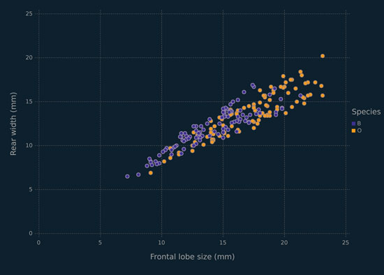
The crabs data are available in the MASS library for R. Therein are five morphological measurements (Table 1.4) on two species of crabs (blue and orange), further separated into two sexes. The variables are highly correlated (e.g., Figures 1.2, 1.3, 1.4). As noted in Table 1.1, these data can be regarded as having two or four classes. The two classes can be taken as corresponding to either species (Figure 1.2) or sex (Figure 1.3), and the four-class solution considers both species and sex (Figure 1.4). Regardless of how the classes are broken down, these data represent a difficult clustering problem — see Figures 1.2, 1.3, 1.4 and consult McNicholas (2016a) for discussion. These data are pre-cleaned.
Table 1.4 The five morphological measurements given in the crabs data, all measured in mm.
Frontal lobe size |
Rear width |
Carapace length |
Carapace width |
Body depth |
Figure 1.2 Scatterplot for rear width versus frontal lobe, for the crabs data, coloured by species.
The food dataset is available from www.kaggle.com and contains data on food choices and preferences for 126 students from Mercyhurst University in Erie, Pennsylvania. The variables in the food data are described in Tables B.1–B.1 (Appendix B). Note that these data are raw, i.e., not pre-cleaned.
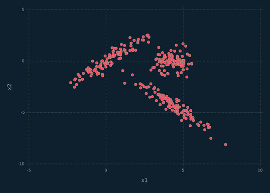
The x2 data are available in the mixture library for R. The data consist of 300 bivariate points coming, in equal proportions, from one of three Gaussian components (Figure 1.5). These data have been used to demonstrate clustering techniques (see, e.g., McNicholas, 2016a).
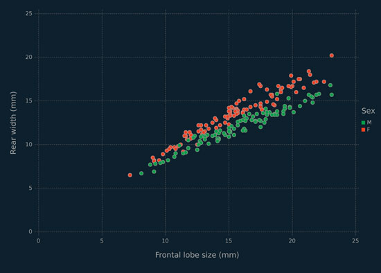
Figure 1.3 Scatterplot for rear width versus frontal lobe, for the crabs data, coloured by sex.
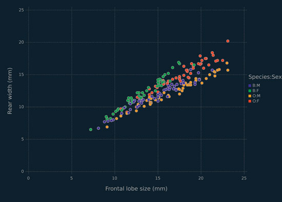
Figure 1.4 Scatterplot for rear width versus frontal lobe, for the crabs data, coloured by species and sex.
Figure 1.5 Scatterplot depicting the x2 data.
The iris data (Anderson, 1935) are available in the datasets library for R. The data consists of four measurements (Table 1.5) for 150 irises, made up of 50 each from the species setosa, versicolor, and virginica. These data are pre-cleaned.
Table 1.5 The four measurements taken for the iris data, all measured in cm.
Sepal length |
Sepal width |
Petal length |
Petal width |
1.6 OUTLINE OF THE CONTENTS OF THIS MONOGRAPH
The contents of this monograph proceed as follows. Several core Julia topics are described in Chapter 2, including variable names, types, data structures, control flow, and functions. Various tools needed for working with, or handling, data are discussed in Chapters 3, including dataframes and input-output (IO). Data visualization, a crucially important topic in data science, is discussed in Chapter 4. Selected supervised learning techniques are discussed in Chapter 5, including K-nearest neighbours classification, classification and regression trees, and gradient boosting. Unsupervised learning follows (Chapter 6), where k-means clustering is discussed along with probabilistic principal components analyzers and mixtures thereof. The final chapter (Chapter 7) draws together Julia with R, principally by explaining how R code can be run from within Julia, thereby allowing R functions to be called from within Julia. Chapter 7 also illustrates further supervised and unsupervised learning techniques, building on the contents of Chapters 5 and 6. Five appendices are included. As already mentioned, the Julia and R packages used herein are detailed in Appendix A, and variables in the food data are described in Appendix B. Appendix C provides details of some mathematics that are useful for understanding some of the topics covered in Chapter 6. In Appendix D, we provide some helpful performance tips for coding in Julia and, in Appendix E, a list of linear algebra functions in Julia is provided.