Chapter 9
Free-radical Addition (Chain-Growth) Polymerization
9.1 Introduction
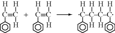
One of the most important types of addition polymerization is initiated by the action of free-radicals, electrically neutral species with an unshared electron. Free-radicals are highly reactive and these types of polymerizations begin with the formation of free-radicals by an initiation reaction. In the developments to follow, a dot (·) will represent a single electron or free-radical. The single bond, a pair of shared electrons, will be denoted by a double dot (:) or, where it is not necessary to indicate electronic configurations, by the usual covalent bond sign (–). A double bond, two shared electron pairs, is indicated by :: or =.
Free-radicals for the initiation of addition polymerization are usually generated by the breakdown of a chemical initiator. These initiators are classified by the method used to catalyze the breakdown: thermal initiators, redox initiators, or photo initiators.
Thermal initiators form free-radicals by the thermal decomposition of compounds such as organic peroxides or azo compounds. Two common examples of thermal initiators are benzoyl peroxide and azobisisobutyronitrile:
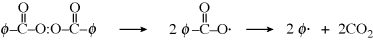
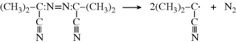
To start these reactions, moderately high temperatures (70–100 °C) are needed.
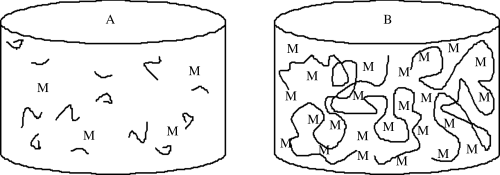
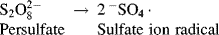
Redox initiators form free-radicals by an oxidation–reduction reaction using chemicals such as ammonium persulfate, usually in combination with an accelerator, such as N,N,N′,N′-tetramethyl ethylene diamine. These reactions can begin a polymerization at lower temperatures. Photo initiators are used less frequently, but can form free-radicals upon exposure to (usually) ultraviolet light. In each case, one initiator molecule forms two free-radicals, often with the formation of a gas. Once the free-radical is formed from the initiator, the polymerization can begin.In contrast to step-growth polymerizations, where condensation can occur between two units of any chain length, addition polymerizations add monomers one at a time to a growing polymer chain (Figure 9.1). This has an important consequence for forming large chains: in addition polymerizations, at any given time during the reaction, the remaining monomer can be easily separated (by evaporation), leaving behind high molecular weight polymers that are mechanically useful (even at somewhat low conversions); recall that for step-growth polymers, conversions topping 99% are required to get even moderate molecular weight materials.
Figure 9.1 Comparison of reactor contents at 50% conversion (a) step-growth or condensation polymerization and (b) addition (or free-radical) polymerization. M = monomer.
9.2 Mechanism of Polymerization
The initiator molecule, represented in a generic sense by I, undergoes a first-order decomposition with a rate constant kd to give two free-radicals, 2 R·:
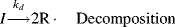
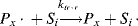
This reaction has a rate constant kd. The radical then adds a monomer by grabbing an electron from the electron-rich double bond, forming a single (R–C) bond with the monomer, but leaving an unshared electron at the other end:
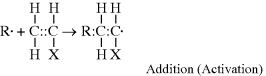
This may be abbreviated by
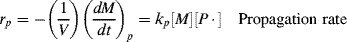
where M is the monomer, and P1· represents a growing polymer with a single repeat unit with a free-radical attached to the other carbon that used to be part of the double bond. The rate constant for addition is ka. Note that the initiator radical actually combines with the monomer, so when a polymer is formed by this method, the end group is normally different from the normal repeat units of the polymer. Fortunately, due to the large size of most polymers, the end group supplied by the initiator is normally insignificant and is usually ignored. The other important thing to notice from Equation (9.2) is that the product of the addition reaction is still a free-radical; thus, it proceeds to propagate the chain by adding another monomer unit:
again maintaining the unshared electron at the chain end, which adds another monomer unit:
and so on. In general, this propagation step is written as
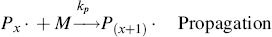
where kp is the rate constant for the propagation step. We have again assumed that reactivity is independent of chain length by using the same kp for each propagation reaction.
The chains continue to grow as long as monomers continue to be available and accessible in the reaction mixture. The reaction ends by a termination step using one of two methods. Two chains can bump together and stick, with their unshared electrons combining to form a single bond between them (combination):
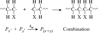
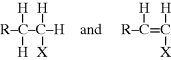
where P(x+y) is a dead polymer chain of (x + y) repeating units. Or, one can abstract a proton from the penultimate carbon on the other forming two dead chains with lengths x and y (disproportionation):
(9.4b) 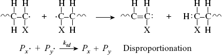
The relative proportion of each termination mode depends on the particular polymer and the reaction temperature, but in most cases, one or the other predominates. Note that another potential method for terminating a polymerization reaction is by chain transfer, where the free-radical is transferred to another species in the reaction mixture, such as a solvent, as discussed in Section 9.6.
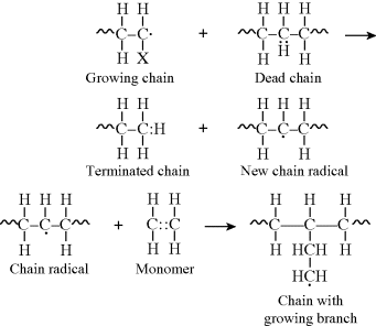
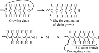
9.3 Gelation in Addition Polymerization
A significant portion of Chapter 8 was devoted to describing gelation and the formation of network polymers by step-growth polymerization, including the gel point conversion, αc, for such reactions. In free-radical polymerizations, all monomers have the same reactive functional group (the alkene double bond). Monomers that have only one C=C produce linear polymers, but those with two or more alkenes normally result in branch points and the formation of crosslinked networks. Such multifunctional monomers are termed crosslinking agents, and need only be added at 1 mol% (or even less) to successfully form a network. Because free-radical polymers add monomers to long growing chains, these crosslinking agents are added just as the other monomers and begin to form crosslinked networks, even at low conversions (particularly if the amount of crosslinking agent is high). The three-part mechanism (initiation, propagation, and termination) is largely the same as above. The most important parameters in determining the structure of these polymers are the fraction of crosslinking agents added and their functionality (number of double bonds). The resulting structures are characterized by  , the molecular weight between crosslinks. Lightly crosslinked gels will swell appreciably in a good solvent, while those made with high concentrations of crosslinking agents are often brittle and easily crack. Because a gel point conversion is much less important for networks made by free-radical polymerization, no further discussion is included in this chapter.
9.4 Kinetics of Homogeneous Polymerization
Free-radical polymerizations can take place in either homogeneous (single phase) or heterogeneous (multiple phase) mixtures. In this section, we will consider only homogeneous reactions, where the monomer is either reacted in bulk or a good solvent is used so that the monomer, initiator, and polymers of all lengths are soluble in a single phase. To determine the rate of polymerization, we must consider the rates of each of the steps (initiation, addition, propagation, and termination) involved in the mechanism.
In practice, not all the radicals generated in Equation (9.1) actually initiate chain growth as in Reaction (9.2). Some recombine through the reverse reactions, or others are used up by side reactions. Thus, f, the fraction of radicals generated in the initiation step that actually initiate chain growth through Reactions 9.1 and 9.2, is important in developing rate equations:
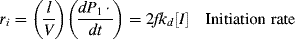
where V is the volume of the reaction mass, P1· is the moles of chain radicals with x = 1, and [I] is the initiator concentration (moles/volume). In the notation used here, the quantity Q of a species without brackets represents the moles of the species and when enclosed in square brackets, [Q], the molar concentration of the species. They are related by

Although it is rarely mentioned explicitly, Equation (9.5) is based on the generally valid assumption that the rate of Reaction (9.2) is much greater than that of Reaction (9.1), that is, the initiator decomposition is rate controlling. Thus, as soon as an initiator radical is formed, it grabs a monomer molecule, starting chain growth, so ka does not appear in the rate expression.
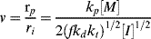
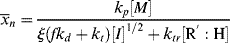
According to Reaction (9.3), the rate of monomer removal in the propagation step is
where M is the moles of monomer and [P·] is the total concentration of growing chain radicals of all lengths:
(9.8) 
The rate of removal of chain radicals is the sum of the rates of the two termination reactions. Since both are second order
(9.9) 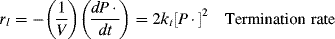
where the termination rate constant, kt, adds the rate constants for termination by combination (ktc) and by disproportionation (ktd):
(9.10) 
Unfortunately, the unknown quantity [P·] is present in the equations. It cannot be measured during a reaction, but can be removed from the equations by making the standard kinetic assumption of a steady-state concentration of a transient species, in this case, the chain radicals, such that d[P·]/dt = 0 during the reaction. For [P·] to remain constant, chain radicals must be generated at the same rate at which they are removed. Thus, we assume that the rates of initiation and termination must be equal (ri = rt), or
(9.11) 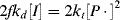
This gives the chain-radical concentration as
which, when inserted into Equation (9.7) provides an expression for the rate of monomer consumption in the propagation reaction:

One molecule of monomer is consumed in the addition step (Eq. (9.2)) also, but for long chains this is insignificant, so that Equation (9.13) may be taken as the overall rate of polymerization, the rate at which monomer is converted to polymer.
Equation (9.13) is the classical rate expression for a homogeneous, free-radical polymerization. It has been an extremely useful approximation over the years, particularly in fairly dilute solutions, but deviations from it are sometimes observed. It is now evident that many deviations are due to the fact that the termination reaction is diffusion controlled, so kt is not really a constant but decreases in time as the polymerization proceeds. In certain cases of practical interest, these deviations can be of major significance. They are discussed in Chapter 12 on polymerization practice.
It is often more convenient to work in terms of monomer conversion X. By making use of the definition of conversion:

and Equation (9.6) for M, we can rewrite Equation (9.13) as

Note that the conversion X used here is a very different quantity than the p used in Chapter 8 for step-growth polymers. Here, X is the fraction of monomer molecules that have reacted to form polymer. The quantity p represents the fraction of functional groups that have reacted (whether on a monomer or part of a growing polymer chain). In step-growth polymerization, each monomer molecule has several functional groups that react independently, so p is not the fraction of reacted monomer. (Compare to free-radical addition, where both sides of the double bond are reacted in sequence.)
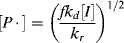
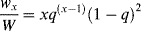
Integration of Equation (9.13a) gives conversion as a function of time. A form occasionally used in studying the initial stages of an isothermal, batch reaction is obtained by assuming a constant initiator concentration [I]o with the initial condition X = 0 at t = 0:
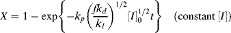
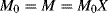
The assumption of constant [I] may not be realistic at high conversions for two reasons. First, the initiator concentration can decrease significantly with time. Second, the volume of the reaction mass will, in general, change with conversion. Most liquid-phase addition polymerizations undergo a density increase of 10–20% from pure monomer (X = 0) to polymer (X = 1) (carrying out the reaction in an inert solvent reduces this, of course).
We can include the first-order initiator decay:
(9.16a) 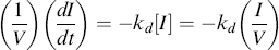
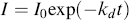
and integrate from t = 0 with I = Io to get
We then assume that the volume of the reaction mass is linear with conversion, as outlined by Levenspiel [1]:
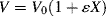
where ε is the fractional change in volume from X = 0 to X = 1 and Vo is the volume of the reaction mass at X = 0. Combining Equations (9.6) (for I), (9.13), (9.16b), and (9.17) gives
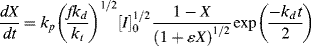
The variables in Equation (9.18) may be separated and it may be integrated analytically with respect to time, at least, to give
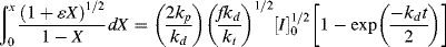
Unfortunately, the left side of Equation (9.19) cannot be integrated analytically by normal human beings. An explicit expression for X as a function of t is extremely difficult to determine, so calculation of X(t) is normally done by numerical or by computational methods.
If we can neglect volume change (ε = 0), we can solve the integral explicitly to get

This expression has some interesting and important implications when compared with Equation (9.15). Setting t = ∞ reveals that there is a maximum attainable conversion that depends on [I]o:
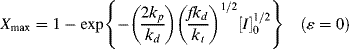
This “dead-stop” situation is basically a matter of the initiator being used up before the monomer, but it is not revealed by Equation (9.15), which always predicts complete conversion in the limit of infinite time. Thus, the use of Equation (9.15) instead of Equation (9.19) or (9.20) can result in considerable error at high conversions, although the results approach one another at low conversions.
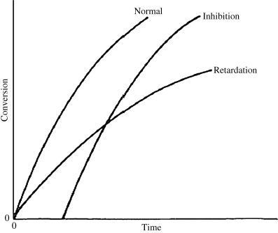
Side reactions cause deviations from the classical kinetics. Agents that cause these reactions are generally categorized as inhibitors or retarders (though accelerators can also be used). An inhibitor delays the start of the reaction, but once begun, the reaction proceeds at the normal rate. Liquid vinyl monomers are usually shipped with a few parts per million of inhibitor to prevent polymerization in transit. A retarder slows down the reaction rate, which can be used to allow a reacting mixture to be worked with before setting. Some chemicals combine both effects. These are illustrated in Figure 9.3. Oxygen is a free-radical scavenger, so it behaves as an inhibitor for free-radical polymerization; thus, these reactions are normally carried out under a blanket of nitrogen.
Figure 9.2 Conversion versus time for an isothermal, free-radical batch polymerization (data of Example 9.2): Equation (9.15), [I] = constant; Equation (9.19),  = −0.136; Equation (9.20), = 0.
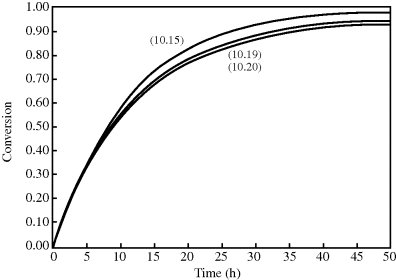
Figure 9.3 Change in reaction behavior due to inhibitor or retarder.
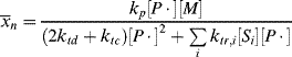
9.5 Instantaneous Average Chain Lengths
As in step-growth polymerization, a distribution of chain lengths is always obtained in a free-radical addition polymerization because of the inherently random nature of the termination reaction with regard to chain length. Expressions for the number-average chain length are usually couched in terms of the kinetic chain length, ν, which is the rate of monomer addition to growing chains over the rate at which chains are started by initiator radicals, that is, the average number of monomer units per growing chain radical at a particular instant.1 It thus expresses the efficiency of the initiator radicals in polymerizing the monomer:
If the growing chains terminate exclusively by disproportionation, they undergo no change in length in the process, but if combination is the exclusive mode of termination, the growing chains, on average, double in length upon termination. Therefore,
(9.23a) 
(9.23b) 
The average chain length may be expressed more generally in terms of a quantity ξ, the average number of dead chains produced per termination reaction, which equals the ratio of the rate of dead chain formation to the rate of termination reactions. Since each disproportionation reaction produces two dead chains and each combination one,
(9.24) 
(9.25) 

The instantaneous number-average chain length is the rate of addition of monomer units to all chains (rp) over the rate of dead chain formation:
When ktd  ktc, ξ = 2, and when ktc
  ktd, ξ = 1, duplicating the previous result, but Equation (9.27a) can also handle various degrees of mixed termination.
Keeping in mind that  is one of the most important factors in determining certain mechanical properties of polymers, what is the significance of Equation (9.27a) A growing chain may react with another growing chain and terminate, or it may add another monomer unit and continue its growth. The more monomer molecules that are in the vicinity of the chain radical, the higher the probability of another monomer addition, hence the proportionality to [M]. On the other hand, the more initiator radicals that are present competing for the available monomer, the shorter the chains will be, on an average, causing the inverse proportionality to the square root of [I]. Equation (9.13) shows that the rate of polymerization can be increased (always an economically desirable goal) by increasing both [M] and [I], the former being more efficient than the latter. However, there is an upper limit to [M] set by the density of the pure monomer at the reaction conditions. So it is often tempting to increase [I] to attain higher rates. But according to Equation (9.27a), this unavoidably lowers
  . You cannot have your cake and eat it, too.
9.6 Temperature Dependence of Rate and Chain Length
We may assume that the temperature dependence of the individual rate constants in each of the steps of the reaction are given by the Arrhenius expression:
(9.28) 
where ki is the rate constant for a particular elementary reaction, Ai is its frequency factor, and Ei is its activation energy. This expression is common in chemical kinetics, and results in the rule of thumb that for every 10 °C increase in temperature, the rate approximately doubles (which holds for temperatures around 300 K). Because most addition polymerizations are exothermic, the temperature of the reaction mixture increases during the polymerization, which causes an increase in the kinetic rate constants, which raises the temperature even faster, and so on, causing a run-away reaction. This behavior is related to the Tromsdorff effect, whereby chain termination occurs more quickly than expected, leading to lower molecular weight chains. This subject is covered in more detail in Chapter 12, Polymerization Practice.
If we neglect the temperature dependence of f, Equation (9.13) becomes
(9.29) 
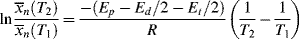
where C combines temperature-independent quantities into a single constant and Ep +Ed/2 − Et/2 is the effective activation energy for polymerization. Therefore, between two (absolute) temperatures T1 and T2:
Similar treatment of Equation (9.27a), with the assumption that ξ is independent of temperature, results in:
where Ep − Ed/2 − Et/2 is the effective activation energy for the number-average chain length.
 for a typical homogeneous, free-radical addition polymerization when the temperature is raised from 60 to 70 °C.
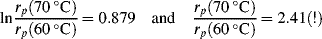
 is −10 kcal/mol. With Equation (9.31), we get
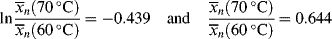
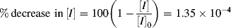
 is subject to a 35.6% decrease over the same temperature range.
9.7 Chain Transfer and Reaction Inhibitors
In practice, another type of reaction sometimes occurs in free-radical addition polymerizations. These chain-transfer reactions kill a growing chain radical and can start a new one in its place (as long as the radical transfers to another monomer):
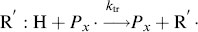
(9.32b) 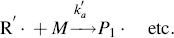
Thus, chain transfer results in shorter chains, and if the reactions in Equation (9.32a) are not too frequent compared to the propagation reaction and do not have very low rate constants, chain transfer will not change the overall rate of polymerization appreciably.
The compound R′:H in the above reaction is known as a chain-transfer agent. They are also sometimes referred to as chain terminating agents, because the free-radical on the growing polymer Px is removed. Under appropriate conditions, almost anything in the reaction mass may act as a chain-transfer agent, including initiator, monomer, solvent, and dead polymer.
Reaction inhibitors can also change the polymerization rate. Inhibitors for addition polymerizations are typically free-radical scavengers—chemicals that can gobble up free-radicals quickly and prevent or slow the initiation and propagation steps of the polymerization mechanism. Oxygen is one such scavenger, and in some addition polymerizations, even oxygen dissolved in the reaction mixture must be removed to obtain appreciable molecular weight polymers. Other inhibitors are often added to monomers being shipped so that they do not autopolymerize before a reaction is desired. Quinone-type chemicals are often used in this capacity.
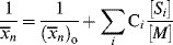
Most frequently, mercaptans (also known as thiols), the sulfur analogs of alcohols (R′S:H), are added to the reaction mass as effective chain-transfer agents to lower the average chain length.
The rate of dead chain formation by chain transfer
must be added to the denominator of Equation (9.27a) to give the total rate of dead chain formation:
(9.34) 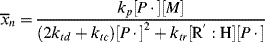
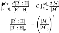
Using Equations (9.12) and (9.26) gives
Taking the reciprocal of Equation (9.35) gives
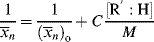
where C is the chain-transfer constant = ktr/kp and  is simply the average chain length in the absence of chain transfer from Equation (9.27a). Thus, a plot of
  versus [R′:H]/[M] is linear with a slope of C and intercept of
  .
.


9.8 Instantaneous Distributions in Free-Radical Addition Polymerization
A growing polymer chain Px· can either propagate, terminate, or transfer. The propagation probability, q, is the probability that it will propagate rather than transfer or terminate and is given by
(9.38) 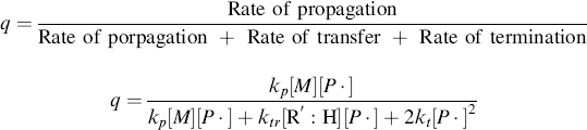
which becomes, with the aid of Equation (9.12),
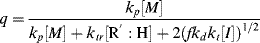
To get chain-length distributions from q, we must separately consider termination by disproportionation and combination because the two mechanisms give rise to different distributions. First, consider only those chains whose growth is terminated by either disproportionation (kt = ktd, ξ = 2) or chain transfer. The resulting distributions are the same, because a growing chain does not know if it has been killed by an encounter with another growing chain or with a chain-transfer agent. Either way, its growth stops with no change in length (that is not the case for combination). By taking the reciprocal of Equation (9.39), we get
(9.40) 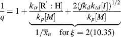
Therefore,

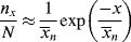
Now, a polymer molecule containing x units, Px, has been formed by x − 1 propagation steps (the remaining unit was incorporated in the addition step), each with a probability q, and one disproportionation or transfer step with a probability 1 − q. The probability of finding such a molecule is equal to its number (mole) fraction; therefore,
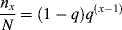
which, lo and behold, is the “most probable” distribution (Eq. (8.3)) again. But, although Equations (9.42) and (8.3) appear the same, p and q are totally different quantities. In batch step-growth polymerization, p increases monotonically from 0 to 1 as the reaction proceeds. In free-radical addition polymerization, however, q depends only indirectly on conversion, since [I], [M], and [R′:H] will, in general, vary with conversion. In the usual case, q is always close to 1, as indeed it must be to form high molecular weight polymer chains.

This points out another important difference between the seemingly similar Equations (9.42) and 8.3. The distributions for free-radical addition include only terminated chains, not unreacted monomer. In a step-growth reaction, there are no terminated chains short of complete conversion, and x = 1 in Equation 8.3 represents unreacted monomer.
Note that by analogy to Equation (8.6),  for the most-probable distribution should be

which is greater by one than the value given by Equation (9.41). This discrepancy arises from the fact that the kinetic derivation of Equation (9.41) neglects the monomer molecule added to the chain in the addition step, while that molecule is specifically considered in the derivation of Equation (9.42). From a practical standpoint, this makes little difference, because in the usual free-radical addition polymerization, q → 1 and  »
» 1.
1.
By analogy to Equations (8.9)–(8.11) for step-growth polymerization:
(9.45) 

Here, however, unlike the case in step growth, the approximations q → 1 and  » 1, and ln q ≈ q − 1 are almost always applicable, and Equations (9.42), (9.44), and (9.46) simplify to (recall Example 5.5)

Now, let us consider chains that exclusively terminate by combination (kt = ktc; ξ = 1):
(9.50) 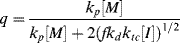
(9.51) 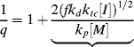
(9.27b) 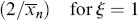
from which

A dead chain consisting of x units is formed by the combination of two growing chains, one containing y units and the other containing x − y units:
(9.53) 
One growing chain has undergone y − 1 propagation steps, each of probability q. The other chain has undergone x − y − 1 propagation steps, each of probability q. Two growing chains are terminated, each with a probability of 1 − q. But, each dead chain consisting of x total units could have been formed in x − 1 different ways; for example,
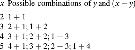
and all possible ways to form a chain of x units total must be counted. Therefore,
(9.54) 
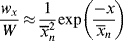
For this distribution,

which is greater by two than the value given by Equation (9.52), since the first monomer incorporated in the addition step is now considered for each of the chains, and
(9.56) 
(9.57) 
For the usual free-radical case, where q → 1,  » 1, and ln q ≈ q − 1:

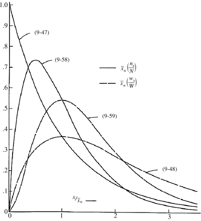
These distributions are plotted in reduced form in Figure 9.4. Note that termination by combination sharpens the distributions because of the low probability of two very short or two very long macroradicals combining.
Figure 9.4 Instantaneous number- and weight-fraction distributions of chain lengths in free-radical addition polymerization. Equations (9.47) and (9.48) are for termination by disproportionation and/or chain transfer; Equations (9.58) and (9.59) are for termination by combination.
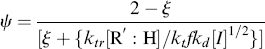
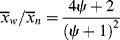
As shown above, chains terminated by combination follow a different distribution than those terminated by disproportionation or chain transfer. If a material contains chains formed according to both distributions (as would happen, e.g., if a chain-transfer agent were added to a system that terminates inherently by combination), the distributions must be summed according to the proportion (mole or mass fraction) of each, as detailed in Kenat et al. [2] To solve this situation, let ψ be the mole (or number) fraction of the chains that have been terminated by combination. The weight fraction of chains terminated by combination is 2 ψ/(ψ + 1). In terms of kinetic parameters, ψ is given by
where ξ is defined by Equation (9.26). In terms of ψ, the general distributions become


For termination entirely disproportionation and/or chain transfer, ψ = 0 and Equations (9.62), (9.63), (9.64) reduce to Equations (9.42), (9.43)–(9.49); for termination exclusively by combination, ψ = 1, they reduce to Equations (9.58)–(9.60), but these new equations are also able to describe various degrees of mixed termination.
 for the styrene polymerization in Example 9.1 for conditions at the start of the reaction. Neglect chain transfer. Styrene terminates by combination at 60 °C so that kt = ktc (ξ = 1). [M]o = 8.72 mol/L.
 = 434 (
 = 45,200), so we are getting high molecular weight polymer right off the bat, too.
9.9 Instantaneous Quantities
It is obvious from Equation (9.13) that the rate of polymerization is an instantaneous quantity; it depends on the particular values of [M], [I], and T (through the temperature dependence of the rate constants) that exist as a particular instant (and location, for that matter) in a reactor. In a uniform, isothermal batch reaction (Example 9.1), the rate of polymerization decreases monotonically because of the decreases in both [M] and [I] with time. In a similar fashion,  according to Equation (9.35) is a function of [M], [I], T, and [R′:H], all of which may vary with time (and/or location) in a reactor. But is the concept of an instantaneous
  valid? How much do these quantities change during the lifetimes of individual chains? This important point is clarified in the following example.
 , and compare it with the half lives of monomer and initiator,
 ,
, , and
, and
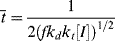
 = 0.141 s (!). From Figure 9.1, the time to reach 50% conversion (monomer half life) is about 8 h. From equation (9.16b), the time to reach (I/Io) = 0.5 is −(ln 0.5)/kd or 20 h.

 = 0.141/ s, X = 3.36 × 10⁻⁶ of 3.36 × 10⁻⁴%.
Some important conclusions can be drawn from the preceding example. In a typical, homogeneous, free-radical addition polymerization, there are lots of chains growing at any instant. The average lifetime of a growing chain, however, is extremely short, many orders of magnitude smaller than the half-lives of either monomer or initiator. Once a chain has been initiated by the decomposition of an initiator molecule (recall that this is the slow step), it grows and dies in a flash, and once terminated, it plays no further role in the reaction (unless it happens to act as a chain-transfer agent, as in Example 9.6) and merely sits around inertly as more chains are formed. This is to be contrasted with step-growth polymerization, in which the chains always maintain their terminal reactivity and continue to grow throughout the reaction (see Table 9.1).
Table 9.1 Comparison of Step-Growth (Chapter 8) and Addition (Chapter 9) Polymerizations.
| Characteristic | Step-Growth Polymerization | Addition Polymerization |
| Typical monomer structure | Bifunctional monomers with two organic functional groups (amines, alcohols, acids, etc.) | Monomers have a polymerizable double bond (such as in vinyl or acrylate monomers) |
| Reactor contents during polymerization at 50% conversion | p = .5; 50% of functional groups reacted,  = 2. Only small chains present. = 2. Only small chains present. |
X = 0.5; large polymer chains and monomer are in the reactor,  depends on initiator concentration depends on initiator concentration |
| Reaction speed (kinetics) | Generally slow; depends on reactivity of functional groups; dimers, trimers, etc., start to form from the start, making the solution syrupy and viscous. | Generally fast; solution contains primarily monomers until high conversions are reached, so the solution retains relatively low viscosity |
| Initiator required | No | Usually |
| Effect of temperature | Arrhenius behavior | Arrhenius behavior |
| Networks and gels | Requires tri- (or higher) functional monomers (A3) and high enough conversions to exceed the critical gelation point. | Multiple polymerizable double bonds on a monomer result in network structures; a gel starts to form as soon as reaction propagates (even at low conversion) |
The lifetime of free-radical chains is, in fact, so short that changes in concentrations are entirely negligible during a chain lifetime. Hence, it is perfectly proper to characterize chains formed at any instant when [M], [I], T, and [R′:H] have a particular set of values. All the quantities defined to this point ( ,
,  , q) and, therefore, the distributions are just such instantaneous quantities. For this reason, it was necessary to specify conditions “at the start of the reaction” in earlier examples to permit their calculations.
9.10 Cumulative Quantities
Unfortunately (for the sake of simplicity), as conditions vary within a polymerization reactor, so do the instantaneous quantities, making it very difficult to accurately determine  and
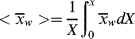
and  as functions of time. The polymer in the reactor is a mixture of material formed under varying conditions of temperature and concentrations, and therefore must be characterized by cumulative quantities, which are integrated averages of the instantaneous quantities of the material formed up until the reactor is sampled. The cumulative number-average chain length, <
 >, is simply the total moles of monomer polymerized over the total moles of dead chains formed. In a batch reactor, for example,


(For termination by disproportionation, each successful initiator reaction results in two dead chains, and for combination, one; hence, the need for ξ. Each reacted molecule of chain-transfer agent results in one dead chain.) Therefore,
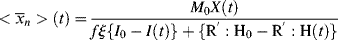
(If you wish to neglect volume change, all the molar quantities can be enclosed in square brackets to give concentrations.) Note that the preceding expression is indeterminate at t = 0. At this point, however,  = <
= < > = 1 (just monomers), both are given by Equation (9.35).
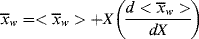
A good analogy for visualizing the relation between  and <
and < > is the “well-stirred, adiabatic bathtub.”
  corresponds to the temperature of the water leaving the tap, and <
 > to the temperature of the water in the tub. So, the newly formed polymer entering from the top must be averaged with all that is been made earlier (the stuff already in the bathtub). As long as the tub is not full, the analogy applies to a batch reactor. If the tub is allowed to fill and overflow, it applies to a continuous stirred-tank reactor as well.
 and <
and < > versus X.
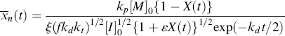
 , and <
 > to t through Equations (9.19) or (9.20), (9.27′) and (9.65′).
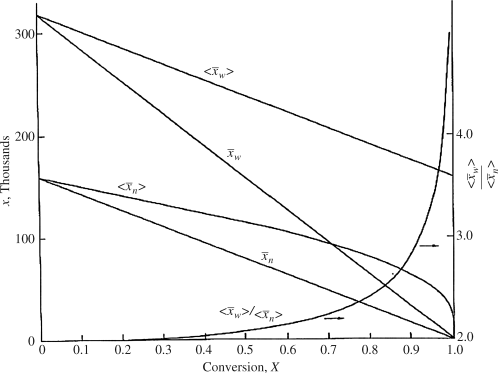
 goes through a minimum at high conversions. In fact, it ultimately goes to infinity, because in this example of “dead-stop” polymerization, [I] goes to zero while [M] remains finite. Not so obvious on this scale is the fact that <
 > must also go through a minimum. As long as
  is less than <
 >, the former will continue to drag the latter down (adding colder water from the tap cools off the water in the tub). When
  is greater, it must pull <
 > up (you warm up the water in the tub by adding hotter water from the tap). Therefore, there must be a minimum in <
 > where the two curves cross, although <
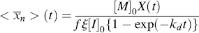
 > does reach a finite value of 173.5 at the maximum conversion of 99.48%. (The numbers quoted apply for ξ = −0.136. For ξ = 0, they are 173.2 and 99.30%.) Even though the last tiny drop from the tap may be very hot, it is not going to significantly raise the temperature of the 50 gallons already in the tub.
Figure 9.5 Instantaneous and cumulative number-average chain lengths versus conversion for an isothermal, free-radical, batch polymerization (data of Example 9.27′).
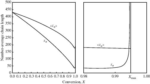
It is instructive to compare the results of Example 9.27′ with Equation 8.6 for step-growth polymerization. There,  increases monotonically with conversion (p), and high conversions are necessary for high chain lengths. This is not true for free-radical addition, where chains formed early in the reaction have fully developed chain lengths.
Also keep in mind that if samples are removed from the reactor and analyzed for number-average chain length, the quantity determined is < >. The cumulative quantity is what characterizes the reactor contents. The only way to measure
  would be to sample at a very low conversion, where
  ≈ <
≈ < >.
>.
9.11 Relations Between Instantaneous and Cumulative Average Chain Lengths for A Batch Reactor
Given any instantaneous or cumulative average chain length as a function of conversion in a batch reactor, the others may be calculated as follows. Recall that conversion is defined as
(9.14) 
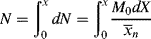
The moles of monomer polymerized up to conversion X is
while the moles of monomer polymerized in a conversion increment dX is

The moles of polymer chains formed in the conversion increment dX is:

The total moles of polymer chains formed up to conversion X is obtained by integrating dN:
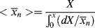
But, by definition of < >, N is also given by

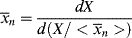
Equating the two expressions for N gives
Differentiating Equation 10.66 reverses the result:
Equation 5.6 gives the weight average of a mixture in terms of a summation of the weight averages of the finite components of the mixture. For a mixture of differential components of weight-average chain length  , this may be generalized to
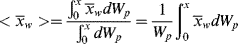
where
dWp = weight of polymer formed in conversion increment of dX and
Wp = total weight of polymer formed up to conversion X.
Now Wp = WoX and dWp = WodX, where Wo is the weight of monomer fed; so
and by differentiating Equation (9.68), we get
The relation between  and
and  is, of course, determined on a microscopic scale by the nature of the instantaneous distribution, which fixes the instantaneous polydispersity index,
  /
/ , given by Equation (9.64). However, it is not the instantaneous polydispersity index that characterizes the reactor product but rather the cumulative polydispersity index <
 >/<
>/< >. Even though the instantaneous polydispersity index may remain constant, if the instantaneous averages vary during the reaction (as in Example 9.27′), the cumulative distribution must be broader than the instantaneous, increasing the cumulative polydispersity index (Example 5.2 provides a simple quantitative illustration of this). This is one of the reasons why commercial polymers often have polydispersity indices much greater than the minimum value given by Equation (9.64).
The “road map” below summarizes how to get between the various averages when one is known as a function of conversion:
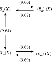
Remember that < > and <
 > can be experimentally determined by sampling the reactor, but
  and
and  can be obtained only by calculation at finite conversions.
 is too. This will give the narrowest possible distribution, due only to the microscopically random nature of the reaction. With an ideal CSTR, <
 >/<
>/< > =
> =  /
/ . In a batch reactor, [M] and [I] decrease as the polymers are produced. In both of the tubular reactors, where the reaction occurs as the reactants flow through a tube, the [M] decreases as the reacting mixture moves from the inlet to the exit. In each of the latter three reactors,
  changes with conversion, broadening the distribution so that {<
 >/<
>/< >} >
>} >  /
/ . Note that changes in temperature (which are not uncommon for exothermic polymerizations) can cause the rate constants to vary, and thus also contribute to broadening of the distribution.
 and kd = 4.369 × 10⁻⁷/s−1. This particular polymer terminates by disproportionation (ξ = 2). Neglect chain transfer. Assume perfect reactor stirring and f = 1. Because this reaction is carried out in a rather dilute solution, volume change is negligible. Calculate and plot
  , <
, < >,
>,  , <
, < >, and <
 >/<
>/< > versus conversion for this system.
 is very large and kd is small (compare with Example 9.1.). This has some important consequences. First, the chain lengths will be tremendous. (Although this example is based on a real system, in real life it is likely that chain lengths would be transfer limited, that is, the chains would transfer to something in the reaction mass before reaching the lengths calculated.) Second, [I] remains essentially constant throughout the course of the reaction. As a result,
  is linear with X (combine Equations (9.27a) and (9.14) to see why). This, in turn, allows easy analytical evaluation of Equations (9.66), (9.67), (9.68), (9.69), but also renders Equation (9.65) useless.
 = 2
= 2 , so that

Figure 9.6 Instantaneous and cumulative number- and weight-average chain lengths and the cumulative polydispersity index for an isothermal, free-radical, batch polymerization (Example 9.12).
If it is necessary to maintain minimum polydispersity (albeit with shorter chains), the drift in instantaneous chain length can often be compensated for by varying the rate of addition of chain-transfer agent to the reactor. In Example 9.12, a high initial rate of a very active agent could be reduced as conversion increased, thereby counteracting the decrease in  (and increase in polydispersity) that would otherwise occur. Adjusting the rate of addition of chain-transfer agent to maintain
  constant has been discussed for batch [3] and continuous [2] reactors.
Example 9.12 constitutes one of the simplest possible illustrations of what is sometimes termed “polymer reaction engineering.” Even a minor complication, such as substitution of the parameters of Example 9.1. or the inclusion of chain transfer would necessitate a numerical solution. While the basic principles are there, additional detail is beyond the scope of this chapter, but you might wish to consider the application of these principles to a nonisothermal reactor, etc.
9.12 Emulsion Polymerization
The preceding discussion of free-radical addition polymerization has considered only homogeneous reactions. Considerable polymer is produced commercially by a complex heterogeneous free-radical addition process known as emulsion polymerization. This process was developed in the United States during World War II to manufacture synthetic rubber. A rational explanation of the mechanism of emulsion polymerization was proposed by Harkins [4] and quantified by Smith and Ewart [5] after the war, when information gathered at various locations could be freely exchanged. Perhaps the best way to introduce the subject is to list the feed sent to a typical reactor.
| Typical Emulsion Polymerization Feed |
| 100 parts (by weight) monomer (water insoluble) |
| 180 parts water |
| 2–5 parts fatty acid surfactant (emulsifying agent) |
| 0.1–0.5 part water-soluble initiator |
| 0–1 part chain-transfer agent (monomer soluble) |
The surfactant is the critical ingredient that helps to form an emulsion where the monomer is dispersed in droplets. Surfactants are generally the sodium or potassium salts of organic acids or sulfates that have alkane-based R groups:
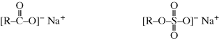
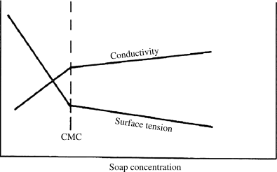
When they are added to water in low concentrations, they ionize and float around freely much as sodium chloride ions would. The anions, however, consist of a highly polar hydrophilic (water-seeking) “head” (COO− or SO3−) and an organic, hydrophobic (water-fearing) “tail” (R). As the surfactant concentration is increased, a value is suddenly reached where the anions begin to agglomerate in micelles rather than float around individually. These micelles have dimensions on the order of 5–6 nm, far too small to be seen with a light microscope (although a successful emulsion of micelles will turn a solution cloudy, as a bottle of oil and vinegar salad dressing would look after shaking). The micelles consist of a tangle of the hydrophobic tails in the interior (getting as far away from the water as possible) with the hydrophilic heads on the outside. This process is easily observed by following the variation of a number of solution properties with surfactant concentration, for example, electrical conductivity or surface tension (see Figure 9.7). The break in the slope occurs when micelles start to form with higher concentrations of surfactant, and is known as the critical micelle concentration or CMC.
Figure 9.7 Variation of solution properties to define the CMC.
When an organic monomer is added to an aqueous micelle solution, it naturally prefers the organic environment within the micelles. Some of it congregates there, swelling the micelles until equilibrium is reached with the contraction force of surface tension. Most of the monomer, however, is distributed in the form of much larger (1 μm or 1000 nm) droplets stabilized by surfactant. This complex mixture is an emulsion. The cleaning action of surfactants is why they are widely used in soaps and detergents, where they emulsify oils and greases.
Despite the fact that most of the monomer is present in the droplets, the swollen micelles, because of their much smaller size, present a much larger surface area than the droplets. This is easily seen by assuming a micelle volume to drop volume ratio of 1/10 and using the ballpark figures given above. Since the surface/volume ratio of a sphere is 3/R,
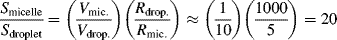
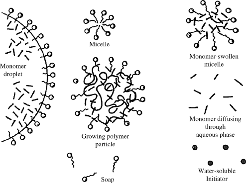
Figure 9.8 illustrates the structures present during emulsion polymerization.
Figure 9.8 Structures in emulsion polymerization.
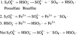
Free-radicals for classical emulsion polymerizations are generated in the aqueous phase by the decomposition of water-soluble initiators, usually potassium or ammonium persulfate:
Redox systems, so called because they involve the alternate oxidation and reduction of a trace catalyst, are one of the alternatives for generating free-radicals in the initiation step. For example,
The original wartime GR-S, poly(butadiene-co-styrene), polymerization was carried out at 50 °C using potassium persulfate initiator (“hot” rubber). The use of the more efficient redox systems allowed a reduction in polymerization temperature to 5 °C (“cold” rubber). The latter has superior properties because the lower polymerization temperature promotes cis-1-4-addition of the butadiene.
The radicals thus generated in the aqueous phase bounce around until they encounter some monomer. Since the surface area presented by the monomer-swollen micelles is so much greater than that of the droplets, the probability of a radical entering a monomer-swollen micelle rather than a droplet is large. As soon as the radical encounters the monomer within the micelle, it initiates polymerization. The conversion of monomer to polymer within the growing micelle lowers the monomer concentration therein, and monomer begins to diffuse from uninitiated micelles and monomer droplets to the growing, polymer-containing micelles. Those monomer-swollen micelles not struck by a radical during the early stages of conversion thus disappear, losing their monomer and surfactant to those that have been initiated. This first phase of the reaction was termed Stage I by Smith and Ewart. The reaction mass now consists of a stable number of growing polymer particles (originally micelles) and the monomer droplets, termed Stage II.
In Stage II, the monomer droplets simply act as reservoirs supplying monomer to the growing polymer particles by diffusion through the water. The monomer concentration in the growing particles maintains a nearly constant dynamic equilibrium value dictated by the tendency toward further dilution (increasing the entropy) and the opposing effect of surface tension attempting to minimize the surface area. Although most organic monomers are normally thought of as being water “insoluble,” their concentrations in the aqueous phase, though small, are sufficient to permit a high enough diffusion flux to maintain the monomer concentration in the polymerizing particles [6]. Smith and Ewart then subdivided Stage II into three subcases where the ratio of growing free-radicals per particle is « ½ (case 1), = ½ (case 2), or » ½ (case 3). The description that follows applies to their case 2 that often happens in practice.
A monomer-swollen micelle that has been struck by a radical contains one growing chain. With only one radical per particle, the chain cannot terminate by disproportionation or by combination, and it continues to grow until a second initiator radical enters the particle. Under conditions prevailing within the particle in case 2 (tiny particles and highly reactive radicals), the rate of termination is much greater than the rate of propagation, so the chain growth is terminated essentially immediately after the entrance of the second initiator radical [6]. The particle then remains dormant until a third initiator radical enters, initiating the growth of a second chain. This second chain grows until it is terminated by the entry of the fourth radical, and so on.
9.13 Kinetics of Emulsion Polymerization in Stage II, Case 2
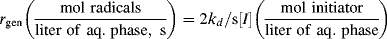
Thus, in Stage II, the reaction mass consists of a stable number of monomer-swollen polymer particles that are the loci of all polymerizations. At any given time (for case 2), a particle contains either one growing chain or no growing chains (assumed to be equally probably). Statistically, then, if there are N particles per liter of reaction mass, there are N/2 growing chains per liter of reaction mass.
The polymerization rate is given, as before, by
(9.7) 
where kp is the usual homogeneous propagation rate constant for polymerization within the particles and [M] is the equilibrium monomer concentration within a particle. Now,
(9.70) 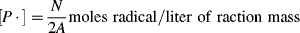
where A is Avogadro's number (6.02 × 10²³ radicals/mol radicals). The rate of polymerization is then

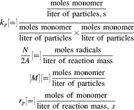
where typical units for the various terms are as follows:
Equation (9.73) thus gives the rate of polymerization per total volume of reaction mass. Surprisingly, it predicts the rate to be independent of initiator concentration. Moreover, since both N and [M] are constant in Stage II, a constant rate is predicted. This is borne out experimentally, as shown in Figure 9.9 [4]. Deviations from linearity are observed at low conversions as N is being stabilized in Stage I, and at high conversions in Stage III, when the monomer droplets are used up and are no longer able to supply the monomer necessary to maintain [M] constant within the growing polymer particles. Thus, in Stage III, the rate drops off as the monomer is exhausted within the particles.
Figure 9.9 The emulsion polymerization of isoprene as a function of surfactant (potassium laureate) concentration—from low (0.01 molar) and slow to high (0.5 molar) and fast. Reprinted from Harkins [4]. Copyright 1947 by the American Chemical Society. Reprinted by permission of the copyright owner.
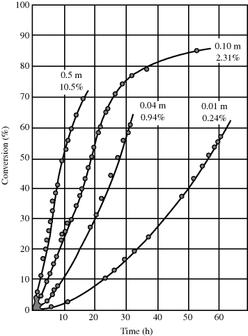
Note that the rate increases with surfactant (emulsifier) concentration! The more surfactant used, the more micelles are established in Stage I, and the higher N will be in Stage II. The predicted independence of rate on initiator concentration must be viewed with caution. It is valid as long as N is held constant, but in practice, N increases with [I]o. The more initiator added at the start of a reaction, the greater the number of monomer-swollen micelles that start growing before N is stabilized. Methods are available for estimating N [6–8].


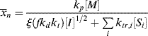
Despite the secondary effect of [I]o on the rate, it has a strong influence on the average chain length. The greater the rate of radical generation, the greater will be the frequency of alternation between chain growth and termination in a particle, resulting in a lower chain length. If rc represents the rate of radical capture/L of reaction mass (half of which produces dead chains), in the absence of chain transfer:
(9.72) 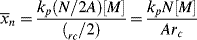
The rate of generation of radicals is based on the presence of initiator in the aqueous phase alone:
If a steady-state radical concentration is assumed,
(9.74) 
where ϕa is the volume fraction aqueous phase. Thus,
(9.75) 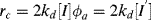
where [I′] = [I] ϕa, the moles of initiator per total volume of the reaction mass and

The chain length is, therefore, inversely proportional to the first power of initiator concentration (compare with the second-order behavior for homogeneous polymerizations in Eq. 9.27).
It must be emphasized that the preceding is a simplified view of an extremely complex process. Even within Stage II, Smith and Ewart pointed out that their case 2 was merely the middle of a spectrum. At one end of the spectrum, case 1, the average number of radicals per particle is much less than 1/2. This is believed to occur sometimes because of radical escape from the particles. At the other extreme, the average number of radicals per particle is much greater than 1/2. This comes about from large particles and/or small kt, both of which slow termination. Under these conditions, each particle acts as a tiny homogeneous reactor, according to the kinetics and the mechanism previously developed for homogeneous free-radical addition. The transition from case 2 to case 3 kinetics is often observed in seeded emulsion polymerizations, where the particles are fairly large to begin with and grow from there as the reaction proceeds.
The Smith–Ewart theory was developed for monomers such as styrene, with very low water solubility. Monomers such as acrylonitrile, with appreciable water solubility (on the order of 10%), may undergo significant homogeneous initiation in the aqueous phase. In some emulsion systems, the particles flocculate (coalesce) during polymerization, not only making a kinetic description difficult, but also sometimes badly fouling reactors. Good reviews of this subject are available [8–11], as well as complete books [7, 12–15].
9.14 Summary
Addition polymerizations are industrially important, and the basics of these reactions have been introduced in a generalized sense that is applicable to most monomers with a polymerizable double bond (including vinyl and acrylic monomers). Free-radical polymerizations proceed by a three-step mechanism (initiation, propagation, and termination). Some of the important characteristics of addition polymerization are contrasted with step-growth polymerization in Table 9.1, as well as the cartoon shown in Figure 9.1. It is difficult to have a direct comparison of the two reaction mechanisms, since some terms (such as critical gelation point) are only relevant in one case. A great resource for the kinetics of free-radical and many other types of polymerization are covered in Reference 16. In the next chapters, specialized polymerizations as well as the design of polymerization processes used in the industry are described.
Notes
1. Note that ν only includes the growing polymer chains, ignoring the monomer (X = 1) remaining in the reactor. This is different from the calculations of  in Chapter 8 for step-growth polymers, but is reflective of the length of polymers formed in free-radical polymerizations, assuming that the monomer remaining at the end of the reaction is separated from the polymer.
Problems
 according to this mechanism. Neglect chain transfer.
 , <
, < >, and their variation with conversion in an isothermal batch reactor.
 )?
)?
 just after the kick to
  just before the kick and
 (t → ∞) and <
 >(t → ∞) for this batch. You may neglect volume change.
 (70 °C)/
 (60 °C) for the emulsion polymerization:

 , <
, < >, and the polydispersity index <
 >/<
>/< > for the homogeneous, isothermal styrene polymerization of Examples 9.1. and 9.27′.
 and <
and < > on the same coordinates versus time for the period described.
 , and
, and > (t → ∞) assuming termination by disproportionation.
1. Levenspiel, O., Chemical Reaction Engineering, 2nd ed., Wiley, New York, 1972.
2. Kenat, T., R.I. Kermode, and S.L. Rosen, J. Appl. Polym. Sci. 13, 1353 (1969).
3. Hoffman, B.F., S. Schreiber, and G. Rosen, Ind. Eng. Chem. 56(5), 51 (1964).
4. Harkins, W.D., J. Am. Chem. Soc. 69, 1428 (1947).
5. Smith, W.V. and R.H. Ewart, J. Chem. Phys. 16(6), 592 (1948).
6. Flory, P.J., Principles of Polymer Chemistry, Cornell UP, Ithaca, NY, 1953, Chapter V-3.
7. Bovey, F.A., et al., Emulsion Polymerization, Interscience, New York, 1955.
8. Gardon, J.L., Emulsion polymerization, Chapter 6 in Polymerization Processes, C. E. Schildknechtand I. Skeist (eds), Wiley, New York, 1977.
9. Ugelstad, J. and F.K. Hansen, Rubber Chem. Technol. 49, 536 (1976).
10. Blackley, D.C., Macromol. Chem. (London) 2, 31 (1982).
11. Poehlein, G.W., Chapter 6 in Applied Polymer Science, 2nd ed., R.W. Tessand G. W. Poehlein (eds), ACS Symposium Series 285, American Chemical Society, Washington, DC, 1985.
12. Blackley, D.C., Emulsion Polymerization, Wiley, New York, 1975.
13. Piirma, I. and J.L. Gardon (eds), Emulsion Polymerization, ACS Symposium Series 24, American Chemical Society, Washington, DC, 1976.
14. Bassett, D.R.and A.E. Hamielec (eds), Emulsion Polymers and Emulsion Polymerization, ACS Symposium Series 165, American Chemical Society, Washington, DC, 1981.
15. Piirma, I. (ed.), Emulsion Polymerization, Academic, New York, 1982.
16. Odian, G., Principles of Polymerization, Wiley, New York, 1991.