sample size
Sampling |
CHAPTER 8 |
Sampling is a crucial element of research, and this chapter introduces key issues in sampling, including:
sample size
sampling error
sample representativeness
access to the sample
sampling strategy
probability samples
non-probability samples
sampling in qualitative research
sampling in mixed methods research
planning the sampling
The quality of a piece of research not only stands or falls by the appropriateness of methodology and instrumentation but also by the suitability of the sampling strategy that has been adopted. Questions of sampling arise directly out of the issue of defining the population on which the research will focus.
Researchers must take sampling decisions early in the overall planning of a piece of research. Factors such as expense, time and accessibility frequently prevent researchers from gaining information from the whole population. Therefore they often need to be able to obtain data from a smaller group or subset of the total population in such a way that the knowledge gained is representative of the total population (however defined) under study. This smaller group or subset is the sample. Experienced researchers start with the total population and work down to the sample. By contrast, less experienced researchers often work from the bottom up, that is, they determine the minimum number of respondents needed to conduct the research (Bailey, 1994). However, unless they identify the total population in advance, it is virtually impossible for them to assess how representative the sample is that they have drawn.
Suppose that a class teacher has been released from her teaching commitments for one month in order to conduct some research into the abilities of 13-year-old students to undertake a set of science experiments; that the research is to draw on three secondary schools which contain 300 such students each, a total of 900 students, and that the method that the teacher has been asked to use for data collection is a semi-structured interview. Because of the time available to the teacher it would be impossible for her to interview all 900 students (the total population being all the cases). Therefore she has to be selective and to interview fewer than all 900 students. How will she decide that selection; how will she select which students to interview?
If she were to interview 200 of the students, would that be too many? If she were to interview just 20 of the students would that be too few? If she were to interview just the males or just the females, would that give her a fair picture? If she were to interview just those students whom the science teachers had decided were ‘good at science’, would that yield a true picture of the total population of 900 students? Perhaps it would be better for her to interview those students who were experiencing difficulty in science and who did not enjoy science, as well as those who were ‘good at science’. Suppose that she turns up on the days of the interviews only to find that those students who do not enjoy science have decided to absent themselves from the science lesson. How can she reach those students?
Decisions and problems such as these face researchers in deciding the sampling strategy to be used. Judgements have to be made about five key factors in sampling:
1 the sample size;
2 the representativeness and parameters of the sample;
3 access to the sample;
4 the sampling strategy to be used;
5 the kind of research that is being undertaken (e.g. quantitative/qualitative/mixed methods).
The decisions here will determine the sampling strategy to be used. This assumes that a sample is actually required; there may be occasions on which the researcher can access the whole population rather than a sample.
A question that often plagues novice researchers is just how large their samples for the research should be. There is no clear-cut answer, for the correct sample size depends on the purpose of the study, the nature of the population under scrutiny, the level of accuracy required, the anticipated response rate, the number of variables that are included in the research, and whether the research is quantitative or qualitative. However, it is possible to give some advice on this matter. Generally speaking, for quantitative research, the larger the sample the better, as this not only gives greater reliability but also enables more sophisticated statistics to be used.
Thus, a sample size of 30 is held by many to be the minimum number of cases if researchers plan to use some form of statistical analysis on their data, though this is a very small number and we would advise very considerably more. Researchers need to think out in advance of any data collection the sorts of relationships that they wish to explore within subgroups of their eventual sample. The number of variables researchers set out to control in their analysis and the types of statistical tests that they wish to make must inform their decisions about sample size prior to the actual research undertaking. Typically an anticipated minimum of 30 cases per variable should be used as a ‘rule of thumb’, i.e. one must be assured of having a minimum of 30 cases for each variable (of course, the 30 cases for variable one could also be the same 30 as for variable two), though this is a very low estimate indeed. This number rises rapidly if different subgroups of the population are included in the sample (discussed below), which is frequently the case.
Further, depending on the kind of analysis to be performed, some statistical tests will require larger samples. For example, let us imagine that one wished to calculate the chi-square statistic, a commonly used test (discussed in Part 5) with crosstabulated data, for example looking at two subgroups of stakeholders in a primary school containing 60 10 year olds and 20 teachers and their responses to a question on a five-point scale.
Here one can notice that the sample size is 80 cases, an apparently reasonably sized sample. However, six of the ten cells of responses (60 per cent) contain fewer than five cases. The chi-square statistic requires there to be five cases or more in 80 per cent of the cells (i.e. eight out of the ten cells). In this example only 40 per cent of the cells contained more than five cases, so even with a comparatively large sample, the statistical requirements for reliable data with a straightforward statistic such as chi-square have not been met. The message is clear, one needs to anticipate, as far as one is able, some possible distributions of the data and see if these will prevent appropriate statistical analysis; if the distributions look unlikely to enable reliable statistics to be calculated then one should increase the sample size, or exercise great caution in interpreting the data because of problems of reliability, or not use particular statistics, or, indeed, consider abandoning the exercise if the increase in sample size cannot be achieved.
Variable: 10 year olds should do one hour’s homework each weekday evening | |||||
|
Strongly disagree |
Disagree |
Neither agree nor disagree |
Agree |
Strongly agree |
10-year-old pupils in the school |
25 |
20 |
3 |
8 |
4 |
Teachers in the school |
6 |
4 |
2 |
4 |
4 |
The point here is that each variable may need to be ensured of a reasonably large sample size (a minimum of maybe six to ten cases). Indeed Gorard (2003: 63) suggests that one can start from the minimum number of cases required in each cell, multiply this by the number of cells, and then double the total. In the example above, with six cases in each cell, the minimum sample would be 120 (6 × 10 × 2), though, to be on the safe side, to try to ensure ten cases in each cell, a minimum sample of 200 might be better (10 × 10 × 2), though even this is no guarantee.
The issue arising out of the example here is also that one can observe considerable variation in the responses from the participants in the research. Gorard (2003: 62) suggests that if a phenomenon contains a lot of potential variability then this will increase the sample size. Surveying a variable such as IQ (intelligence quotient) for example, with a potential range from 70 to around 150, may require a larger sample rather than a smaller sample.
As well as the requirement of a minimum number of cases in order to examine relationships between subgroups, researchers must obtain the minimum sample size that will accurately represent the population being targeted. With respect to size, will a large sample guarantee representativeness? Not necessarily! In our first example of the class teacher’s research, she could have interviewed a total sample of 450 females and still not have represented the male population. Will a small size guarantee representativeness? Again, not necessarily! The latter could fall into the trap of saying that 50 per cent of those who expressed an opinion said that they enjoyed science, when the 50 per cent was only one student, a researcher having interviewed only two students in all. Furthermore, too large a sample might become unwieldy and too small a sample might be unrepresentative (e.g. in the first example, the researcher might have wished to interview 450 students but this would have been unworkable in practice or the researcher might have interviewed only ten students, which, in all likelihood, would have been unrepresentative of the total population of 900 students).
Where simple random sampling is used, the sample size needed to reflect the population value of a particular variable depends both on the size of the population and the amount of heterogeneity in the population (Bailey, 1994). Generally, for populations of equal heterogeneity, the larger the population, the larger the sample that must be drawn. For populations of equal size, the greater the heterogeneity on a particular variable, the larger the sample that is needed. To the extent that a sample fails to represent accurately the population involved, there is sampling error, discussed below.
Sample size is also determined to some extent by the style of the research. For example, a survey style usually requires a large sample, particularly if inferential statistics are to be calculated. In ethnographic or qualitative research it is more likely that the sample size will be small. Sample size might also be constrained by cost – in terms of time, money, stress, administrative support, the number of researchers and resources. Borg and Gall (1979: 194–5) suggest that correlational research requires a sample size of no fewer than 30 cases, that causal-comparative and experimental methodologies require a sample size of no fewer than 15 cases, and that survey research should have no fewer than 100 cases in each major subgroup and 20 to 50 in each minor subgroup.
They advise (Borg and Gall, 1979: 186) that sample size has to begin with an estimation of the smallest number of cases in the smallest subgroup of the sample, and ‘work up’ from that, rather than vice versa. So, for example, if 5 per cent of the sample must be teenage boys, and this subsample must be 30 cases (e.g. for correlational research), then the total sample will be 30 ÷ 0.05 = 600; if 15 per cent of the sample must be teenage girls and the subsample must be 45 cases, then the total sample must be 45 ÷ 0.15 = 300 cases.
The size of a probability (random) sample can be determined in two ways, either by the researcher exercising prudence and ensuring that the sample represents the wider features of the population with the minimum number of cases or by using a table which, from a mathematical formula, indicates the appropriate size of a random sample for a given number of the wider population (Morrison, 1993: 117). One such example is provided by Krejcie and Morgan (1970), whose work suggests that if the researcher were devising a sample from a wider population of 30 or fewer (e.g. a class of students or a group of young children in a class) then she/he would be well advised to include the whole of the wider population as the sample.
Krejcie and Morgan (1970) indicate that the smaller the number of cases there are in the wider, whole population, the larger the proportion of that population must be which appears in the sample; the converse of this is true: the larger the number of cases there are in the wider, whole population, the smaller the proportion of that population can be which appears in the sample. They note that as the population increases the proportion of the population required in the sample diminishes and, indeed, remains constant at around 384 cases (p. 610). Hence, for example, a piece of research involving all the children in a small primary or elementary school (up to 100 students in all) might require between 80 per cent and 100 per cent of the school to be included in the sample, whilst a large secondary school of 1,200 students might require a sample of 25 per cent of the school in order to achieve randomness. As a rough guide in a random sample, the larger the sample, the greater is its chance of being representative.
In determining sample size for a probability sample one has to consider not only the population size but also the error margins that one wishes to tolerate. These are expressed in terms of the confidence level and confidence interval, two further pieces of terminology. The confidence level, usually expressed as a percentage (usually 95 per cent or 99 per cent), is an index of how sure we can be (95 per cent of the time or 99 per cent of the time) that the responses lie within a given variation range. The confidence interval is that degree of variation or variation range (e.g. ± 1 per cent, or ± 2 per cent, or ± 3 per cent) that one wishes to ensure. For example the confidence interval in many opinion polls is ± 3 per cent; this means that, if a voting survey indicates that a political party has 52 per cent of the votes then it could be as low as 49 per cent (52 – 3) or as high as 55 per cent (52 + 3). A confidence level of 95 per cent here would indicate that we could be sure of this result within this range (± 3 per cent) for 95 per cent of the time.
If we want to have a very high confidence level (say 99 per cent of the time) then the sample size will be high. On the other hand, if we want a less stringent confidence level (say 90 per cent of the time), then the sample size will be smaller. Usually a compromise is reached, and researchers opt for a 95 per cent confidence level. Similarly, if we want a very small confidence interval (i.e. a limited range of variation, e.g. 3 per cent) then the sample size will be high, and if we are comfortable with a larger degree of variation (e.g. 5 per cent) then the sample size will be lower.
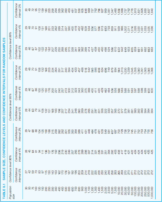
A full table of sample sizes for a probability sample is given in Table 8.1, with three confidence levels (90 per cent, 95 per cent and 99 per cent) and three confidence intervals (5 per cent, 4 per cent and 3 per cent). We can see that the size of the sample reduces at an increasing rate as the population size increases; generally (but, clearly, not always) the larger the population, the smaller the proportion the probability sample can be. Also, the higher the confidence level, the greater the sample, and the lower the confidence interval, the higher the sample. A conventional sampling strategy will be to use a 95 per cent confidence level and a 3 per cent confidence interval.
There are several websites that offer sample size calculation services for random samples. Some free sites at the time of writing are:
www.surveysystem.com/sscalc.htm;
www.macorr.com/ss_calculator.htm;
www.raosoft.com/samplesize.html;
www.researchinfo.com/docs/calculators/samplesize.cfm;.
www.nss.gov.au/nss/home.nsf/pages/Sample+Size+Calculator+Description?OpenDocument.
Here the researcher inputs the desired confidence level, confidence interval, and the population size, and the sample size is automatically calculated.
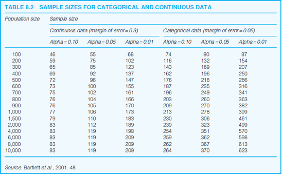
A further consideration in the determination of sample size is the nature of the variables included. Bartlett et al. (2001) indicate that sample sizes for categorical variables (e.g. sex, education level) will differ from those of continuous data (e.g. marks in a test, money in the bank); they show that typically categorical data require larger samples than continuous data. They provide a summary table (Table 8.2) to indicate the different sample sizes required for categorical and continuous data:
Within the discussion of categorical and continuous variables, Bartlett et al. (2001: 45) suggest that, for categorical data a 5 per cent margin of error is commonplace, whilst for continuous data, a 3 per cent margin of error is usual, and these are the intervals that they use in their table (Table 8.2). One can see that, for both categorical and continuous data, the proportion of the population decreases as the sample increases, and that, for continuous data, there is no difference in the sample sizes for populations of 2,000 or more. The researcher should normally opt for the larger sample size (i.e. the sample size required for categorical data) if both categorical and continuous data are being used.
Bartlett et al. (2001: 48–9) also suggest that the sample size will vary according to the statistics that will be required to be used. They suggest that if multiple regressions are to be calculated then ‘the ratio of observations [cases] to independent variables should not fall below five’, though some statisticians suggest a ratio of 10 to 1, particularly for continuous data, as, in continuous data, the sample sizes tend to be smaller than for categorical data. They also suggest that, in multiple regression: (a) for continuous data, if the number of independent variables is in the ratio of 5 to 1 then the sample size should be no fewer than 111 and the number of regressors (independent variables) should be no more than 22; (b) for continuous data, if the number of independent variables is in the ratio of 10 to 1 then the sample size should be no fewer than 111 and the number of regressors (independent variables) should be no more than 11; (c) for categorical data, if the number of independent variables is in the ratio of 5 to 1 then the sample size should be no fewer than 313 and the number of regressors (independent variables) should be no more than 62; (d) for categorical data, if the number of independent variables is in the ratio of 10 to 1 then the sample size should be no fewer than 313 and the number of regressors (independent variables) should be no more than 31. Bartlett et al. (2001: 49) also suggest that, for factor analysis, a sample size of no fewer than 100 observations (cases) should be the general rule.
If different subgroups or strata (discussed below) are to be used then the requirements placed on the total sample also apply to each subgroup. For example, let us imagine that we are surveying a whole school of 1,000 students in a multi-ethnic school. The formulae above suggest that we need 278 students in our random sample, to ensure representativeness. However, let us imagine that we wished to stratify our groups into, for example, Chinese (100 students), Spanish (50 students), English (800 students) and American (50 students). From tables of random sample sizes we work out a random sample:
|
Population |
Sample |
Chinese |
100 |
80 |
Spanish |
50 |
44 |
English |
800 |
260 |
American |
50 |
44 |
Total |
1,000 |
428 |
Our original sample size of 278 has now increased, very quickly, to 428. The message is very clear: the greater the number of strata (subgroups), the larger the sample will be. Much educational research concerns itself with strata rather than whole samples, so the issue is significant. One can rapidly generate the need for a very large sample. If subgroups are required then the same rules for calculating overall sample size apply to each of the subgroups.
Further, determining the size of the sample will also have to take account of non-response, attrition and respondent mortality, i.e. some participants will fail to return questionnaires, leave the research, return incomplete or spoiled questionnaires (e.g. missing out items, putting two ticks in a row of choices instead of only one). Hence it is advisable to overestimate (oversample) rather than to underestimate the size of the sample required, to build in redundancy (Gorard, 2003: 60). Unless one has guarantees of access, response and, perhaps, the researcher’s own presence at the time of conducting the research (e.g. presence when questionnaires are being completed), then it might be advisable to estimate up to double the size of the required sample in order to allow for such loss of clean and complete copies of questionnaires/responses.
Further, with very small subgroups of populations, it may be necessary to operate a weighted sample – an oversampling – in order to gain any responses at all as, if a regular sample were to be gathered, there would be so few people included as to risk being unrepresentative of the subgroup in question. A weighted sample, in this instance, is where a higher proportion of the subgroup is sampled, and then the results are subsequently scaled down to be fairer in relation to the whole sample.
In some circumstances, meeting the requirements of sample size can be done on an evolutionary basis. For example, let us imagine that you wish to sample 300 teachers, randomly selected. You succeed in gaining positive responses from 250 teachers to, for example, a telephone survey or a questionnaire survey, but you are 50 short of the required number. The matter can be resolved simply by adding another 50 to the random sample, and, if not all of these are successful, then adding some more until the required number is reached.
Borg and Gall (1979: 195) suggest that, as a general rule, sample sizes should be large where:
there are many variables;
only small differences or small relationships are expected or predicted;
the sample will be broken down into subgroups;
the sample is heterogeneous in terms of the variables under study;
reliable measures of the dependent variable are unavailable.
Oppenheim (1992: 44) adds to this the view that the nature of the scales to be used also exerts an influence on the sample size. For nominal data the sample sizes may well have to be larger than for interval and ratio data (i.e. a variant of the issue of the number of subgroups to be addressed, the greater the number of subgroups or possible categories, the larger the sample will have to be).
Borg and Gall (1979) set out a formula-driven approach to determining sample size (see also Moser and Kalton, 1977; Ross and Rust, 1997: 427–38), and they also suggest using correlational tables for correlational studies – available in most texts on statistics – as it were ‘in reverse’ to determine sample size (p. 201), i.e. looking at the significance levels of correlation coefficients and then reading off the sample sizes usually required to demonstrate that level of significance. For example, a correlational significance level of 0.01 would require a sample size of ten if the estimated coefficient of correlation is 0.65, or a sample size of 20 if the estimated correlation coefficient is 0.45, and a sample size of 100 if the estimated correlation co-efficient is 0.20. Again, an inverse proportion can be seen – the larger the sample population, the smaller the estimated correlation co-efficient can be to be deemed significant.
With both qualitative and quantitative data, the essential requirement is that the sample is representative of the population from which it is drawn. In a dissertation concerned with a life history (i.e. n = 1), the sample is the population!
In a qualitative study of 30 highly able girls of similar socio-economic background following an A-level Biology course, a sample of five or six may suffice the researcher who is prepared to obtain additional corroborative data by way of validation.
Where there is heterogeneity in the population, then a larger sample must be selected on some basis that respects that heterogeneity. Thus, from a staff of 60 secondary school teachers differentiated by gender, age, subject specialism, management or classroom responsibility, etc., it would be insufficient to construct a sample consisting of ten female classroom teachers of Arts and Humanities subjects.
For quantitative data, a precise sample number can be calculated according to the level of accuracy and the level of probability that the researcher requires in her work. She can then report in her study the rationale and the basis of her research decision (Blalock, 1979).
By way of example, suppose a teacher/researcher wishes to sample opinions among 1,000 secondary school students. She intends to use a 10-point scale ranging from 1 = totally unsatisfactory to 10 = absolutely fabulous. She already has data from her own class of 30 students and suspects that the responses of other students will be broadly similar. Her own students rated the activity (an extra-curricular event) as follows: mean score = 7.27; standard deviation = 1.98. In other words, her students were pretty much ‘bunched’ about a warm, positive appraisal on the 10-point scale. How many of the 1,000 students does she need to sample in order to gain an accurate (i.e. reliable) assessment of what the whole school (n = 1,000) thinks of the extracurricular event? It all depends on what degree of accuracy and what level of probability she is willing to accept.
A simple calculation from a formula by Blalock (1979: 215–18) shows that:
if she is happy to be within + or – 0.5 of a scale point and accurate 19 times out of 20, then she requires a sample of 60 out of the 1,000;
if she is happy to be within + or – 0.5 of a scale point and accurate 99 times out of 100, then she requires a sample of 104 out of the 1,000;
if she is happy to be within + or – 0.5 of a scale point and accurate 999 times out of 1,000, then she requires a sample of 170 out of the 1,000;
if she is a perfectionist and wishes to be within + or – 0.25 of a scale point and accurate 999 times out of 1,000, then she requires a sample of 679 out of the 1,000.
It is clear that sample size is a matter of judgement as well as mathematical precision; even formula-driven approaches make it clear that there are elements of prediction, standard error and human judgement involved in determining sample size.
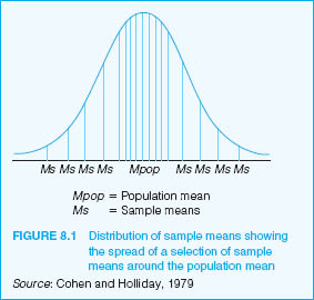
If many samples are taken from the same population, it is unlikely that they will all have characteristics identical with each other or with the population; their means will be different. In brief, there will be sampling error (see Cohen and Holliday, 1979, 1996). Sampling error is often taken to be the difference between the sample mean and the population mean. Sampling error is not necessarily the result of mistakes made in sampling procedures. Rather, variations may occur due to the chance selection of different individuals. For example, if we take a large number of samples from the population and measure the mean value of each sample, then the sample means will not be identical. Some will be relatively high, some relatively low, and many will cluster around an average or mean value of the samples. We show this diagrammatically in Figure 8.1.
Why should this occur? We can explain the phenomenon by reference to the Central Limit Theorem which is derived from the laws of probability. This states that if random large samples of equal size are repeatedly drawn from any population, then the mean of those samples will be approximately normally distributed. The distribution of sample means approaches the normal distribution as the size of the sample increases, regardless of the shape – normal or otherwise – of the parent population (Hopkins et al., 1996: 159, 388). Moreover, the average or mean of the sample means will be approximately the same as the population mean. Hopkins et al. (1996: 159–62) demonstrate this by reporting the use of computer simulation to examine the sampling distribution of means when computed 10,000 times (a method that we discuss in Chapter 10). Rose and Sullivan (1993: 144) remind us that 95 per cent of all sample means fall between plus or minus 1.96 standard errors of the sample and population means, i.e. that we have a 95 per cent chance of having a single sample mean within these limits, that the sample mean will fall within the limits of the population mean.
By drawing a large number of samples of equal size from a population, we create a sampling distribution. We can calculate the error involved in such sampling. The standard deviation of the theoretical distribution of sample means is a measure of sampling error and is called the standard error of the mean (SEM). Thus,

where SDS = the standard deviation of the sample and N = the number in the sample.
Strictly speaking, the formula for the standard error of the mean is:

where SDpop = the standard deviation of the population.
However, as we are usually unable to ascertain the SD of the total population, the standard deviation of the sample is used instead. The standard error of the mean provides the best estimate of the sampling error. Clearly, the sampling error depends on the variability (i.e. the heterogeneity) in the population as measured by SDpop as well as the sample size (N ) (Rose and Sullivan, 1993: 143). The smaller the SDpop the smaller the sampling error; the larger the N, the smaller the sampling error. Where the SDpop is very large, then N needs to be very large to counteract it. Where SDpop is very small, then N, too, can be small and still give a reasonably small sampling error. As the sample size increases the sampling error decreases. Hopkins et al. (1996: 159) suggest that, unless there are some very unusual distributions, samples of 25 or greater usually yield a normal sampling distribution of the mean. For further analysis of steps that can be taken to cope with the estimation of sampling in surveys we refer the reader to Ross and Wilson (1997).
We said earlier that one answer to ‘How big a sample must I obtain?’ is ‘How accurate do I want my results to be?’ This is well illustrated in the following example: a school principal finds that the 25 students she talks to at random are reasonably in favour of a proposed change in the lunch break hours, 66 per cent being in favour and 34 per cent being against. How can she be sure that these proportions are truly representative of the whole school of 1,000 students?
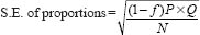
A simple calculation of the standard error of proportions provides the principal with her answer.

where
P = the percentage in favour
Q = 100 per cent – P
N = the sample size.
The formula assumes that each sample is drawn on a simple random basis. A small correction factor called the finite population correction (fpc) is generally applied as follows:
where f is the proportion included in the sample.
Where, for example, a sample is 100 out of 1,000, f is 0.1.
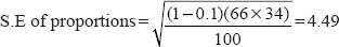
With a sample of 25, the S.E. = 9.4. In other words, the favourable vote can vary between 56.6 per cent and 75.4 per cent; likewise, the unfavourable vote can vary between 43.4 per cent and 24.6 per cent. Clearly, a voting possibility ranging from 56.6 per cent in favour to 43.4 per cent against is less decisive than 66 per cent as opposed to 34 per cent. Should the school principal enlarge her sample to include 100 students, then the S.E. becomes 4.5 and the variation in the range is reduced to 61.5 per cent – 70.5 per cent in favour and 38.5 per cent – 29.5 per cent against. Sampling the whole school’s opinion (n = 1,000) reduces the S.E. to 1.5 and the ranges to 64.5 per cent – 67.5 per cent in favour and 35.5 per cent – 32.5 per cent against. It is easy to see why political opinion surveys are often based upon sample sizes of 1,000 to 1,500 (Gardner, 1978).
What is being suggested here generally is that, in order to overcome problems of sampling error, in order to ensure that one can separate random effects and variation from non-random effects, and in order for the power of a statistic to be felt, one should opt for as large a sample as possible. As Gorard (2003: 62) says: ‘power is an estimate of the ability of the test you are using to separate the effect size from random variation’, and a large sample helps the researcher to achieve statistical power. Samples of fewer than 30 are dangerously small, as they allow the possibility of considerable standard error, and, for over around 80 cases, any increases to the sample size have little effect on the standard error.
The researcher will need to consider the extent to which it is important that the sample in fact represents the whole population in question (in the example above, the 1,000 students), if it is to be a valid sample. The researcher will need to be clear what it is that is being represented, i.e. to set the parameter characteristics of the wider population – the sampling frame – clearly and correctly. There is a popular example of how poor sampling may be unrepresentative and unhelpful for a researcher. A national newspaper reports that one person in every two suffers from backache; this headline stirs alarm in every doctor’s surgery throughout the land. However, the newspaper fails to make clear the parameters of the study which gave rise to the headline. It turns out that the research took place (a) in a damp part of the country where the incidence of backache might be expected to be higher than elsewhere, (b) in a part of the country which contained a disproportionate number of elderly people, again who might be expected to have more backaches than a younger population, (c) in an area of heavy industry where the working population might be expected to have more backache than in an area of lighter industry or service industries, (d) by using two doctors’ records only, overlooking the fact that many backache sufferers went to those doctors’ surgeries because the two doctors concerned were known to be overly sympathetic to backache sufferers rather than responsibly suspicious.
These four variables – climate, age group, occupation and reported incidence – were seen to exert a disproportionate effect on the study, i.e. if the study were to have been carried out in an area where the climate, age group, occupation and reporting were to have been different, then the results might have been different. The newspaper report sensationally generalized beyond the parameters of the data, thereby overlooking the limited representativeness of the study.
It is important to consider adjusting the weightings of subgroups in the sample once the data have been collected. For example, in a secondary school where half the students are male and half are female, consider the following table of pupils’ responses to the question ‘How far does your liking of the form teacher affect your attitude to school work?’:
Variable: How far does your liking of the form teacher affect your attitude to school work? | |||||
Very little |
A little |
Somewhat |
Quite a lot |
A very great deal | |
Male |
10 |
20 |
30 |
25 |
15 |
Female |
50 |
80 |
30 |
25 |
15 |
Total |
60 |
100 |
60 |
50 |
30 |
Let us say that we are interested in the attitudes according to the gender of the respondents, as well as overall. In this example one could surmise that generally the results indicate that the liking of the form teacher has only a small to moderate effect on the students’ attitude to work. However, we have to observe that twice as many girls as boys are included in the sample, and this is an unfair representation of the population of the school, which comprises 50 per cent girls and 50 per cent boys, i.e. girls are over-represented and boys are under-represented. If one equalizes the two sets of scores by gender to be closer to the school population (either by doubling the number of boys or halving the number of girls) then the results look very different, e.g.:
Variable: How far does your liking of the form teacher affect your attitude to school work? | |||||
|
Very little |
A little |
Somewhat |
Quite a lot |
A very great deal |
Male |
20 |
40 |
60 |
50 |
30 |
Female |
50 |
80 |
30 |
25 |
15 |
Total |
70 |
120 |
90 |
75 |
45 |
In this latter case a much more positive picture is painted, indicating that the students regard their liking of the form teacher as a quite important feature in their attitude to school work. Here equalizing the sample to represent more fairly the population by weighting yields a different picture. Weighting the results is an important consideration.
Access is a key issue and is an early factor that must be decided in research. Researchers will need to ensure not only that access is permitted but is, in fact, practicable. For example, if a researcher were to conduct research into truancy and unauthorized absence from school, and she decided to interview a sample of truants, the research might never commence as the truants, by definition, would not be present! Similarly access to sensitive areas might not only be difficult but problematical both legally and administratively, for example, access to child abuse victims, child abusers, disaffected students, drug addicts, school refusers, bullies and victims of bullying. In some sensitive areas access to a sample might be denied by the potential sample participants themselves, for example an AIDS counsellor might be so seriously distressed by her work that she simply cannot face discussing with a researcher the subject matter of her traumatic work; it is distressing enough to do the job without living through it again with a researcher.
Access might also be denied by the potential sample participants themselves for very practical reasons, for example a doctor or a teacher simply might not have the time to spend with the researcher. Further, access might be denied by people who have something to protect, for example a school which has recently received a very poor inspection result or poor results on external examinations, or a person who has made an important discovery or a new invention and who does not wish to disclose the secret of her success; the trade in intellectual property has rendered this a live issue for many researchers. There are very many reasons which might prevent access to the sample, and researchers cannot afford to neglect this potential source of difficulty in planning research.
In many cases access is guarded by ‘gatekeepers’ – people who can control the researcher’s access to those whom she/he really wants to target. For school staff this might be, for example, headteachers, school governors, school secretaries, form teachers; for pupils this might be friends, gang members, parents, social workers and so on. It is critical for researchers not only to consider whether access is possible but how access will be undertaken – to whom does one have to go, both formally and informally, to gain access to the target group.
Not only might access be difficult but its corollary – release of information – might be problematic. For example, a researcher might gain access to a wealth of sensitive information and appropriate people, but there might be a restriction on the release of the data collection; in the field of education in the UK reports have been known to be suppressed, delayed or ‘doctored’. It is not always enough to be able to ‘get to’ the sample, the problem might be to ‘get the information out’ to the wider public, particularly if it could be critical of powerful people.
There are two main methods of sampling (Cohen and Holliday, 1979, 1982, 1996; Schofield, 1996). The researcher must decide whether to opt for a probability (also known as a random sample) or a non-probability sample (also known as a purposive sample). The difference between them is this: in a probability sample the chances of members of the wider population being selected for the sample are known, whereas in a non-probability sample the chances of members of the wider population being selected for the sample are unknown. In the former (probability sample) every member of the wider population has an equal chance of being included in the sample; inclusion or exclusion from the sample is a matter of chance and nothing else. In the latter (non-probability sample) some members of the wider population definitely will be excluded and others definitely included (i.e. every member of the wider population does not have an equal chance of being included in the sample). In this latter type the researcher has deliberately – purposely – selected a particular section of the wider population to include in or exclude from the sample.
A probability sample, because it draws randomly from the wider population, will be useful if the researcher wishes to be able to make generalizations, because it seeks representativeness of the wider population. (It also permits two-tailed tests to be administered in statistical analysis of quantitative data.) This is a form of sampling that is popular in randomized controlled trials. On the other hand, a non-probability sample deliberately avoids representing the wider population; it seeks only to represent a particular group, a particular named section of the wider population, e.g. a class of students, a group of students who are taking a particular examination, a group of teachers.
A probability sample will have less risk of bias than a non-probability sample, whereas, by contrast, a non-probability sample, being unrepresentative of the whole population, may demonstrate skewness or bias. (For this type of sample a one-tailed test will be used in processing statistical data.) This is not to say that the former is bias-free; there is still likely to be sampling error in a probability sample (discussed below), a feature that has to be acknowledged; for example opinion polls usually declare their error factors, e.g. ± 3 per cent.
There are several types of probability samples: simple random samples; systematic samples; stratified samples; cluster samples; stage samples; and multiphase samples. They all have a measure of randomness built into them and therefore have a degree of generalizability.
In simple random sampling, each member of the population under study has an equal chance of being selected and the probability of a member of the population being selected is unaffected by the selection of other members of the population, i.e. each selection is entirely independent of the next. The method involves selecting at random from a list of the population (a sampling frame) the required number of subjects for the sample. This can be done by drawing names out of a hat until the required number is reached, or by using a table of random numbers set out in matrix form (these are reproduced in many books on quantitative research methods and statistics), and allocating these random numbers to participants or cases (e.g. Hopkins et al., 1996: 148–9). Because of probability and chance, the sample should contain subjects with characteristics similar to the population as a whole; some old, some young, some tall, some short, some fit, some unfit, some rich, some poor, etc. One problem associated with this particular sampling method is that a complete list of the population is needed and this is not always readily available.
This method is a modified form of simple random sampling. It involves selecting subjects from a population list in a systematic rather than a random fashion. For example, if from a population of, say, 2,000, a sample of 100 is required, then every twentieth person can be selected. The starting point for the selection is chosen at random.
One can decide how frequently to make systematic sampling by a simple statistic – the total number of the wider population being represented divided by the sample size required:

f = frequency interval
N = the total number of the wider population
sn = the required number in the sample.
Let us say that the researcher is working with a school of 1,400 students; by looking at the table of sample size (Table 8.1) required for a random sample of these 1,400 students we see that 301 students are required to be in the sample. Hence the frequency interval (f ) is:
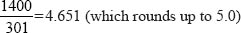
Hence the researcher would pick out every fifth name on the list of cases.
Such a process, of course, assumes that the names on the list themselves have been listed in a random order. A list of females and males might list all the females first, before listing all the males; if there were 200 females on the list, the researcher might have reached the desired sample size before reaching that stage of the list which contained males, thereby distorting (skewing) the sample. Another example might be where the researcher decides to select every thirtieth person identified from a list of school students, but it happens that: (a) the school has just over 30 students in each class; (b) each class is listed from high ability to low ability students; (c) the school listing identifies the students by class.
In this case, although the sample is drawn from each class, it is not fairly representing the whole school population since it is drawing almost exclusively on the lower ability students. This is the issue of periodicity (Calder, 1979). Not only is there the question of the order in which names are listed in systematic sampling, but there is also the issue that this process may violate one of the fundamental premises of probability sampling, namely that every person has an equal chance of being included in the sample. In the example above where every fifth name is selected, this guarantees that names 1–4, 6–9, etc. will be excluded, i.e. everybody does not have an equal chance to be chosen. The ways to minimize this problem are to ensure that the initial listing is selected randomly and that the starting point for systematic sampling is similarly selected randomly.
Random stratified sampling involves dividing the population into homogenous groups, each group containing subjects with similar characteristics. For example, group A might contain males and group B, females. In order to obtain a sample representative of the whole population in terms of sex, a random selection of subjects from group A and group B must be taken. If needed, the exact proportion of males to females in the whole population can be reflected in the sample. The researcher will have to identify those characteristics of the wider population which must be included in the sample, i.e. to identify the parameters of the wider population. This is the essence of establishing the sampling frame.
To organize a stratified random sample is a simple two-stage process. First, identify those characteristics which appear in the wider population which must also appear in the sample, i.e. divide the wider population into homogenous and, if possible, discrete groups (strata), for example males and females. Second, randomly sample within these groups, the size of each group being determined either by the judgement of the researcher or by reference to Tables 8.1 or 8.2.
The decision on which characteristics to include should strive for simplicity as far as possible, as the more factors there are, not only the more complicated the sampling becomes, but often the larger the sample will have to be to include representatives of all strata of the wider population.
A random stratified sample is, therefore, a useful blend of randomization and categorization, thereby enabling both a quantitative and qualitative piece of research to be undertaken. A quantitative piece of research will be able to use analytical and inferential statistics, whilst a qualitative piece of research will be able to target those groups in institutions or clusters of participants who will be able to be approached to participate in the research.
When the population is large and widely dispersed, gathering a simple random sample poses administrative problems. Suppose we want to survey students’ fitness levels in a particularly large community or across a country. It would be completely impractical to select students randomly and spend an inordinate amount of time travelling about in order to test them. By cluster sampling, the researcher can select a specific number of schools and test all the students in those selected schools, i.e. a geographically close cluster is sampled.
One would have to be careful to ensure that cluster sampling does not build in bias. For example, let us imagine that we take a cluster sample of a city in an area of heavy industry or great poverty; this may not represent all kinds of cities or socio-economic groups, i.e. there may be similarities within the sample that do not catch the variability of the wider population. The issue here is one of representativeness; hence it might be safer to take several clusters and to sample lightly within each cluster, rather to take fewer clusters and sample heavily within each.
Cluster samples are widely used in small-scale research. In a cluster sample the parameters of the wider population are often drawn very sharply; a researcher, therefore, would have to comment on the generalizability of the findings. The researcher may also need to stratify within this cluster sample if useful data, i.e. those which are focused and which demonstrate discriminability, are to be acquired.
Stage sampling is an extension of cluster sampling. It involves selecting the sample in stages, that is, taking samples from samples. Using the large community example in cluster sampling, one type of stage sampling might be to select a number of schools at random, and from within each of these schools, select a number of classes at random, and from within those classes select a number of students.
Morrison (1993: 121–2) provides an example of how to address stage sampling in practice. Let us say that a researcher wants to administer a questionnaire to all 16 year olds in each of 11 secondary schools in one region. By contacting the 11 schools she finds that there are 2,000 16 year olds on roll. Because of questions of confidentiality she is unable to find out the names of all the students so it is impossible to draw their names out of a hat to achieve randomness (and even if she had the names, it would be a mind-numbing activity to write out 2,000 names to draw out of a hat!). From looking at Table 8.1 she finds that, for a random sample of the 2,000 students, the sample size is 322 students. How can she proceed?
The first stage is to list the 11 schools on a piece of paper and then to put the names of the 11 schools onto a small card and place each card in a hat. She draws out the first name of the school, puts a tally mark by the appropriate school on her list and returns the card to the hat. The process is repeated 321 times, bringing the total to 322. The final totals might appear thus:
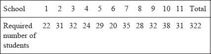
For the second stage she then approaches the 11 schools and asks each of them to select randomly the required number of students for each school. Randomness has been maintained in two stages and a large number (2,000) has been rendered manageable. The process at work here is to go from the general to the specific, the wide to the focused, the large to the small. Caution has to be exercised here, as the assumption is that the schools are of the same size and are large; that may not be the case in practice, in which case this strategy may be inadvisable.
In stage sampling there is a single unifying purpose throughout the sampling. In the previous example the purpose was to reach a particular group of students from a particular region. In a multi-phase sample the purposes change at each phase, for example, at phase one the selection of the sample might be based on the criterion of geography (e.g. students living in a particular region); phase two might be based on an economic criterion (e.g. schools whose budgets are administered in markedly different ways); phase three might be based on a political criterion (e.g. schools whose students are drawn from areas with a tradition of support for a particular political party), and so on. What is evident here is that the sample population will change at each phase of the research.
The selectivity which is built into a non-probability sample derives from the researcher targeting a particular group, in the full knowledge that it does not represent the wider population; it simply represents itself. This is frequently the case in small-scale research, for example, as with one or two schools, two or three groups of students, or a particular group of teachers, where no attempt to generalize is desired; this is frequently the case for some ethnographic research, action research or case study research. Small-scale research often uses non-probability samples because, despite the disadvantages that arise from their non-representativeness, they are far less complicated to set up, are considerably less expensive and can prove perfectly adequate where researchers do not intend to generalize their findings beyond the sample in question, or where they are simply piloting a questionnaire as a prelude to the main study.
Just as there are several types of probability sample, so there are several types of non-probability sample: convenience sampling, quota sampling, purposive sampling, dimensional sampling and snowball sampling. Each type of sample seeks only to represent itself or instances of itself in a similar population, rather than attempting to represent the whole, undifferentiated population.
Convenience sampling – or, as it is sometimes called, accidental or opportunity sampling – involves choosing the nearest individuals to serve as respondents and continuing that process until the required sample size has been obtained or those who happen to be available and accessible at the time. Captive audiences such as students or student teachers often serve as respondents based on convenience sampling. The researcher simply chooses the sample from those to whom she has easy access. As it does not represent any group apart from itself, it does not seek to generalize about the wider population; for a convenience sample that is an irrelevance. The researcher, of course, must take pains to report this point – that the parameters of generalizability in this type of sample are negligible. A convenience sample may be the sampling strategy selected for a case study or a series of case studies.
Quota sampling has been described as the non-probability equivalent of stratified sampling (Bailey, 1994). Like a stratified sample, a quota sample strives to represent significant characteristics (strata) of the wider population; unlike stratified sampling it sets out to represent these in the proportions in which they can be found in the wider population. For example, suppose the wider population (however defined) were composed of 55 per cent females and 45 per cent males, then the sample would have to contain 55 per cent females and 45 per cent males; if the population of a school contained 80 per cent of students up to and including the age of 16 and 20 per cent of students aged 17 and over, then the sample would have to contain 80 per cent of students up to the age of 16 and 20 per cent of students aged 17 and above. A quota sample, then, seeks to give proportional weighting to selected factors (strata) which reflects their weighting in which they can be found in the wider population. The researcher wishing to devise a quota sample can proceed in three stages:
Stage 1: Identify those characteristics (factors) which appear in the wider population which must also appear in the sample, i.e. divide the wider population into homogenous and, if possible, discrete groups (strata), for example, males and females, Asian, Chinese and African-Caribbean.
Stage 2: Identify the proportions in which the selected characteristics appear in the wider population, expressed as a percentage.
Stage 3: Ensure that the percentaged proportions of the characteristics selected from the wider population appear in the sample.
Ensuring correct proportions in the sample may be difficult to achieve if the proportions in the wider community are unknown or if access to the sample is difficult; sometimes a pilot survey might be necessary in order to establish those proportions (and even then sampling error or a poor response rate might render the pilot data problematical).
It is straightforward to determine the minimum number required in a quota sample. Let us say that the total number of students in a school is 1,700, made up thus:
Performing arts |
300 students |
Natural sciences |
300 students |
Humanities |
600 students |
Business and Social Sciences |
500 students |
The proportions being 3:3:6:5, a minimum of 17 students might be required (3 + 3 + 6 + 5) for the sample. Of course this would be a minimum only, and it might be desirable to go higher than this. The price of having too many characteristics (strata) in quota sampling is that the minimum number in the sample very rapidly could become very large, hence in quota sampling it is advisable to keep the numbers of strata to a minimum. The larger the number of strata the larger the number in the sample will become, usually at a geometric rather than an arithmetic rate of progression.
In purposive sampling, often (but by no means exclusively) a feature of qualitative research, researchers hand-pick the cases to be included in the sample on the basis of their judgement of their typicality or possession of the particular characteristics being sought. In this way, they build up a sample that is satisfactory to their specific needs.
Purposive sampling is undertaken (Teddlie and Yu, 2007) for several kinds of research including: to achieve representativeness, to enable comparisons to be made, to focus on specific, unique issues or cases, to generate theory through the gradual accumulation of data from different sources. Purposive sampling, Teddlie and Yu (2007) aver, involves a trade-off: on the one hand it provides greater depth to the study than does probability sampling; on the other hand it provides lesser breadth to the study than does probability sampling.
As its name suggests, a purposive sample has been chosen for a specific purpose, for example: (a) a group of principals and senior managers of secondary schools is chosen as the research is studying the incidence of stress amongst senior managers; (b) a group of disaffected students has been chosen because they might indicate most distinctly the factors which contribute to students’ disaffection (they are critical cases, akin to ‘critical events’ discussed in Chapter 28, or deviant cases, those cases which go against the norm (Anderson and Arsenault, 1998: 124)); (c) one class of students has been selected to be tracked throughout a week in order to report on the curricular and pedagogic diet which is offered to them so that other teachers in the school might compare their own teaching to that reported. Whilst it may satisfy the researcher’s needs to take this type of sample, it does not pretend to represent the wider population; it is deliberately and unashamedly selective and biased.
In many cases purposive sampling is used in order to access ‘knowledgeable people’, i.e. those who have in-depth knowledge about particular issues, maybe by virtue of their professional role, power, access to networks, expertise or experience (Ball, 1990). There is little benefit in seeking a random sample when most of the random sample may be largely ignorant of particular issues and unable to comment on matters of interest to the researcher, in which case a purposive sample is vital. Though they may not be representative and their comments may not be generalizable, this is not the primary concern in such sampling; rather the concern is to acquire in-depth information from those who are in a position to give it.
Another variant of purposive sampling is the boosted sample. Gorard (2003: 71) comments on the need to use a boosted sample in order to include those who may otherwise be excluded from, or under-represented in, a sample because there are so few of them. For example, one might have a very small number of special needs teachers or pupils in a primary school or nursery, or one might have a very small number of children from certain ethnic minorities in a school, such that they may not feature in a sample. In this case the researcher will deliberately seek to include a sufficient number of them to ensure appropriate statistical analysis or representation in the sample, adjusting any results from them, through weighting, to ensure that they are not over-represented in the final results. This is an endeavour perhaps to reach and meet the demands of social inclusion.
A further variant of purposive sample is negative case sampling. Here the researcher deliberately seeks those people who might disconfirm the theories being advanced (the Popperian equivalent of falsifiability), thereby strengthening the theory if it survives such dis-confirming cases. A softer version of negative case sampling is maximum variation sampling, selecting cases from as diverse a population as possible (Anderson and Arsenault, 1998: 124) in order to ensure strength and richness to the data, their applicability and their interpretation. In this latter case, it is almost inevitable that the sample size will increase or be large.
Teddlie and Yu (2007) and Teddlie and Tashakkori (2009: 174) provide a typology of several kinds of purposive sample, and group these under several main areas. In terms of sampling in order to achieve representativeness or comparability they include six types of purposive sample:
Typical case sampling (in which the sample includes the most typical cases of the group or population under study, i.e. representativeness).
Extreme or deviant case sampling (in which the most extreme cases (at either end of a continuum e.g. success and failure, tolerance and intolerance, most and least stressed) are studied in order to provide the most outstanding examples of a particular issue, to compare with the typical cases (i.e. comparability) or to expose issues that might not otherwise present themselves (e.g. what can happen when a young child is exposed to drug pushers, family violence or repeated failure at school)).
Intensity sampling (a particular group, e.g. highly effective teachers, highly talented children) in which the sample provides clear examples of the issue in question.
Maximum variation sampling (in which samples are chosen that possess or exhibit a very wide range of characteristics or behaviours respectively, in connection with a particular issue).
Homogeneous sampling (in which the samples are chosen for their similarity, which can then be used for contrastive analysis or comparison with maximum variation groups or intensity sampling of other groups).
Reputational case sampling (in which samples are selected by key informants, on the recommendation of others or because the researchers are aware of their characteristics (e.g. a minister of education, a politician) – see below, snowball sampling and respondent-driven sampling).
In terms of sampling of special or unique cases they include four types of purposive sample:
Revelatory case sampling (in which individuals are approached because they are the first members of a particular group and can reveal heretofore unknown insights, e.g. fundamentalist religious schools, schools for refugees or single ethnic minorities).
Critical case sampling (a widely used sampling technique, akin to extreme case sampling, in which a particular individual, group of individuals or cases is studied in order to yield insights that might have wider application, e.g. Tripp’s (1993) study of critical incidents in teaching, or Morrison’s (2006) study of sensitive educational research, focusing on small states and territories, and both of which treat the same territory of Macau as a critical case study of issues in the fields in question, which are felt are their strongest, and which can illuminate issues in the topic which are of wider concern for other small states and territories).
Politically important case sampling (for example Ball’s (1990) interviews with senior politicians and Bowe et al.’s (1992) interviews with a UK cabinet minister and politicians).
Complete collection sampling (in which all the members of a particular group are included, e.g. all the high-achieving, musically gifted students in a sixth form).
Teddlie and Tashakkori (2009: 174) also indicate four examples of ‘sequential sampling’ in their typologies of purposive sampling:
Theoretical sampling (discussed below, cf. Glaser and Strauss, 1967) (in which cases are selected that will yield greater insight into the theoretical issue(s) under investigation. As Glaser and Strauss (1967: 45) suggest, the data collection is for theory generation, and, as the theory emerges, so will the next step in the data collection suggest itself, i.e. the theory drives the investigation. An example of this might be in order to examine childhood poverty in the UK, in which the researchers might look at those who have always been poor, those who have moved out of – or into – poverty, rural poverty, urban poverty, poverty in small families, poverty in large families, poverty in single-parent families, and so on).
Conforming and disconfirming case sampling (in which samples are selected from those that do and do not conform to typical trends or patterns, in order to study the causes or reasons for their conformity or disconformity).
Opportunistic sampling (see also above, convenience sampling) (in which further individuals or groups are sampled as the research develops or changes and which, as validity and reliability dictate, should be included).
Snowball sampling (discussed below, in which researchers use social networks, informants and contacts to put them in touch with further individuals or groups).
Purposive sampling is a key feature of qualitative research.
One way of reducing the problem of sample size in quota sampling is to opt for dimensional sampling. Dimensional sampling is a further refinement of quota sampling. It involves identifying various factors of interest in a population and obtaining at least one respondent of every combination of those factors. Thus, in a study of race relations, for example, researchers may wish to distinguish first, second and third generation immigrants. Their sampling plan might take the form of a multidimensional table with ‘ethnic group’ across the top and ‘generation’ down the side. A second example might be of a researcher who may be interested in studying disaffected students, girls and secondary aged students and who may find a single disaffected secondary female student, i.e. a respondent who is the bearer of all of the sought characteristics.
In snowball sampling researchers identify a small number of individuals who have the characteristics in which they are interested. These people are then used as informants to identify, or put the researchers in touch with, others who qualify for inclusion and these, in turn, identify yet others – hence the term snowball sampling (also known as ‘chain-referral methods’). This method is useful for sampling a population where access is difficult, maybe because the topic for research (and hence the sample) is sensitive (e.g. teenage solvent abusers; issues of sexuality; criminal gangs) or where participants might be suspicious of researchers, or where contact is difficult (e.g. those without telephones, the homeless (Heckathorn, 2002)). As Faugier and Sargeant (1997), Browne (2005) and Morrison (2006) argue, the more sensitive is the research, the more difficulty there is in sampling and gaining access to a sample.
Hard-to-reach groups include minorities, marginalized or stigmatized groups, ‘hidden groups’ (those who do not wish to be contacted or reached (e.g. drug pushers, gang members; sex workers; problem drinkers or gamblers; residents of ‘safe houses’ or women’s refuges)), old or young people with disabilities, the very powerful or social elite (Noy, 2008), dispersed communities (e.g. rural farm workers) (Brackertz, 2007).
Snowball sampling is also useful where communication networks are undeveloped (e.g. where a researcher wishes to interview stand-in ‘supply’ teachers – teachers who are brought in on an ad hoc basis to cover for absent regular members of a school’s teaching staff – but finds it difficult to acquire a list of these stand-in teachers), or where an outside researcher has difficulty in gaining access to schools (going through informal networks of friends/acquaintance and their friends and acquaintances and so on rather than through formal channels). The task for the researcher is to establish who are the critical or key informants with whom initial contact must be made.
Snowball sampling is particularly valuable in qualitative research, indeed is often pre-eminent in qualitative research; it is a means in itself, rather than a default, fall-back position (Noy, 2008: 330). It uses participants’ social networks and personal contacts for gaining access to people. In snowball sampling, interpersonal relations feature very highly (Browne, 2005), as the researcher is reliant on: (a) friends, friends of friends, friends of friends of friends; (b) acquaintances, acquaintances of acquaintances, acquaintances of acquaintances of acquaintances; (c) contacts (personally known or not personally known), contacts of contacts, contacts of contacts of contacts. ‘Snowball sampling is essentially social’ (Noy, 2008: 332), as it often relies on strong interpersonal relations, known contacts and friends; it requires social knowledge and an equalization of power relations (Noy, 2008: 329). In this respect it reduces, even dissolves, asymmetrical power relations between researcher and participants, as the contacts might be built on friendships, peer group membership and personal contacts and because participants can act as gatekeepers to other participants, and informants exercise control over whom else to involve and refer. Indeed in respondent-driven sampling (discussed below), a variant of snowball sampling, the respondents not only identify further contacts for the researcher but actively recruit them to be involved in the research (Heckathorn, 1997: 178), i.e. participants who might be initially uncooperative with researchers might be cooperative for their peer group members who approach them (Heckathorn, 1997: 197).
Snowball sampling, then, is ‘respondent-driven’ (Heckathorn, 1997, 2002). In researching ‘hidden populations’ typically there are no sampling frames so researchers do not know the population from which the sample can be drawn, and there is often a problem of access as such groups may guard their privacy (e.g. if their behaviour is illegal, or stigmatized) and, even if access is gained, truthful responses may not be forthcoming as participants may deliberately conceal the truth in order to protect themselves (Heckathorn, 1997: 174). Respondent-driven sampling uses snowball sampling, with variants of key informant sampling and targeted sampling (Heckathorn, 1997: 174), where respondents identify others for the researcher to contact.
Snowball sampling may rely on personal, social contacts, but it can also rely on ‘reputational contacts’ (e.g. Farquharson, 2005), where people may be able to identify to the researcher other known persons in the field. The ‘reputational snowball’ (Farquharson, 2005: 347) can be a powerful means of identifying significant others in a ‘micro-network’ (p. 349), particularly if one is researching powerful individuals and policy makers who are not always known to the public. As Farquharson (2005: 346) remarks, ‘policy networks’ are groups of interconnected institutions and/or people who are influential in the field, perhaps to advance, promote, block, develop or initiate policy. A reputational snowball can be generated by asking individuals – either at interview or by open-ended questions on a questionnaire – to identify others in the field who are particularly influential, important or worth contacting.
On the one hand snowball sampling can reach the hard-to-reach, not least if the researcher is a member of the groups being researched (e.g. Browne’s (2005) study of non-heterosexual women, of which she was one and therefore had her own circle of friends and contacts, and in which rapport and trust were easier to establish).
On the other hand it can be prone to biases of the influence of the initial contact and the problem of volunteer-only samples (Heckathorn, 2002: 12). Browne (2005) indicates that, because she was a member of a white, middle-class group of non-heterosexual women, her contacts tended to be from similar backgrounds, and that other non-heterosexual women were not included because they were not in the same ‘loop’ of social contacts. In other words, snowball sampling is influenced heavily by the researcher’s initial points of contact as these drive the subsequent contacts and, indeed, can lead to sampling or over-sampling of cooperative groups or individuals (Heckathorn, 1997: 175). Two methods can be employed to overcome this: (a) key informant sampling asks participants about others’ behaviours (but this raises the problem of informed consent and confidentiality of others (Heckathorn, 2002: 13)), whilst targeted sampling tries to ensure a non-biased sample, to include all those who should be included (i.e. to prevent undersampling) and who represent different facets of the issue or group under study (see Heckathorn (1997, 2007) for a fuller discussion of this matter and for how to address and overcome bias in respondent-driven samples).
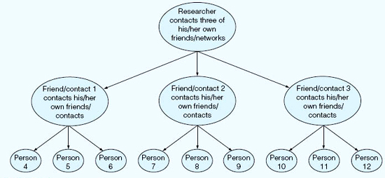
Further, if a researcher is to move beyond his or her personal contacts, to try to be more inclusive of otherwise excluded subgroups or individuals, then there is a risk having such small numbers of others as to be simply tokenism at work. Browne (2005: 53) writes that the women who participated in her research were also gatekeepers of contact to other non-heterosexual women who, for a variety of reasons (not least of which was the wish to avoid revealing too much to a friend), may not have wished to be involved. Bias can both include and exclude members of a population and a sample; it ‘can create other “hídden populations” ’ (Browne, 2005: 53) (see Figure 8.2), and the gatekeepers can protect friends by not referring them to the researcher (Heckathorn, 1997: 175).
Figure 8.2 indicates a linear, sequential method of sampling (the arrows are unidirectional). Noy (2008: 333) comments that, as the ordinal succession proceeds, the later members of the sample might have different characteristics or attributes from the earlier members of the sample, i.e. the sample is not necessarily homogeneous. This is important, as it overcomes the problem indicated earlier, where the influence of initial contacts on later contacts is high; having many waves of contacts reduces this influence (Heckathorn, 1997: 197).
Snowball sampling can be used as the main method of gaining access to people or as an auxiliary method of gaining access to people for further, in-depth data collection and exploration of issues.
In cases where access is difficult, the researcher may have to rely on volunteers, for example, personal friends, or friends of friends, or participants who reply to a newspaper advertisement, or those who happen to be interested from a particular school, or those attending courses. Sometimes this is inevitable (Morrison, 2006), as it is the only kind of sampling that is possible, and it is maybe better to have this kind of sampling than no research at all.
In these cases one has to be very cautious in making any claims for generalizability or representativeness, as volunteers may have a range of different motives for volunteering, e.g. wanting to help a friend, interest in the research, wanting to benefit society, an opportunity for revenge on a particular school or headteacher. Volunteers may be well intentioned, but they do not necessarily represent the wider population, and this would have to be made clear.
This is a feature of grounded theory. In grounded theory the sample size is relatively immaterial, as one works with the data that one has. Indeed grounded theory would argue that the sample size could be infinitely large, or, as a fall-back position, large enough to saturate the categories and issues, such that new data will not cause the theory that has been generated to be modified.
Theoretical sampling requires the researcher to have sufficient data to be able to generate and ‘ground’ the theory in the research context, however defined, i.e. to create theoretical explanation of what is happening in the situation, without having any data that do not fit the theory. Since the researcher will not know in advance how much or what range of data will be required, it is difficult, to the point of either impossibility, exhaustion or time limitations, to know in advance the sample size required. The researcher proceeds in gathering more and more data until the theory remains unchanged or until the boundaries of the context of the study have been reached, until no modifications to the grounded theory are made in light of the constant comparison method. Theoretical saturation (Glaser and Strauss, 1967: 61) occurs when no additional data are found that advance, modify, qualify, extend or add to the theory developed (see also Krueger and Casey, 2000).
Glaser and Strauss (1967: 45) write that theoretical sampling is where, during the data collection process as part of theory generation, the researcher collects data, codes the data and analyses them, and this analysis influences what data to collect next, from whom and where. The two key questions for the grounded theorist using theoretical sampling are: (a) to which groups does one turn next for data? (b) for what theoretical purposes does one seek further data? In response to (a), the authors (p. 49) suggest that the decision is based on theoretical relevance, i.e. those groups that will assist in the generation of as many properties and categories as possible.
Hence the size of the data set may be fixed by the number of participants in the organization, or the number of people to whom one has access, but the researcher has to consider that the door may have to be left open for him/her to seek further data in order to ensure theoretical adequacy and to check what has been found so far with further data (Flick et al., 2004: 170). In this case it is not always possible to predict at the start of the research just how many, and who, the researcher will need for the sampling; it becomes an iterative process.
Non-probability samples also reflect the issue that sampling can be of people but it can also be of issues. Samples of people might be selected because the researcher is concerned to address specific issues, for example, those students who misbehave, those who are reluctant to go to school, those with a history of drug dealing, those who prefer extra-curricular to curricular activities. Here it is the issue that drives the sampling, and so the question becomes not only ‘whom should I sample’ but ‘what should I sample’ (Mason, 2002: 127–32). In turn this suggests that it is not only people who may be sampled, but texts, documents, records, settings, environments, events, objects, organizations, occurrences, activities and so on.
It is often the case in qualitative research that non-probability, purposive samples are taken. However, whilst much of the discussion of probability samples is more relevant to quantitative research (though not exclusively so), and whilst much of the discussion of non-probability samples is more relevant to qualitative research (though not exclusively so), some qualitative research also raises a fundamental question about sampling. The question is this: if sampling presupposes an identifiable population from which a sample is drawn, then is it actually realistic or relevant to identify a population or its sample?
In much qualitative research the emphasis is placed on the uniqueness, the idiographic and exclusive distinctiveness of the phenomenon, group or individuals in question, i.e. they only represent themselves, and nothing or nobody else. In such cases it is perhaps unwise to talk about a ‘sample’, and more fitting to talk about a group, or individuals. How far they are representative of a wider population or group is irrelevant, as much qualitative research seeks to explore the particular group under study, not to generalize. If, in the process, other groups find that issues raised apply to them then this is a fortunate bonus rather than a necessity; in this respect it is akin to case study research.
Further, a corollary of the sympathy between qualitative research and non-probability sampling is that there are no clear rules on the size of the sample in qualitative research; size is informed by ‘fitness for purpose’. For example a case study might involve only one child (e.g. Axline, 1964), a grounded theory might continue to add samples until theoretical saturation is reached (i.e. where new data no longer add to the theory construction or themes, or their elements), an ethnography takes in the whole of the group under study, sometimes without any intention of representing a wider population (e.g. Patrick, 1973) and at other times seeking to represent some key features of a wider population (e.g. Willis, 1977).
This is not to say that there are no occasions on which, in qualitative research, a sample cannot fairly represent a population. Indeed Onwuegbuzie and Leech (2007: 240) argue that external generalizability and inferences to a whole population can feature in qualitative research, and that, as in quantitative research, this typically requires a large sample to be drawn (p. 242). The authors contrast this with internal generalizability, in which data from a subgroup of a sample seek to be generalizable to the whole sample. That said, they note (p. 249) that, many times, the purpose of the sampling is not to make generalizations, not to make comparisons, but to present unique cases that have their own, intrinsic value.
Onwuegbuzie and Leech (2007: 242) suggest that, in qualitative research, the sample size should be large enough to generate ‘thick descriptions’ (Geertz, 1973) and rich data, though not so large as to prevent this from happening due to data overload or moves towards generalizability, and not so small as to prevent theoretical saturation (discussed earlier) from being achieved. Onwuegbuzie and Leech (2007: 245) also counsel that subgroups in a sample should not be so small as to prevent data redundancy or data saturation, and, in this respect, they recommend that each subgroup should contain no fewer than three cases. As with quantitative data (discussed earlier), they note that as the number of strata increase, so will the size of the sample.
Teddlie and Tashakkori (2009: 180–1), drawing on the work of Teddlie and Yu (2007), indicate that it is commonplace for mixed methods research to use more than one kind of sample (probability, non-probability) and to use samples of different sizes, scope and types (cases: people; materials: written, oral observational; other elements in social situations: locations, times, events, etc.) within the same piece of research. This is akin to the work of Spradley (1980) on participant observation, Patton (1990) on qualitative research, and Miles and Huberman (1994) in discussing actors (participants), settings, events and processes. Even though mixed methods may be used in a piece of research, this is not to rule out the fact that, in some research, the numerical approach may predominate – with the sampling implications indicated earlier in this chapter (e.g. probability sampling and sample size calculation) – whilst in other mixed methods approaches qualitative data may predominate, with an emphasis on purposive and non-probability sampling (cf. Teddlie and Yu, 2007: 85).
Teddlie and Tashakkori (2009: 185–91) provide a useful overview of different mixed methods sampling designs (see also Chapter 1). In parallel mixed methods sampling both probability and non-probability samples are selected, running side by side simultaneously, but separate from each other, i.e. data from one sample do not influence the collection of data from the other and vice versa. Onwuegbuzie and Leech (2007: 239) add that parallel sampling designs enable comparisons to be made across two or more subgroups of a sample that are within the same level of the sample (e.g. girls and boys).
In sequential mixed methods sampling (Teddlie and Tashakkori, 2009: 185–91) one kind of sample (both probability and non-probability) precedes another and influences the proceeding sample; in other words what one gathers from an early sample will influence what one will do in the next stage with a different sample. This might mean that numerical data set the scene for in-depth interviewing, perhaps identifying extreme or deviant cases, critical cases, variables on which the results are either homogeneous or highly varied; alternatively it might mean that qualitative data (e.g. case studies or focus groups) might identify issues for exploration in a numerical survey.
In multilevel mixed methods sampling, different kinds of sample (both probability and non-probability and either separately or together) are used at different levels of units of analysis, for example: individual students, classes, schools, local authorities, regions. Onwuegbuzie and Leech (2007: 240) suggest that multilevel sampling designs enable comparisons to be made between two or more subgroups that are drawn from different levels of the study (e.g. individual students and teachers, or individual students and schools, as there is a perceptible hierarchy operating here). They add that this is facilitated by software (e.g. N-Vivo) that enables such comparative data to be collected and presented by subgroup. They also caution researchers to note that, often, a subsample from one level is not the same size as the subsample from another (p. 249), for instance there may be 30 individual students but only one or two teachers for that group of students (they note, in this context, that it is frequently the case that the levels are related, e.g. students and teachers from the same school, rather than being separate, e.g. students from one school and teachers from another).
Teddlie and Tashakkori (2009: 191) provide a worked example of a multilevel, mixed method sampling design for a school effectiveness study, in which:
at level one, students were selected by probability (random) and purposive sampling (typical cases and complete collection sampling);
at level two, teachers and classrooms were selected by probability (random and random stratified) and purposive sampling (intensity and typical case sampling);
at level three, schools were sampled using purposive samples (extreme and deviant case sampling, intensity sampling and typical case sampling);
at level four, school districts were sampled using probability sampling (cluster samples) and stratified purposive samples;
at level five, state school systems were sampled using purposive or convenience sampling.
Teddlie and Tashakkori (2009: 186) suggest that stratified purposive sampling is useful. Here the researcher identifies the different strata (e.g. subgroups) within the population under study, and then selects a limited number of cases from within each of those subgroups, ensuring that the selection of these cases is based on purposive sampling strategies (i.e. fitness for purpose), drawing on the range of purposive sampling strategies outlined earlier in this chapter. This, they aver, enables the researcher to make comparisons across groups (strata) as required. In this case the purposive sample is a subset of the probability sample (Teddlie and Yu, 2007: 93).
Teddlie and Tashakkori (2009: 186–7) also commend the use of purposeful random sampling, in which the researcher takes a random sample from a small number of cases from the population (a probability sample) that has already been drawn from a purposive sample (where the population has been chosen for a specific purpose).
Onwuegbuzie and Leech (2007: 239) introduce nested sampling designs, which enable comparisons to be made between two or more members of the same subgroup and the whole sample. The members of a subgroup represent a subsample of the whole sample (p. 246). They give the example (p. 240) of a comparison between key informants and the whole sample.
Teddlie and Tashakkori (2009: 192–3) also provide useful guidance for sampling in mixed methods research, suggesting that the sampling strategy should:
derive logically the research questions or hypotheses being investigated/tested;
be faithful to the assumptions on which the sampling strategies are based (e.g. random allocation, even distributions of characteristics in the population, etc.);
generate qualitative and quantitative data in order to answer the research questions;
enable clear inferences to be drawn from both the numerical and qualitative data;
abide by ethical principles;
be practicable (able to be done) and efficient;
enable generalizabilty of the results (and should indicate to whom the results are generalizable);
be reported in a level of detail that will enable other researchers to understand it and perhaps use it in the future.
There are several stages in planning the sampling strategy:
Stage 1: Decide whether you need a sample, or whether it is possible to have the whole population.
Stage 2: Identify the population, its important features (the sampling frame) and its size.
Stage 3: Identify the kind of sampling strategy you require (e.g. which variant of probability, non-probability or mixed methods sample you require).
Stage 4: Ensure that access to the sample is guaranteed. If not, be prepared to modify the sampling strategy (Stage 2).
Stage 5: For probability sampling, identify the confidence level and confidence intervals that you require. For non-probability sampling, identify the people whom you require in the sample.
Stage 6: Calculate the numbers required in the sample, allowing for non-response, incomplete or spoiled responses, attrition and sample mortality, i.e. build in redundancy by oversampling.
Stage 7: Decide how to gain and manage access and contact (e.g. advertisement, letter, telephone, email, personal visit, personal contacts/friends).
Stage 8: Be prepared to weight (adjust) the data, once collected.
The message from this chapter is the same as for many of the others, namely that every element of the research should not be arbitrary but planned and deliberate, and that, as before, the criterion of planning must be fitness for purpose. The selection of a sampling strategy must be governed by the criterion of suitability. The choice of which strategy to adopt must be mindful of the purposes of the research, the times-cales and constraints on the research, the research design, the methods of data collection and the methodology of the research. The sampling chosen must be appropriate for all these factors if validity is to be served.
To the question ‘how large should my sample be?’. the answer is complicated. This chapter has suggested that it all depends on:
the research purposes, questions and design;
the population size;
the confidence level and confidence interval required;
the likely response rate;
the accuracy required (the smallest sampling error sought);
the kinds of variables to be used (categorical, continuous);
the statistics to be used;
the number of strata required;
the number of variables included in the study;
the variability of the factor under study;
the kind(s) of sample (different kinds of sample within probability, non-probability and mixed methods sampling);
the representativeness of the sample;
the allowances to be made for attrition and non-response;
the need to keep proportionality in a proportionate sample;
the kind of research that is being undertaken (qualitative/quantitative/mixed methods).
Probability samples |
Non-probability samples |
Mixed methods sampling designs |
Simple random sampling |
Convenience sampling |
Parallel mixed methods sampling |
Systematic sampling |
Quota sampling |
Sequential mixed methods sampling |
Random stratified sampling |
Purposive sampling: |
Multilevel mixed methods sampling |
Cluster sampling |
Boosted sample |
Stratified purposive sampling |
Stage sampling |
Negative case sampling |
Purposeful random sampling |
Multi-phase sampling |
Typical case sampling |
Nested sampling designs |
|
Extreme/deviant case sampling |
|
|
Intensity sampling |
|
|
Maximum variation sampling |
|
|
Homogeneous sampling |
|
|
Reputational case sampling |
|
|
Revelatory case sampling |
|
|
Critical case sampling |
|
|
Politically important case sampling |
|
|
Complete collection sampling |
|
|
Theoretical sampling |
|
|
Confirming and disconfirming case sampling |
|
|
Opportunistic sampling |
|
|
Snowball sampling |
|
|
Dimensional sampling |
|
|
Volunteer sampling |
|
That said, this chapter has urged researchers to use large rather than small samples in quantitative research and sufficiently large and small samples to enable thick descriptions to be achieved. Table 8.3 presents a summary of the types of samples that we have introduced in this chapter.
 Companion Website
The companion website to the book includes PowerPoint slides for this chapter, which list the structure of the chapter and then provide a summary of the key points in each of its sections. This resource can be found online at www.routledge.com/textbooks/cohen7e.