frequencies, percentages and crosstabulations
Descriptive statistics |
CHAPTER 35 |
This chapter introduces descriptive statistics. Descriptive statistics do what they say: they describe, so that researchers can then analyse and interpret what these descriptions mean. This chapter introduces some key descriptive statistics and how to use them. This includes:
frequencies, percentages and crosstabulations
measures of central tendency and dispersal
taking stock
correlations and measures of association
partial correlations
reliability
Descriptive statistics include frequencies, measures of dispersal (standard deviation), measures of central tendency (means, modes, medians), standard deviations, crosstabulations and standardized scores. We address all these in this chapter, with the exception of standardized scores, which we keep for Chapter 36.
In descriptive statistics much is made of visual techniques of data presentation. Hence frequencies and percentages, and forms of graphical presentation are often used. A host of graphical forms of data presentation are available in software packages, including, for example:
frequency and percentage tables;
bar charts (for nominal and ordinal data);
histograms (for continuous – interval and ratio – data);
line graphs;
pie charts;
high and low charts;
scatterplots;
stem and leaf displays;
boxplots (box and whisker plots).
With most of these forms of data display there are various permutations of the ways in which data are displayed within the type of chart or graph chosen. Whilst graphs and charts may look appealing, it is often the case that they tell the reader no more than could be seen in a simple table of figures, and figures take up less space in a report. Pie charts, bar charts and histograms are particularly prone to this problem, and the data in them could be placed more succinctly into tables. Clearly the issue of fitness for audience is important here: some readers may find charts more accessible and able to be understood than tables of figures, and this is important. Other charts and graphs can add greater value than tables, for example line graphs, boxplots and scatterplots with regression lines, and we would suggest that these are helpful. Here is not the place to debate the strengths and weaknesses of each type, though the following list presents some guides:
bar charts are useful for presenting categorical and discrete data, highest and lowest;
avoid using a third dimension (e.g. depth) in a graph when it is unnecessary; a third dimension to a graph must provide additional information;
histograms are useful for presenting continuous data;
line graphs are useful for showing trends, particularly in continuous data, for one or more variables at a time;
multiple line graphs are useful for showing trends in continuous data on several variables in the same graph;
pie charts and bar charts are useful for showing proportions;
interdependence can be shown through crosstabulations (discussed below);
boxplots are useful for showing the distribution of values for several variables in a single chart, together with their range and medians;
stacked bar charts are useful for showing the frequencies of different groups within a specific variable for two or more variables in the same chart;
scatterplots are useful for showing the relationship between two variables or several sets of two or more variables on the same chart.
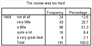
At a simple level one can present data in terms of frequencies and percentages, as shown in Table 35.1 (a piece of datum about a course evaluation). From this simple table we can tell that:
191 people completed the item;
most respondents thought that the course was ‘a little’ too hard (with a clear modal score of 98, i.e. 51.3%); the modal score is that category or score which is given by the highest number of respondents;
the results were skewed, with only 10.5 per cent being in the categories ‘quite a lot’ and ‘a very great deal’;
more people thought that the course was ‘not at all too hard’ than thought that the course was ‘quite a lot’ or ‘a very great deal’ too hard;
overall the course appears to have been slightly too difficult but not much more.
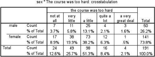
Let us imagine that we wished to explore this piece of datum further. We may wish to discover, for example, the voting on this item by males and females. This can be presented in a simple crosstabulation, following the convention of placing the nominal data (male and female) in rows and the ordinal data (the five-point scale) in the columns (or independent variables as row data and dependent variables as column data). A crosstabulation is simply a presentational device, whereby one variable is presented in relation to another, with the relevant data inserted into each cell (automatically generated by software packages, such as SPSS) (Table 35.2).
Table 35.2 shows that, of the total sample, nearly three times more females (38.2%) than males (13.1%) thought that the course was ‘a little’ too hard, between two-thirds and three-quarters more females (19.9%) than males (5.8%) thought that the course was a ‘very little’ too hard, and around three times more males (1.6%) than females (0.5%) thought that the course was ‘a very great deal’ too hard. However, one also has to observe that the size of the two subsamples was uneven. Around three-quarters of the sample was female (73.8%) and around one-quarter (26.2%) was male.
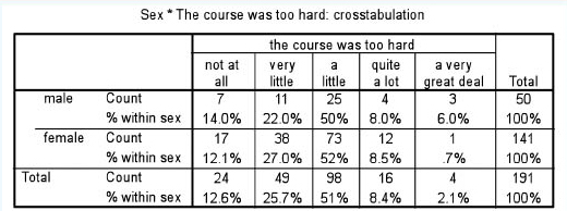
There are two ways to overcome the problem of uneven subsample sizes. One is to adjust the sample, in this case by multiplying up the subsample of males by an exact figure in order to make the two subsamples the same size (141/50 = 2.82). Another way is to examine the data by each row rather than by the overall totals, i.e. to examine the proportion of males voting such-and-such, and, separately, the proportion of females voting for the same categories of the variable, as shown in Table 35.3.
If you think that these two calculations and recalculations are complicated or difficult (overall-percentaged totals and row-percentaged totals), then be reassured: many software packages, e.g. SPSS (the example used here) will do this at one keystroke.
In this second table (Table 35.3) one can observe that:
there was consistency in the voting by males and females in terms of the categories ‘a little’ and ‘quite a lot’;
more males (6%) than females (0.7%) thought that the course was ‘a very great deal’ too hard;
a slightly higher percentage of females (91.1%: {12.1% + 27% + 52%}) than males (86%: {14% + 22% + 50%}) indicated, overall, that the course was not too hard;
the overall pattern of voting by males and females was similar, i.e. for both males and females the strong to weak categories in terms of voting percentages were identical.
We would suggest that this second table is more helpful than the first table, as, by including the row percentages, it renders fairer the comparison between the two groups: males and females. Further, we would suggest that it is usually preferable to give both the actual frequencies and percentages, but to make the comparisons by percentages. We say this, because it is important for the reader to know the actual numbers used. For example, in the first table (Table 35.2), if we were simply to be given the percentage of males voting that the course was a ‘very great deal’ too hard (1.6%), as course planners we might worry about this. However, when we realize that 1.6% is actually only three out of 141 people then we might be less worried. Had the 1.6% represented, say, 50 people of a sample, then this would have given us cause for concern. Percentages on their own can mask the real numbers, and the reader needs to know the real numbers.
It is possible to comment on particular cells of a crosstabulated matrix in order to draw attention to certain factors (e.g. the very high 52% in comparison to its neighbour 8.5% in the voting of females in Table 35.3). It is also useful, on occasions, to combine data from more than one cell, as we have done in the list above. For example, if we combine the data from the males in the categories ‘quite a lot’ and ‘a very great deal’ (8% + 6% = 14%) we can observe that not only is this equal to the category ‘not at all’, but it contains fewer cases than any of the other single categories for the males, i.e. the combined category shows that the voting for the problem of the course being too difficult is still very slight.
Combining categories can be useful in showing the general trends or tendencies in the data. For example, in Tables 35.1–35.3, combining the measures ‘not at all’, ‘very little’ and ‘a little’ indicates that it is only a very small problem of the course being too hard, i.e. generally speaking the course was not too hard.
TABLE 35.4 RATING SCALE OF AGREEMENT AND DISAGREEMENT
Strongly disagree |
Disagree |
Neither agree nor disagree |
Agree |
Strongly agree |
30 |
40 |
70 |
20 |
40 |
15% |
20% |
35% |
10% |
20% |
Combining categories can also be useful in rating scales of agreement to disagreement. For example, consider the results in Table 35.4 in relation to a survey of 200 people on a particular item. There are several ways of interpreting the table, for example: (a) more people ‘strongly agreed’ (20%) than ‘strongly disagreed’ (15%); (b) the modal score was for the central neutral category (a central tendency) of ‘neither agree nor disagree’. However one can go further. If one wishes to ascertain an overall indication of disagreement and agreement, then adding together the two disagreement categories yields 35% (15% + 20%) and adding together the two agreement categories yields 30% (10% + 20%), i.e. there was more disagreement than agreement, despite the fact that more respondents ‘strongly agreed’ than ‘strongly disagreed’, i.e. the strength of agreement and disagreement has been lost. By adding together the two disagreement and agreement categories it gives us a general rather than a detailed picture; this may be useful for our purposes. However, if we do this then we also have to draw attention to the fact that the total of the two disagreement categories (35%) is the same as the total in the category ‘neither agree nor disagree’, in which case one could suggest that the modal category of ‘neither agree nor disagree’ has been superseded by bi-modality, with disagreement being one modal score and ‘neither agree nor disagree’ being the other.
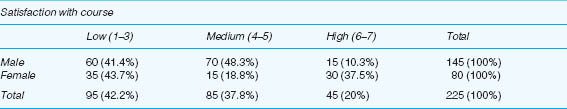
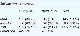
Combining categories can be useful though it is not without its problems, for example let us consider three tables (Tables 35.5–35.7). The first presents the overall results of an imaginary course evaluation, in which three levels of satisfaction have been registered (low, medium, high) (Table 35.5). Here one can observe that the modal category is ‘low’ (95 votes, 42.2%) and the lowest category is ‘high’ (45 votes, 20%), i.e. overall the respondents are dissatisfied with the course. The females seem to be more satisfied with the course than the males, if the category ‘high’ is used as an indicator, and the males seem to be more moderately satisfied with the course than the females.
However, if one combines categories (low and medium) then a different story could be told, as in Table 35.6. By looking at the percentages, here it appears that the females are more satisfied with the course overall than males, and that the males are more dissatisfied with the course than females.
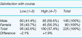
However, if one were to combine categories differently (medium and high) then a different story again could be told, as in Table 35.7. By looking at the percentages, here it appears that there is not much difference between the males and the females, and that both males and females are highly satisfied with the course.
At issue here is the notion of combining categories, or collapsing tables, and we advocate great caution in doing this. Sometimes it can provide greater clarity, and sometimes it can distort the picture. In the example here it is wiser to keep with the original table (Table 35.5) rather than collapsing it into fewer categories.
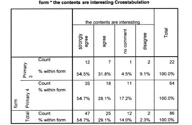
Crosstabulations used for categorical data can be bivariate (two variables presented), for example Table 35.8, in which two forms of primary students (Primary 3 and Primary 4) are asked how interesting they find a course. The rows are the nominal, categorical variable and the columns are the values of the ordinal variable. This is a commonplace organization.
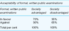
Let us give another example, let us suppose that we wished to examine the views of parents from socially advantaged and disadvantaged backgrounds of primary school children on traditional school examinations (in favour/against), using simple dichotomous variables (two values only in each variable). Table 35.9 presents the results. It shows us clearly that parents from socially advantaged backgrounds are more in favour of formal, written public examinations than those from socially disadvantaged backgrounds.
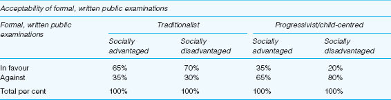
Additionally, a trivariate crosstabulation can be constructed (and SPSS enables researchers to do this), with three variables included. In the example here, let us say that we are interested in their socio-economic status (socially advantaged/socially disadvantaged) and their philosophies of education (traditionalist/child-centred). Our results appear as in Table 35.10.
The results here are almost the reverse of Table 35.9: now the socially advantaged are more likely than socially disadvantaged parents to favour forms of assessment other than formal, written public examinations, and socially disadvantaged parents are more likely than socially advantaged parents to favour formal, written public examinations. The educational philosophies of each of the two groups (socially advantaged and socially disadvantaged) have dramatically altered the scenario. A trivariate analysis can give greater subtlety to the data and their analysis. (They can be used as control variables, and we address this in the discussion of correlations.)
The central tendency of a set of scores is the way in which they tend to cluster round the middle of a set of scores, or where the majority of scores are located. For categorical data the measure of central tendency is the mode: that score which is given by the most people, that score which has the highest frequency (there can be more than one mode: if there are two clear modal scores then this is termed ‘bimodal’; if there are three then this is termed ‘tri-modal’). For continuous data (ratio data), in addition to the mode, the researcher can calculate the mean (the average score) and the median: the midpoint score of a range of data; half of the scores fall above it and half below it (the median is also sometimes used for ordinal data). If there is an even number of observations then the median is the average of the two middle scores. We cannot calculate the median score for nominal data, as the data have to be ranked-ordered from the lowest to the highest in terms of the quantity of the variable under discussion. Measures of central tendency are used with univariate data, and indicate the typical score (the mode), the middle score (the median) and the average score (the mean).
As a general rule, the mean is a useful statistic if the data are not skewed (i.e. if they are not bunched at one end or another of a curve of distribution) or if there are no outliers that may be exerting a disproportionate effect. One has to recall that the mean, as a statistical calculation only, can sometime yield some strange results, for example fractions of a person!
The median is useful for ordinal data, but, to be meaningful, there have to be many scores rather than just a few. The median overcomes the problem of outliers, and hence is useful for skewed results. The modal score is useful for all scales of data, particularly nominal and ordinal data, i.e. discrete and categorical data, rather than continuous data, and it is unaffected by outliers, though it is not strong if there are many values and many scores which occur with similar frequency (i.e. if there are only a few points on a rating scale).
Are scores widely dispersed around the mean, do they cluster close to the mean, or are they at some distance from the mean? The measures used to determine this are measures of dispersal. If we have interval and ratio data then, in addition to the modal score and crosstabulations, we can calculate the mean (the average) and the standard deviation. The standard deviation is the average distance that each score is from the mean, i.e. the average difference between each score and the mean, and how much the scores, as a group, deviate from the mean. It is a standardized measure of dispersal. For small samples (fewer than 30 scores), or for samples rather than populations, it is calculated as:

where
d 2 = the deviation of the score from the mean (average), squared
∑ = the sum of
N = the number of cases
For populations rather than samples, it is calculated as:
A low standard deviation indicates that the scores cluster together, whilst a high standard deviation indicates that the scores are widely dispersed. This is calculated automatically by software packages such as SPSS at the simple click of a single button.
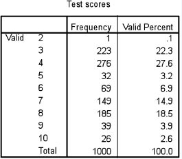
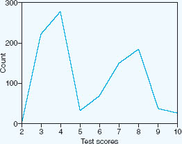
Let us imagine that we have the test scores for 1,000 students, on a test that was marked out of ten, as shown in Table 35.11. Here we can calculate that the average score was 5.48. We can also calculate the standard deviation. In the example here the standard deviation in the example of scores was 2.134. What does this tell us? First, it suggests that the marks were not very high (an average of 5.48). Second, it tells us that there was quite a variation in the scores. Third, one can see that the scores were unevenly spread, indeed there was a high cluster of scores around the categories of 3 and 4, and another high cluster of scores around the categories 7 and 8. This is where a line graph could be useful in representing the scores, as it shows two peaks clearly, as in Figure 35.1.
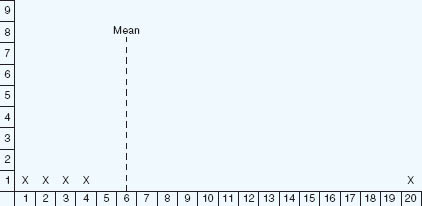
It is important to report the standard deviation. For example, let us consider the following. Look at these three sets of numbers:
(1) |
1 |
2 |
3 |
4 |
20 |
mean = 6 |
(2) |
1 |
2 |
6 |
10 |
11 |
mean = 6 |
(3) |
5 |
6 |
6 |
6 |
7 |
mean = 6 |
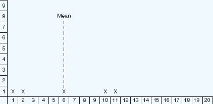
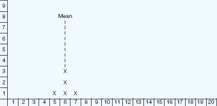
If we were to plot these points on to three separate graphs we would see very different results (Figures 35.2–35.4).
Figure 35.2 shows the mean being heavily affected by the single score of 20 (an ‘outlier’ – an extreme score a long way from the others); in fact all the other four scores are some distance below the mean. The score of 20 is exerting a disproportionate effect on the data and on the mean, raising it. Some statistical packages (e.g. SPSS) can take out outliers. If the data are widely spread then it may be more suitable not to use the mean but to use the median score; SPSS performs this automatically at a click of a button.
Figure 35.3 shows one score actually on the mean but the remainder some distance away from it. The scores are widely dispersed and the shape of the graph is flat (a platykurtic distribution).
Figure 35.4 shows the scores clustering very tightly around the mean, with a very peaked shape to the graph (a leptokurtic distribution).
The point at stake is this: it is not enough simply to calculate and report the mean; for a fuller picture of the data we need to look at the dispersal of scores. For this we require the statistic of the standard deviation, as this will indicate the range and degree of dispersal of the data, though the standard deviation is susceptible to the disproportionate effects of outliers. Some scores will be widely dispersed (Figure 35.2), others will be evenly dispersed (Figure 35.3), and others will be bunched together (Figure 35.4). A high standard deviation will indicate a wide dispersal of scores, a low standard deviation will indicate clustering or bunching together of scores.
A second way of measuring dispersal is to calculate the range, which is the difference between the lowest (minimum) score and the highest (maximum) score in a set of scores. This incorporates extreme scores, and is susceptible to the distorting effect of outliers: a wide range may be given if there are outliers, and if these outliers are removed then the range may be much reduced. Further, the range tells the researcher nothing about the distributions within the range.
Another measure of dispersion is the interquartile range. If we arrange a set of scores in order, from the lowest to the highest, then we can divide that set of scores into four equal parts: the lowest quarter (quartile) that contains the lowest quarter of all the scores, the lower middle quartile, the upper middle quartile, and the highest quarter (quartile) that contains the highest quarter of the scores. The interquartile range is the difference between the first quartile and the third quartile, or, more precisely the difference between the 25th and the 75th percentile, i.e. the middle 50 per cent of scores (the second and third quartiles). This, thereby, ignores extreme scores and, unlike the simple range, does not change significantly if the researcher adds some scores that are some distance away from the average. For example let us imagine that we have a set of test scores thus, ordered into quartiles:
FIRST QUARTILE |
SECOND QUARTILE |
THIRD QUARTILE |
FOURTH QUARTILE |
40 41 43 47 |
50 55 58 63 |
65 70 75 77 |
83 86 90 93 |
The interquartile range is 65–47 = 18. There are other ways of calculating the interquartile range (e.g. the difference between the medians of the first and third quartiles), and the reader may wish to explore these.
Though there are several ways of calculating dispersal, by far the most common is the standard deviation.
What we do with simple frequencies and descriptive data depends on the scales of data that we have (nominal, ordinal, interval and ratio). For all four scales we can calculate frequencies and percentages, and we can consider presenting these in a variety of forms. We can also calculate the mode and present crosstabulations, both bivariate and trivariate crosstabulations. We can consider combining categories and collapsing tables into smaller tables, providing that the sensitivity of the original data has not been lost. We can calculate the median score, which is particularly useful if the data are spread widely or if there are outliers. For interval and ratio data we can also calculate the mean and the standard deviation; the mean yields an average and the standard deviation indicates the range of dispersal of scores around that average, i.e. to see whether the data are widely dispersed (e.g. in a platykurtic distribution), or close together with a distinct peak (in a leptokurtic distribution). We can use other measures of dispersal such as the range and the interquartile range. In examining frequencies and percentages one also has to investigate whether the data are skewed, i.e. over-represented at one end of a scale and under-represented at the other end. A positive skew has a long tail at the positive end and the majority of the data at the negative end, and a negative skew has a long tail at the negative end and the majority of the data at the positive end.
Much educational research is concerned with establishing interrelationships among variables. We may wish to know, for example, how delinquency is related to social class background; whether an association exists between the number of years spent in full-time education and subsequent annual income; whether there is a link between personality and achievement. What, for example, is the relationship, if any, between membership of a public library and social class status? Is there a relationship between social class background and placement in different strata of the secondary school curriculum? Is there a relationship between gender and success/failure in ‘first-time’ driving test results?
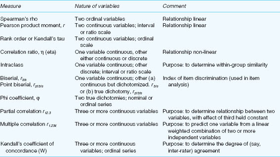
There are several simple measures of association readily available to the researcher to help him or her test these sorts of relationships. We have selected the most widely used ones here and set them out in Table 35.12.
Of these, the two most commonly used correlations are the Spearman rank order correlation for ordinal data and the Pearson product moment correlation for interval and ratio data, and we advise readers to use these as the main kinds of correlation statistics. At this point it is pertinent to say a few words about some of the terms used in Table 35.12 to describe the nature of variables. Cohen and Holliday (1982, 1996) provide worked examples of the appropriate use and limitations of the correlational techniques outlined in Table 35.12, together with other measures of association such as Kruskal’s gamma, Somer’s d and Guttman’s lambda.
Look at the words used at the top of the table to explain the nature of variables in connection with the measure called the Pearson product moment, r. The variables, we learn, are ‘continuous’ and at the ‘interval’ or the ‘ratio’ scale of measurement.
A continuous variable is one that, theoretically at least, can take any value between two points on a scale. Weight, for example, is a continuous variable; so too is time, so also is height. Weight, time and height can take on any number of possible values between nought and infinity, the feasibility of measuring them across such a range being limited only by the variability of suitable measuring instruments.
Turning again to Table 35.12, we read in connection with the next measure shown there (rank order or Kendall’s tau) that the two continuous variables are at the ordinal scale of measurement.
The variables involved in connection with the phi coefficient measure of association (halfway down Table 35.12) are described as ‘true dichotomies’ and at the nominal scale of measurement. Truly dichotomous variables (such as sex or driving test result) can take only two values (male or female; pass or fail).
To conclude our explanation of terminology, readers should note the use of the term ‘discrete variable’ in the description of the fourth correlation ratio (eta) in Table 35.12. We said earlier that a continuous variable can take on any value between two points on a scale. A discrete variable, however, can only take on numerals or values that are specific points on a scale. The number of players in a football team is a discrete variable. It is usually 11; it could be fewer than 11, but it could never be seven and a quarter!
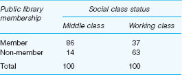
The percentage difference is a simple asymmetric measure of association. An asymmetric measure is a measure of one-way association. That is to say, it estimates the extent to which one phenomenon implies the other but not vice versa. Gender, as we shall see shortly, may imply driving test success or failure. The association could never be the other way round! Measures which are concerned with the extent to which two phenomena imply each other are referred to as symmetric measures. Table 35.13 reports the percentage of public library members by their social class origin.
What can we discover from the data set out in Table 35.13? By comparing percentages in different columns of the same row, we can see that 49% more middle-class persons are members of public libraries than working-class persons. By comparing percentages in different rows of the same columns we can see that 72% more middle-class persons are members rather than non-members. The data suggest, do they not, an association between the social class status of individuals and their membership of public libraries.
A second way of making use of the data in Table 35.13 involves the computing of a percentage ratio (%R). Look, for example, at the data in the second row of Table 35.13. By dividing 63 by 14 (%R = 4.5) we can say that four and a half times as many working-class persons are not members of public libraries as are middle-class persons.
The percentage difference ranges from 0% when there is complete independence between two phenomena to 100% when there is complete association in the direction being examined. It is straightforward to calculate and simple to understand. Notice, however, that the percentage difference as we have defined it can only be employed when there are only two categories in the variable along which we percentage and only two categories in the variable in which we compare. In SPSS, using the ‘Crosstabs’ command can yield percentages, and we indicate this in the website manual that accompanies this volume.
In connection with this issue, on the accompanying website we discuss the phi coefficient, the correlation coefficient tetrachoric r (rt), the contingency coefficient C, and combining independent significance tests of partial relations.
In our discussion of the principal correlational techniques shown in Table 35.12, three are of special interest to us and these form the basis of much of the rest of the chapter. They are the Pearson product moment correlation coefficient, multiple correlation and partial correlation.
Correlational techniques are generally intended to answer three questions about two variables or two sets of data. First, ‘Is there a relationship between the two variables (or sets of data)?’ If the answer to this question is ‘yes’, then two other questions follow: ‘What is the direction of the relationship?’ and ‘What is the magnitude?’
Relationship in this context refers to any tendency for the two variables (or sets of data) to vary consistently. Pearson’s product moment coefficient of correlation, one of the best-known measures of association, is a statistical value ranging from –1.0 to + 1.0 and expresses this relationship in quantitative form. The coefficient is represented by the symbol r.
Where the two variables (or sets of data) fluctuate in the same direction, i.e. as one increases so does the other, or as one decreases so does the other, a positive relationship is said to exist. Correlations reflecting this pattern are prefaced with a plus sign to indicate the positive nature of the relationship. Thus, +1.0 would indicate perfect positive correlation between two factors, as with the radius and diameter of a circle, and + 0.80 a high positive correlation, as between academic achievement and intelligence, for example. Where the sign has been omitted, a plus sign is assumed.
A negative correlation or relationship, on the other hand, is to be found when an increase in one variable is accompanied by a decrease in the other variable. Negative correlations are prefaced with a minus sign. Thus, –1.0 would represent perfect negative correlation, as between the number of errors children make on a spelling test and their score on the test, and –0.30 a low negative correlation, as between absenteeism and intelligence, say. There is no other meaning to the signs used; they indicate nothing more than which pattern holds for any two variables (or sets of data).
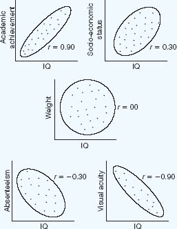
Generally speaking, researchers tend to be more interested in the magnitude of an obtained correlation than they are in its direction. Correlational procedures have been developed so that no relationship whatever between two variables is represented by zero (or 0.00), as between body weight and intelligence, possibly. This means that a person’s performance on one variable is totally unrelated to her performance on a second vari able. If she is high on one, for example, she is just as likely to be high or low on the other. Perfect correlations of +1.00 or –1.00 are rarely found and, as we shall see, most coeffi-cients of correlation in social research are around +0.50 or less. The correlation coefficient may be seen then as an indication of the predictability of one variable given the other: it is an indication of covariation. The relationship between two variables can be examined visually by plotting the paired measurements on graph paper with each pair of observations being represented by a point. The resulting arrangement of points is known as a scatterplot and enables us to assess graphically the degree of relationship between the characteristics being measured. Figure 35.5 gives some examples of scatterplots in the field of educational research.
Whilst correlations are widely used in research, and they are straightforward to calculate and to interpret, the researcher must be aware of four caveats in undertaking correlational analysis:
i do not assume that correlations imply causal relationships (i.e. simply because having large hands appears to correlate with having large feet does not imply that having large hands causes one to have large feet);
ii there is a need to be alert to a Type I error – not supporting the null hypothesis when it is in fact true;
iii there is a need to be alert to a Type II error – supporting the null hypothesis when it is in fact not true;
iv statistical significance must be accompanied by an indication of effect size.
In SPSS a typical print-out of a correlation coefficient is given in Table 35.14. In this fictitious example using 1,000 cases there are four points to note:
1 The cells of data to the right of the cells containing the figure 1 are the same as the cells to the left of the cells containing the figure 1, i.e. there is a mirror image, and, if very many more variables were being correlated then, in fact, one would have to decide whether to look at only the variables to the right of the cell with the figure 1 (the perfect correlation, since it is one variable being correlated with itself ), or to look at the cells to the left of the figure 1.
2 In each cell where one variable is being correlated with a different variable there are three figures: the top figure gives the correlation coefficient, the middle figure gives the significance level and the lowest figure gives the sample size.
3 SPSS marks with an asterisk those correlations which are statistically significant.
4 All the correlations are positive, since there are no negative coefficients given.
What these tables give us is the magnitude of the correlation (the coefficient), the direction of the correlation (positive and negative), and the significance level. The correlation coefficient can be taken as the effect size. The significance level, as mentioned earlier, is calculated automatically by SPSS, based on the coefficient and the sample size: the greater the sample size, the lower the coefficient of correlation has to be in order to be statistically significant, and, by contrast, the smaller the sample size, the greater the coefficient of correlation has to be in order to be statistically significant.
In reporting correlations one has to report the test used, the coefficient, the direction of the correlation (positive or negative) and the significance level (if considered appropriate). For example, one could write:
Using the Pearson product moment correlation, a statistically significant correlation was found between students’ attendance at school and their examination performance (r = 0.87, ρ = 0.035). Those students who attended school the most tended to have the best examination performance, and those who attended the least tended to have the lowest examination performance.
Alternatively, there may be occasions when it is important to report when a correlation has not been found, for example:
There was no statistically significant correlation found between the amount of time spent on homework and examination performance (r = 0.37, ρ = 0.43).
In both these examples of reporting, exact significance levels have been given, assuming that SPSS has calculated these. An alternative way of reporting the significance levels (as appropriate) are: ρ < 0.05; ρ < 0.01; ρ < 0.001; ρ = 0.05; ρ = 0.01, ρ = 0.001. In the case of statistical significance not having been found one could report this as ρ > 0.05 or ρ = N.S.
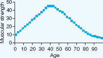
The correlations discussed so far have assumed linearity, that is the more we have of one property, the more (or less) we have of another property, in a direct positive or negative relationship. A straight line can be drawn through the points on the scatterplots (a regression line). However, linearity cannot always be assumed. Consider the case, for example, of stress: a little stress might enhance performance (‘setting the adrenalin running’) positively, whereas too much stress might lead to a downturn in performance. Where stress enhances performance there is a positive correlation, but when stress debilitates performance there is a negative correlation. The result is not a straight line of correlation (indicating linearity) but a curved line (indicating curvilinearity). This can be shown graphically, as shown in Figure 35.6. It is assumed here, for the purposes of the example, that muscular strength can be measured on a single scale. It is clear from the graph that muscular strength increases from birth until 50 years, and thereafter it declines as muscles degenerate. There is a positive correlation between age and muscular strength on the left-hand side of the graph and a negative correlation on the right-hand side of the graph, i.e. a curvilinear correlation can be observed.
Hopkins et al. (1996: 92) provide another example of curvilinearity: room temperature and comfort. Raising the temperature a little can make for greater comfort – a positive correlation – whilst raising it too greatly can make for discomfort – a negative correlation. Many correlational statistics assume linearity (e.g. the Pearson product moment correlation). However, rather than using correlational statistics arbitrarily or blindly, the researcher will need to consider whether, in fact, linearity is a reasonable assumption to make, or whether a curvilinear relationship is more appropriate (in which case more sophisticated statistics will be needed, e.g. η (‘eta’)) (Glass and Hopkins, 1996, section 8.7; Cohen and Holliday, 1996: 84; Fowler et al., 2000: 81–9) or mathematical procedures will need to be applied to transform non-linear relations into linear relations. Examples of curvilinear relationships might include:
pressure from the principal and teacher performance;
pressure from the teacher and student achievement;
degree of challenge and student achievement;
assertiveness and success;
age and muscular strength;
age and physical control;
age and concentration;
age and sociability;
age and cognitive abilities.
Hopkins et al. (1996) suggest that the variable ‘age’ frequently has a curvilinear relationship with other variables. The authors also point out (p. 92) that poorly constructed tests can give the appearance of curvilinearity if the test is too easy (a ‘ceiling effect’ where most students score highly) or if it is too difficult, but that this curvilinearity is, in fact, spurious, as the test does not demonstrate sufficient item difficulty or discriminability.
In planning correlational research, then, attention will need to be given to whether linearity or curvilinearity is to be assumed.
The coefficient of correlation, then, tells us something about the relations between two variables. Other measures exist, however, which allow us to specify relationships when more than two variables are involved. These are known as measures of ‘multiple correlation’ and ‘partial correlation’.
Multiple correlation measures indicate the degree of association between three or more variables simultaneously. We may want to know, for example, the degree of association between delinquency, social class background and leisure facilities. Or we may be interested in finding out the relationship between academic achievement, intelligence and neuroticism. Multiple correlation, or ‘regression’ as it is sometimes called, indicates the degree of association between n variables. It is related not only to the correlations of the independent variable with the dependent variables, but also to the intercorrelations between the dependent variables.
Partial correlation aims at establishing the degree of association between two variables after the influence of a third has been controlled or partialled out. Guilford and Fruchter (1973) define a partial correlation between two variables as one which nullifies the effects of a third variable (or a number of variables) on the variables being correlated. They give the example of correlation between the height and weight of boys in a group whose age varies, where the correlation would be higher than the correlation between height and weight in a group comprised of boys of only the same age. Here the reason is clear – because some boys will be older they will be heavier and taller. Age, therefore, is a factor that increases the correlation between height and weight. Of course, even with age held constant, the correlation would still be positive and significant because, regardless of age, taller boys often tend to be heavier.
Consider, too, the relationship between success in basketball and previous experience in the game. Suppose, also, that the presence of a third factor, the height of the players, was known to have an important influence on the other two factors. The use of partial correlation techniques would enable a measure of the two primary variables to be achieved, freed from the influence of the secondary variable.
Correlational analysis is simple and involves collecting two or more scores on the same group of subjects and computing correlation coefficients. Many useful studies have been based on this simple design. Those involving more complex relationships, however, utilize multiple and partial correlations in order to provide a clearer picture of the relationships being investigated.
One final point: it is important to stress again that correlations refer to measures of association and do not necessarily indicate causal relationships between variables. Correlation does not imply cause.
Once a correlation coefficient has been computed, there remains the problem of interpreting it. A question often asked in this connection is how large should the coefficient be for it to be meaningful. The question may be approached in three ways: by examining the strength of the relationship; by examining the statistical significance of the relationship; and by examining the square of the correlation coefficient.
Inspection of the numerical value of a correlation coefficient will yield clear indication of the strength of the relationship between the variables in question. Low or near zero values indicate weak relationships, while those nearer to +1 or –1 suggest stronger relationships. Imagine, for instance, that a measure of a teacher’s success in the classroom after five years in the profession is correlated with her final school experience grade as a student and that it was found that r = +0.19. Suppose now that her score on classroom success is correlated with a measure of need for professional achievement and that this yielded a correlation of 0.65. It could be concluded that there is a stronger relationship between success and professional achievement scores than between success and final student grade.
Where a correlation coefficient has been derived from a sample and one wishes to use it as a basis for inference about the parent population, the statistical significance of the obtained correlation must be considered. Statistical significance, when applied to a correlation coefficient, indicates whether or not the correlation is different from zero at a given level of confidence. As we have seen earlier, a statistically significant correlation is indicative of an actual relationship rather than one due entirely to chance. The level of statistical significance of a correlation is determined to a great extent by the number of cases upon which the correlation is based. Thus, the greater the number of cases, the smaller the correlation need be to be significant at a given level of confidence.
Exploratory relationship studies are generally interpreted with reference to their statistical significance, whereas prediction studies depend for their efficacy on the strength of the correlation coefficients. These need to be considerably higher than those found in exploratory relationship studies and for this reason rarely invoke the concept of significance.
The third approach to interpreting a coefficient is provided by examining the square of the coefficient of correlation, r2. This shows the proportion of variance in one variable that can be attributed to its linear relationship with the second variable. In other words, it indicates the amount the two variables have in common. If, for example, two variables A and B have a correlation of 0.50, then (0.50)2 or 0.25 of the variation shown by the B scores can be attributed to the tendency of B to vary linearly with A. Figure 35.7 shows graphically the common variance between reading grade and arithmetic grade having a correlation of 0.65.
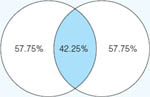
FIGURE 35.7 Visualization of correlation of 0.65 between reading grade and arithmetic grade
Source: Fox, 1969
There are three cautions to be borne in mind when one is interpreting a correlation coefficient. First, a coefficient is a simple number and must not be interpreted as a percentage. A correlation of 0.50, for instance, does not mean 50 per cent relationship between the variables. Further, a correlation of 0.50 does not indicate twice as much relationship as that shown by a correlation of 0.25. A correlation of 0.50 actually indicates more than twice the relationship shown by a correlation of 0.25. In fact, as coefficients approach +1 or –1, a difference in the absolute values of the coefficients becomes more important than the same numerical difference between lower correlations would be.
Second, a correlation does not necessarily imply a cause-and-effect relationship between two factors, as we have previously indicated. It should not therefore be interpreted as meaning that one factor is causing the scores on the other to be as they are. There are invariably other factors influencing both variables under consideration. Suspected cause-and-effect relationships would have to be confirmed by subsequent experimental study.
Third, a correlation coefficient is not to be interpreted in any absolute sense. A correlational value for a given sample of a population may not necessarily be the same as that found in another sample from the same population. Many factors influence the value of a given correlation coefficient and if researchers wish to extrapolate to the populations from which they drew their samples they will then have to test the significance of the correlation.
We now offer some general guidelines for interpreting correlation coefficients. They are based on Borg’s (1963) analysis and assume that the correlations relate to a hundred or more subjects.
Correlations ranging from 0.20 to 0.35
Correlations within this range show only very slight relationship between variables although they may be statistically significant. A correlation of 0.20 shows that only 4 per cent ({0.20 × 0.20} × 100) of the variance is common to the two measures. Whereas correlations at this level may have limited meaning in exploratory relationship research, they are of no value in either individual or group prediction studies.
Correlations ranging from 0.35 to 0.65
Within this range, correlations are statistically significant beyond the 1 per cent level. When correlations are around 0.40, crude group prediction may be possible. As Borg (1963) notes, correlations within this range are useful, however, when combined with other correlations in a multiple regression equation. Combining several correlations in this range in some cases can yield individual predictions that are correct within an acceptable margin of error. Correlations at this level used singly are of little use for individual prediction because they yield only a few more correct predictions than could be accomplished by guessing or by using some chance selection procedure.
Correlations ranging from 0.65 to 0.85
Correlations within this range make possible group predictions that are accurate enough for most purposes. Nearer the top of the range, group predictions can be made very accurately, usually predicting the proportion of successful candidates in selection problems within a very small margin of error. Near the top of this correlation range individual predictions can be made that are considerably more accurate than would occur if no such selection procedures were used.
Correlations over 0.85
Correlations as high as this indicate a close relationship between the two variables correlated. A correlation of 0.85 indicates that the measure used for prediction has about 72 per cent variance in common with the performance being predicted. Prediction studies in education very rarely yield correlations this high. When correlations at this level are obtained, however, they are very useful for either individual or group prediction.
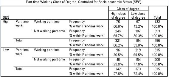
Many researchers wish to control for the effects of other variables. As was discussed in Chapter 4, controlling for the effects of variables means holding them constant whilst manipulating other variables. Let us imagine that we have 1,000 students in a survey, and that we wish to investigate the effects of working part time on their degree classification (high/low) after we have controlled for the effects of socio-economic status (high/low).
First, a crosstabulation can be calculated (e.g. in SPSS), controlled for socio-economic status, which indicates the distributions of the categories, set out by part-time work and socio-economic status as the row variables (and with the class of degree as the column variable), as in Table 35.15.
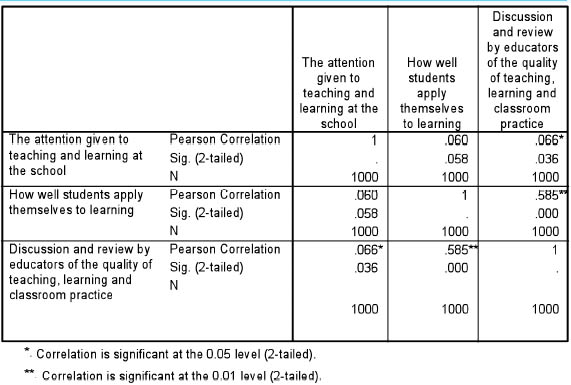
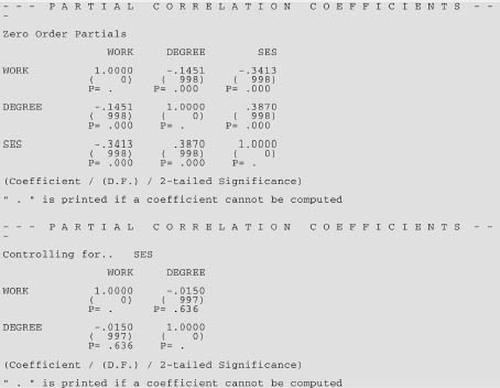
Using SPSS software, partial correlations can be calculated straightforwardly. Partial correlations enable the researcher to control for a third variable, i.e. to see the correlation between two variables of interest once the effects of a third variable have been removed, hence rendering more accurate the relationship between the two variables of interest. As Turner (1997: 33) remarks: partialling can rule out special or specific relationships that do not hold true when variables have been controlled. In our example we have socio-economic status, part-time working and class of degree. We may be interested in investigating the effect of part-time working on class of degree, controlling for the effects of socio-economic status. SPSS enables us to do this at the touch of a button, producing output on partial correlations (Figure 35.8).
The SPSS output (Figure 35.8) indicates that in the second of the tables, the correlation coefficients have been controlled for socio-economic status (marked as ‘Controlling for . . SES’). The top row for each variable presents the correlation coefficient; the middle row indicates the numbers of people who responded; and the bottom row presents the level of statistical significance (ρ = 0.000). Here the results indicate that there is a very little partial correlation between part-time working and class of degree (r = –0.0150, degrees of freedom = 997, ρ = 0.636), but that this is not statistically significant, i.e. there is no significant correlation between part-time work and class of degree, when controlled for socio-economic status. However, when we examine the correlation coefficient for socio-economic status, in the first table there was a very different correlation coefficient (r = –0.1451), and this was highly statistically significant (ρ = 0.000). This suggests to us that controlling for socio-economic status has a very considerable effect on the strength of the relationship between the variables ‘part-time work’ and ‘class of degree’. Had the two coefficients here been close then one could have suggested that controlling for socio-economic status had very little effect on the strength of the relationship between the variables ‘part-time work’ and ‘class of degree’.
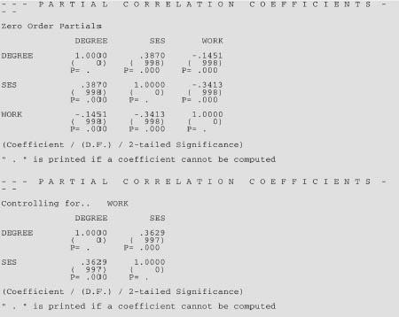
This time let us imagine that we wish to explore the relationship between socio-economic status and class of degree, controlling for part-time working (Figure 35.9). The SPSS output indicates that the correlation coefficients have been controlled for part-time work (marked as ‘Controlling for . . Work’). Here the results indicate that there is a very strong partial correlation between socio-economic status and class of degree (r = 0.3629, degrees of fireedom = 997, ρ = 0.000), i.e. that this is statistically significant. When we examine the correlation coefficient for socio-economic status, in the first table we see that the correlation coefficient (r = 0.3870) is very similar to the correlation coefficient found when the variable ‘part-time work’ has been controlled (the coefficient before being controlled being 0.3870 and the coefficient after being controlled being 0.3629). This suggests that controlling for part-time work status has very little effect on the strength of the relationship between the variables ‘socio-economic status’ and ‘class of degree’. Partial correlation enables relationships to be calculated after controlling for one or more variables.
We need to know how reliable is our instrument for data collection. Reliability in quantitative analysis takes two main forms, both of which are measures of internal consistency: the split-half technique and the alpha coefficient. Both calculate a coefficient of reliability that can lie between 0 and 1. The formula for calculating the Spearman-Brown split-half reliability (discussed in Chapter 10) is:

where r = the actual correlation between the halves of the instrument (this requires the instrument to be able to be divided into two matched halves in terms of content and difficulty). So, for example, if the correlation coefficient between the two halves is 0.85 then the formula would be worked out thus:
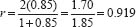
Hence the split-half reliability coefficient is 0.919, which is very high. SPSS automatically calculates split-half reliability at the click of a button.
An alternative calculation of reliability as internal consistency can be found in Cronbach’s alpha, frequently referred to simply as the alpha coefficient of reliability. The Cronbach alpha provides a coefficient of inter-item correlations. What it does is to calculate the average of all possible split-half reliability coeffi-cients. It is a measure of the internal consistency amongst the items (not, for example, the people) and is used for multi-item scales. SPSS calculates Cronbach’s alpha at the click of a button, the formula for alpha is:

where n = the number of items in the test or survey (e.g. questionnaire) and rii = the average of all the inter-item correlations. Let us imagine that the number of items in the survey is ten, and that the average correlation is 0.738. The alpha correlation can be calculated thus:
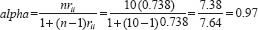
This yields an alpha coefficient of 0.97, which is very high. For the split-half coefficient and the alpha coeffi-cient the following guidelines can be used:
>0.90 very highly reliable
0.80–0.90 highly reliable
0.70–0.79 reliable
0.60–0.69 marginally/minimally reliable
<0.60 unacceptably low reliability.
Bryman and Cramer (1990: 71) suggest that the reliability level is acceptable at 0.8, though others suggest that it is acceptable if it is 0.67 or above.
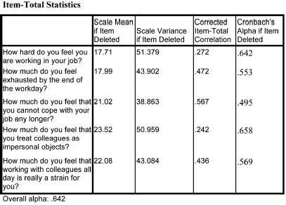
If the researcher is using SPSS then there is a function that enables items to be discovered that might be exerting a negative influence on the Cronbach alpha. Table 35.16 provides an example of this, which indicates in the final column what the Cronbach alpha would be if any of the items were to be removed as unreliable.
In the example, the overall alpha is given as 0.642, but it can be seen that if the item ‘How much do you feel that you treat colleagues as impersonal objects?’ were removed, then the overall reliability would rise to 0.658. The researcher, then, may wish to remove that item – this is particularly true where the researcher is conducting a pilot to see which items are reliable and which are not.
 Companion Website
 The companion website to the book includes PowerPoint slides for this chapter, which list the structure of the chapter and then provide a summary of the key points in each of its sections. This resource can be found online at www.routledge.com/textbooks/cohen7e.
Additionally readers are recommended to access the online resources for Chapter 36 as these contain materials that apply to the present chapter, such as the SPSS Manual which guides readers through the SPSS commands required to run statistics in SPSS, together with data files of different data sets.