measures of difference between groups
Inferential statistics |
CHAPTER 36 |
The previous chapter introduced descriptive statistics. This chapter moves to inferential statistics, those statistics that enable researchers to make inferences about the wider population (discussed in Chapter 34). Here we introduce difference tests, regression and multiple regression, and, arising from both difference testing and regression analysis, the need for standardized scores, and how they can be calculated. The chapter covers:
measures of difference between groups
the t-test (a test of difference for parametric data)
analysis of variance (a test of difference for parametric data)
the chi-square test (a test of difference and a test of goodness of fit for non-parametric data)
degrees of freedom (a statistic that is used in calculating statistical significance in considering difference tests)
the Mann-Whitney and Wilcoxon tests (tests of difference for non-parametric data)
the Kruskal-Wallis and Friedman tests (tests of difference for non-parametric data)
regression analysis (prediction tests for parametric data)
simple linear regression (predicting the value of one variable from the known value of another variable)
multiple regression (calculating the different weightings of independent variables on a dependent variable)
standardized scores (used in calculating regressions and comparing sets of data with different means and standard deviations)
Both separately and together, these statistics constitute powerful tools in the arsenal of statistics for analysing numerical data. We give several worked examples for clarification, and take the novice reader by the hand through these.
Researchers will sometimes be interested to find whether there are differences between two or more groups of subsamples, answering questions such as: ‘Is there a significant difference between the amount of homework done by boys and girls?’ ‘Is there a significant difference between test scores from four similarly mixed-ability classes studying the same syllabus?’ ‘Does school A differ significantly from school B in the stress level of its sixth form students?’ Such questions require measures of difference. This section introduces measures of difference and how to calculate difference. The process commences with the null hypothesis, stating that ‘there is no statistically significant difference between the two groups’, or ‘there is no statistically significant difference between the four groups’, and, if this is not supported, then the alternative hypothesis is supported, namely ‘there is a statistically significant difference between the two (or more) groups’. We discuss difference tests for parametric and non-parametric data.
Before going very far one has to ascertain:
a the kind of data with which one is working, as this affects the choice of statistic used;
b the number of groups being compared, to discover whether there is a difference between them. Statistics are usually divided into those which measure differences between two groups and those which measure differences between more than two groups;
c whether the groups are related or independent. Independent groups are entirely unrelated to each other, e.g. males and females completing an examination; related groups might be the same group voting on two or more variables or the same group voting at two different points in time (e.g. a pre-test and a post-test).
Decisions on these matters will affect the choice of statistics used. Our discussion will proceed thus: first (in section 36.2) we look at a simple difference test for two groups using parametric data, which is the t-test; second (36.3) we look at differences between three or more groups using parametric data (analysis of variance (ANOVA) with a post hoc test (the Tukey test)); third (36.4) we look at a test of difference for categorical data (the chi-square test). Then, fourth (36.5), we introduce the ‘degrees of freedom’. Fifth (36.6) we look at differences between two groups using non-parametric data (the Mann-Whitney and Wilcoxon tests); sixth (36.7) we look at differences between three or more groups using non-parametric data (the Kruskal-Wallis and the Friedman tests). Seventh (36.8) we move from difference testing to prediction, using regression analysis. Eighth (36.11), as regression analysis often uses standardized scores, we introduce standardized scores. As in previous examples, we will be using SPSS to illustrate our points.
The t-test is used to discover whether there are statistically significant differences between the means of two groups, using parametric data drawn from random samples with a normal distribution. It is used to compare the means of two groups randomly assigned, for example on a pre-test and a post-test in an experiment.
The t-test has two variants: the t-test for independent samples and the t-test for related (or ‘paired’) samples. The former assumes that the two groups are unrelated to each other; the latter assumes that it is the same group either voting on two variables or voting at two different points in time about the same variable. We will address the former of these first. The t-test assumes that one variable is categorical (e.g. males and females) and one is a continuous variable (e.g. marks on a test). The formula used calculates a statistic based on:
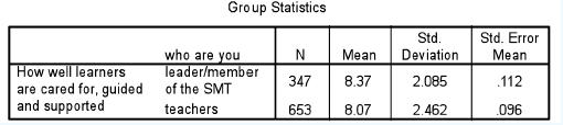
Let us imagine that we wish to discover whether there is a statistically significant difference between the leader/senior management team (SMT) of a group of randomly chosen schools and the teachers, concerning how well learners are cared for, guided and supported. The data are ratio, the participants having had to award a mark out of ten for their response, the higher the mark the greater is the care, guidance and support offered to the students. The t-test for two independent samples presents us with two tables in SPSS. First it provides the average (mean) of the voting for each group: 8.37 for the leaders/senior managers and 8.07 for the teachers, i.e. there is a difference of means between the two groups. Is this difference statistically significant, i.e. is the null hypothesis (‘there is no statistically significant difference between the leaders/SMT and the teachers’) supported or not supported? We commence with the null hypothesis (‘there is no statistically significant difference between the two means’) and then we set the level of significance (a) to use for supporting or not supporting the null hypotheses; for example we could say ‘Let α=0.05’. Then the data are computed as in Table 36.1.
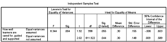
In running the t-test SPSS gives us back what, at first glance, seems to be a morass of information. Much of this is superfluous for our purposes here. We will concern ourselves with the most important pieces of data for introductory purposes here: the Levene test and the significance level for a two-tailed test (Sig. 2-tailed) (Table 36.2).
The Levene test is a guide as to which row of the two to use (‘equal variances assumed’ and ‘equal variances not assumed’). Look at the column ‘Sig.’ in the Levene test (0.004). If the probability value is statistically significant (as in this case (0.004)) then variances are unequal and the researcher needs to use the second row of data (‘Equal variances not assumed’); if the probability value is not significant (ρ>0.05) then equal variances are assumed and s/he uses the first row of data (‘Equal variances assumed’). Once s/he has decided which row to use then the Levene test has served its purpose and s/he can move on. For our commentary here the purpose of the Levene test is only there to determine which row to look at of the two presented.
Having discovered which row to follow, in our example it is the second row, we go along to the column ‘Sig. (2-tailed)’. This tells us that there is a statistically significant difference between the two groups –leaders/SMT and the teachers –because the significance level is 0.044 (i.e. ρ<0.05). Hence we can say that the null hypothesis is not supported, that there is a statistically significant difference between the means of the two groups (ρ = 0.044), and that the mean of the leaders/SMT is statistically significantly higher (8.37) than the mean of the teachers (8.07), i.e. the leaders/SMT of the schools think more highly than the teachers in the schools that the learners are well cared for, guided and supported.
Look at Table 36.2 again, and at the column ‘Sig. (2-tailed)’. Had equal variances been assumed (i.e. if the Levene test had indicated that we should remain on the top row of data rather than the second row of data) then we would not have found a statistically significant difference between the two means (ρ=0.055, i.e. ρ>0.05). Hence it is sometimes important to know whether equal variances are to be assumed or not to be assumed.
In the example here we find that there is a statistically significant difference between the means of the two groups, i.e. the leaders/SMT do not share the same perception as the teachers that the learners are well cared for, guided and supported, typically the leaders/SMT are more generous than the teachers. This is of research interest, e.g. to discover the reasons for, and impact of, the differences of perception. It could be, for example, that the leaders/SMT have a much rosier picture of the situation than the teachers, and that the teachers –the ones who have to work with the students on a close daily basis –are more in touch with the students and know that there are problems, a matter to which the senior managers may be turning a blind eye.
In reporting the t-test here the following form of words can be used:
The mean score of the leaders/SMT on the variable ‘How well learners are cared for, guided and supported’ (M = 8.37, SD = 2.085) is statistically significantly higher (t=2.02, df=811.922), two-tailed (ρ = 0.044) than those of teachers on the same variable (M = 8.07, SD = 2.462).
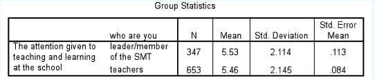
Let us take a second example. Here the leaders/SMT and teachers are voting on ‘the attention given to teaching and learning at the school’, again awarding a mark out of ten, i.e. ratio data. The mean for the leaders/SMT is 5.53 and for the teachers it is 5.46. Are these means statistically significantly different (Tables 36.3 and 36.4)?
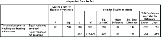
If we examine the Levene test (Sig.) we find that equal variances are assumed (ρ = 0.728), i.e. we remain on the top row of the data output. Running along to the column headed ‘Sig. (2-tailed)’ we find that ρ = 0.610, i.e. there is no statistically significant difference between the means of the two groups, therefore the null hypothesis (there is no statistically significant difference between the means of the two groups) is supported. This should not dismay the researcher; finding or not finding a statistically significant difference is of equal value in research –a win-win situation. Here, for example, one can say that there is a shared perception between the leaders/managers and the teachers on the attention given to teaching and learning in the school, even though it is that the attention given is poor (means of 5.53 and 5.46 respectively). The fact that there is a shared perception – that both parties see the same problem in the same way – offers a positive prospect for development and a shared vision, i.e. even though the picture is poor, nevertheless it is perhaps more positive than if there were very widely different perceptions.
In reporting the t-test here the following form of words can be used:
The mean score for the leaders/SMT on the variable ‘The attention given to teaching and learning at the school’ (M = 5.53, SD = 2.114) did not differ statistically significantly (t = 0.510, df=998, two-tailed ρ = 0.610) from that of the teachers (M = 5.46, SD = 2.145).
The t-test for independent examples is a very widely used statistic, and we support its correct use very strongly.
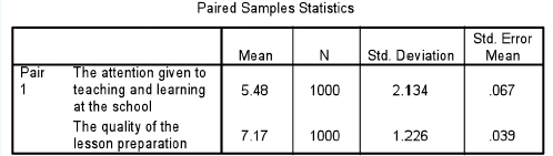
Less frequently used is the t-test for a paired (related) sample, i.e. where the same group votes on two variables (e.g. liking for mathematics and music), or the same sample group is measured on two occasions (e.g. the pre-test and the post-test) or under two conditions, or the same variable is measured at two points in time. In Table 36.5 two variables are paired, with marks awarded by the same group.
One can see here that we are looking to see if the mean of the 1,000 respondents who voted on ‘the attention given to teaching and learning at the school’ (mean=5.48) is statistically significantly different from the mean of the same group voting on the variable ‘the quality of the lesson preparation’ (mean=7.17) using Table 36.6.
Here we can move directly to the final column (‘Sig. (2-tailed)’) where we find that ρ = 0.000, i.e. ρ<0.00L telling us that the null hypothesis is not supported, and that there is a statistically significant difference between the two means, even though it is the same group that is awarding the marks.
The issue of testing the difference between two proportions is set out on the accompanying website.
To replace statistical significance in difference measurement, calculating effect size can be conducted using ‘partial eta squared’ and Cohen’s d. (In SPSS the command sequence is: Analyze → General Linear Model → Univariate → Estimates of effect size.) Eta squared is the proportion of the total variance that can be attributed to a particular effect, whilst partial eta squared is the proportion of the effect plus error variance that can be attributed to a particular effect. Partial eta squared and Cohen’s d are the preferred measures here.
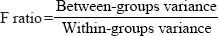
The t-test is useful for examining differences between two groups of respondents, or the same group on either two variables or two occasions, using parametric data from a random sample and assuming that each datum value is independent of the others. However, in much educational research we may wish to investigate differences between more than two groups. For example we may wish to look at the examination results of four regions or four kinds of schools. In this case the t-test will not suit out purposes, and we must turn to analysis of variance. Analysis of variance (ANOVA) is premised on the same assumptions as t-tests, namely random sampling, a normal distribution of scores and parametric data, and it can be used with three or more groups. There are several kinds of analysis of variance; here we introduce only the two most widely used versions: the one-way analysis of variance and the two-way analysis of variance. Analysis of variance, like the t-test, assumes that the independent variable(s) is/are categorical (e.g. teachers, students, parents, governors) and one is a continuous variable (e.g. marks on a test). It calculates the F ratio, given as:
ANOVA calculates the means for all the groups, then it calculates the average of these means. For each group separately it calculates the total deviation of each individual’s score from the mean of the group (within-groups variation). Finally it calculates the deviation of each group mean from the grand mean (between-groups variation).
Let us imagine that we have four types of school:
rural primary
rural secondary
urban primary
urban secondary.
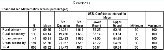
Let us imagine further that all the schools in these categories have taken the same standardized test of mathematics, and the results have been given as a percentage, as shown in Table 36.7. This gives us the means, standard deviations, standard error, confidence intervals, and the minimum and maximum marks for each group. At this stage we are only interested in the means:
rural primary: |
mean= 59.85% |
rural secondary: |
mean=60.44% |
urban primary: |
mean=50.64% |
urban secondary : |
mean = 51.70% |
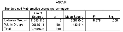
Are these means statistically significantly different? Analysis of variance (ANOVA) will tell us whether they are. We commence with the null hypothesis (‘there is no statistically significant difference between the four means’) and then we set the level of significance (α) to use for supporting or not supporting the null hypothesis; for example we could say ‘Let α=0.05’. Table 36.8 shows the SPSS calculations.
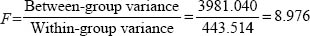
This tells us that, for three degrees of freedom (df), the F-ratio is 8.976. The F-ratio is the between-group mean square (variance) divided by the within-group mean square (variance), i.e.
By looking at the final column (‘Sig.’) ANOVA tell us that there is a statistically significant difference between the means (ρ = 0.000). This does not mean that all the means are statistically significantly different from each other, but that some are. For example, it may be that the means for the rural primary and rural secondary schools (59.85% and 60.44% respectively) are not statistically significantly different, and that the means for the urban primary schools and urban secondary schools (50.64% and 51.70% respectively) are not statistically significantly different. However it could be that there is a statistically significant difference between the scores of the rural (primary and secondary) and the urban (primary and secondary) schools. How can we find out which groups are different from each other? The purpose of a post hoc test is to find out exactly where those differences are.
There are several tests that can be employed here, though we will only concern ourselves with a very commonly used test: the Tukey honestly significant difference test, sometimes called the ‘Tukey hsd’ test, or simply (as in SPSS) the Tukey test. Others include the Bonferroni and Scheffé test; they are more rigorous than the Tukey test and tend to be used less frequently. The Scheffé test is very similar to the Tukey hsd test, but it is more stringent that the Tukey test in respect of reducing the risk of a Type I error, though this comes with some loss of power: one may be less likely to find a difference between groups in the Scheffé test. The Tukey test groups together subsamples whose means are not statistically significantly different from each other and places them in a different group from a group whose means are statistically significantly different from the first group. Let us see what this means in our example of the mathematics results of four types of school.
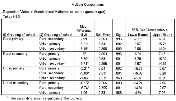
Table 36.9 takes each type of school and compares it with the other three types, in order to see where there may be statistically significant differences between them. Here the rural primary school is first compared with the rural secondary school (row one of the left-hand column cell named ‘Rural primary’), and no statistically significant difference is found between them (Sig. =0.996, i.e. ρ>0.05). The rural primary school is then compared with the urban primary school and a statistically significant difference is found between them (Sig. =0.002, i.e. ρ<0.05). The rural primary school is then compared with the urban secondary school, and, again, a statistically significant difference is found between them (Sig. =0.003, i.e. ρ<0.05). The next cell of the left-hand column commences with the rural secondary school, and this is compared with the rural primary school, and no statistically significant difference is found (Sig. =0.996, i.e. ρ>0.05). The rural secondary school is then compared to the urban primary school and a statistically significant difference is found between them (Sig. =0.001, i.e. ρ<0.05). The rural secondary school is then compared with the urban secondary school, and, again, a statistically significant difference is found between them (Sig. =0.001, i.e. ρ<0.05). The analysis is continued for the urban primary and the urban secondary school. One can see that the two types of rural school do not differ statistically significantly from each other, that the two types of urban school do not differ statistically significantly from each other, but that the rural and urban schools do differ statistically significantly from each other. We can see where the null hypothesis is supported and where it is not supported.
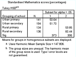
In fact the Tukey test in SPSS presents this very clearly, as shown in Table 36.10. Here one group of similar means (i.e. those not statistically significantly different from each other: the urban primary and urban secondary) is placed together (the column labelled ‘1’) and the other group of similar means (i.e. those not statistically significantly different from each other: the rural primary and rural secondary) is placed together (the column labelled ‘2’). SPSS automatically groups these and places them in ascending order (the group with the lowest means appears in the first column, and the group with the highest means is in the second column). So, one can see clearly that the difference between the schools lies not in the fact that some are primary and some are secondary, but that some are rural and some are urban, i.e. the differences relate to geographical location rather than age group in the school. The Tukey test helps us to locate exactly where the similarities and differences between groups lie. It places the means into homogeneous subgroups, so that we can see which means are close together but different from other groups of means.
Analysis of variance here tells us that there are or are not statistically significant differences between groups; the Tukey test indicates where these differences lie, if they exist. We advise using the two tests together. Of course, as with the t-test, it is sometimes equally important if we do not find a difference between groups as if we do find a difference. For example, if we were to find that there was no difference between four groups (parents, teachers, students and school governors/leaders) on a particular issue, say the move towards increased science teaching, then this would give us greater grounds for thinking that a proposed innovation – the introduction of increased science teaching – would stand a greater chance of success than if there had been statistically significant differences between the groups. Finding no difference can be as important as finding a difference.
In reporting analysis of variance and the Tukey test one could use a form of words thus:
Analysis of variance found that there was a statistically significant difference between rural and urban schools (F14 = 8.975, ρ<0.001). The Tukey test found that the means for rural primary schools and rural secondary schools (59.85 and 60.44 respectively) were not statistically significantly different from each other, and that the means for urban primary schools and urban secondary schools (50.64 and 51.70 respectively) were not statistically significantly different from each other. The homogeneous subsets calculated by the Tukey test reveal two subsets in respect of the variable ‘Standardized mathematics scores’: (a) urban primary and urban secondary schools; (b) rural primary and rural secondary scores. The two subsets reveal that these two groups were distinctly and statistically significantly different from each other in respect of this variable. The means of the rural schools were statistically significantly higher than the means of the urban schools.
For repeated measures in ANOVA (i.e. the same groups under three or more conditions), with the Tukey test and a measure of effect size, the SPSS command sequence is: Analyze → General Linear Model → Repeated Measures → In the box ‘Within-Subject Factor Name’ name a new variable → In the box ‘Number of Levels’ insert the number of dependent variables that you wish to include → Click on ‘Add’ → Click on ‘Define’ → Send over the dependent variables that you wish to include (the number of variables must be the same as the ‘Number of Levels’) into the box ‘Within-Subjects Variables’ → Send over the independent variable into the box ‘Between-Subjects Factors’ → Click on ‘Options’ → Click on ‘Estimates of effect size’ → Click on ‘Continue’ → Click ‘Post Hoc’ → Send over the factor from the ‘Factor(s)’ box to the ‘Post Hoc Tests for’ box → Click on ‘Tukey’ → Click ‘Continue’ (which returns you to the original screen) → Click ‘OK’. This will give you several boxes in the output. Go to ‘Multivariate Tests’; the furthest right-hand column has the partial eta squared. Go to the row that contains the last box, and look at the partial eta squared (e.g. ‘Pillai’s Trace’ and Wilks’s Lamda’); this gives the partial eta squared.
The example of ANOVA above illustrates one-way analysis of variance, i.e. the difference between the means of three or more groups on a single independent variable. Additionally ANOVA can take account of more than one independent variable. Two-way analysis of variance is used ‘to estimate the effect of two independent variables (factors) on a single variable’ (Cohen and Holliday, 1996: 277). Let us take the example of how examination performance in science is affected by both age group and sex. Two-way ANOVA enables the researcher not only to examine the effect of each independent variable but also the interaction effects on each other of the two independent variables, i.e. how sex effects are influenced or modified when combined with age group effects. We may discover, for example, that age group has a differential effect on examination performance according to whether one is male or female, i.e. there is an interaction effect.
For two-way analysis of variance the researcher requires two independent categorical (nominal) variables (e.g. sex, age group) and one continuous dependent variable (e.g. performance on examinations). Two-way ANOVA enables one to calculate three effects. In the example here they are:
difference in examination performance by sex;
difference in examination performance by age group;
the interaction of sex and age group on examination, e.g. is there a difference in the effects of age group on examination performance for males and females?
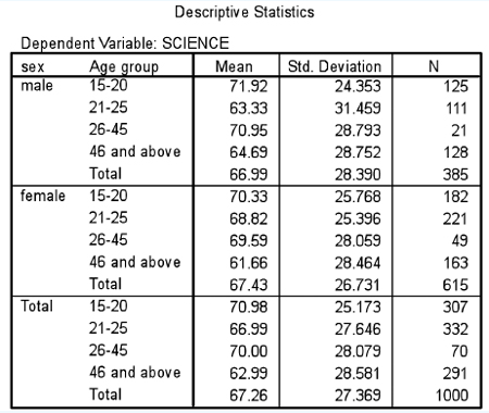
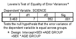
We will use SPSS to provide an example of this. SPSS first presents descriptive statistics, for example Table 36.11. This simply presents the data, with means and standard deviations. Next SPSS calculates the Levene test for equality of error variances, degrees of freedom and significance levels, as shown in Table 36.12.
This test enables the researcher to know whether there is equality across the means. She needs to see if the significance level is greater than 0.05. The researcher is looking for a significance level greater than 0.05, i.e. not statistically significant, which supports the null hypothesis that holds that there is no statistically significant difference between the means and variances across the groups (i.e. to support the assumptions of ANOVA). In our example this is not the case as the significance level is 0.001. This means that she has to proceed with caution as equality of variances cannot be assumed. SPSS provides her with important information, as shown in Table 36.13.
TABLE 36.12 THE LEVENE TEST OF EQUALITY OF VARIANCES IN A TWO-WAY ANALYSIS OF VARIANCE (SPSS OUTPUT)
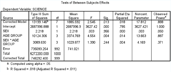
Here one can see the three sets of independent variables listed (SEX, AGE GROUP, SEX*AGE GROUP). The column headed ‘Sig.’ shows that the significance levels for the three sets are, respectively: 0.956, 0.004 and 0.244. Hence one can see that sex does not have a statistically significant effect on science examination performance. Age group does have a statistically significant effect on the performance in the science examination (ρ=0.004). The interaction effect of sex and age group does not have a statistically significant effect on performance, i.e. there is no difference in the effect on science performance for males and females (ρ=0.244). SPSS also computes the effect size (Partial Eta squared). For the important variable AGE GROUP this is given as 0.014, which shows that the effect size is very small indeed, suggesting that, even though statistical significance has been found, the actual difference in the mean values is very small.
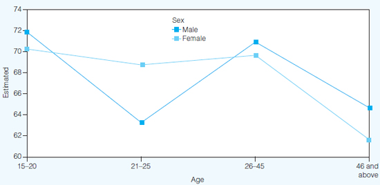
As with one-way ANOVA, the Tukey test can be applied here to present the homogeneous groupings of the subsample means. SPSS can also present a graphic plot of the two sets of scores, which gives the researcher a ready understanding of the effects of the males and females across the four age groups in their science examination, as shown in Figure 36.1.
In reporting the results of the two-way analysis of variance one can use the following form of words:
A two-way between-groups analysis of variance was conducted to discover the impact of sex and age group on performance in a science examination. Subjects were divided into four groups by age: Group 1: 15–20 years; Group 2: 21–25 years; Group 3: 26–5 years; and Group 4: 46 years and above. There was a statistically significant main effect for age group (F=4.554, ρ=0.004), however the effect size was small (partial eta squared=0.014). The main effect for sex (F = 0.003, ρ=0.956) and the interaction effect (F= 1.390, ρ=0.244) were not statistically significant.
To run two-way ANOVA in SPSS the command sequence is: ‘Analyze’ → Click on ‘General Linear Model’ → Click on ‘Univariate’ → Send the dependent variable to the box ‘Dependent Variable’ → Send the independent variables to the box ‘Fixed Factors’ → Click on the ‘Options’ box; in the ‘Display’ area, check the boxes ‘Descriptive Statistics’ and ‘Estimates of effect size’ → Click ‘Continue’ → Click on the ‘Post Hoc’ box, and send over from the ‘Factors’ box to the ‘Post Hoc tests for’ box those factors that you wish to investigate in the post hoc tests → Click the post hoc test that you wish to use (e.g. ‘Tukey’) → Click ‘Continue’ → Click the ‘Plots’ box → Move to the ‘Horizontal’ box the factor that has the most groups → Move to the ‘Separate lines’ box the factor the other independent variable → Click on ‘Add’ → Click on ‘Continue’ → Click on ‘OK’.
Estimated marginal means of science
FIGURE 36.1 Graphic plots of two sets of scores on a dependent variable
Multiple analysis of variance (MANOVA) is designed to see the effects of one categorical independent variable on two or more continuous variables (e.g. ‘do males score more highly than females in terms of how hard they work and their IQ’).
To run MANOVA, the SPSS command sequence is: ‘Analyze’ → Click on ‘General Linear Model’ → Click on ‘Multivariate’ → Send to the box ‘Dependent Variables’ the dependent variables that you wish to include → Send to the ‘Fixed Factors’ box the independent variable that you wish to use → Click on ‘Model’ and ensure that the ‘Full factorial’ (in the ‘Specify Model’ box) and the ‘Type III’ (in the ‘Sum of Squares’) boxes are selected → Click on ‘Continue’ → Click on the ‘Options’ box and send to the ‘Display Means for’ box the independent variable that you wish to include → In the ‘Display’ section, click on ‘Descriptive Statistics’, ‘Estimates of effect size’ and ‘Homogeneity tests’ → Click on ‘Continue’ → If you want a post hoc test click on ‘Post Hoc’ → Send over the independent variable from the ‘Factor(s)’ box to the ‘Post Hoc tests for’ box (if you want a post hoc test and if your independent variable has three or more values) → Click on ‘Tukey’ → Click on ‘Continue’ → Click on ‘OK’.
The standard text on one-way and two-way analysis of variance (ANOVA) and multiple analysis of variance (MANOVA) is Tabachnick and Fidell (2007), and we refer readers to this text. For further guidance on running SPSS for these matters and interpreting the SPSS output, we refer readers to Pallant (2007).
Difference testing is an important feature in understanding data. We can conduct a statistical test to investigate difference; it is the chi-square test (Χ2) (pronounced ‘kigh’, as in ‘high’). The chi-square test is a test of difference that can be conducted for a univariate analysis (one categorical variable), and between two categorical variables. The chi-square test measures the difference between a statistically generated expected result and an actual (observed) result to see if there is a statistically significant difference between them, i.e. to see if the frequencies observed are significant; it is a measure of ‘goodness of fit’ between an expected and an actual, observed result or set of results. The expected result is based on a statistical process discussed below. The chi-square statistic addresses the notion of statistical significance, itself based on notions of probability. Here is not the place to go into the mathematics of the test, not least because computer packages automatically calculate the results. That said, the formula for calculating chi-square is:

where
O= observed frequencies
E=expected frequencies
entity=the sum of
For univariate data let us take the example of 120 students who were asked which of four teachers they preferred. We start with the null hypothesis that states that there is no difference in the preferences for four teachers, i.e. that the 120 scores are spread evenly across the four teachers, thus:
Frequencies |
Teacher |
Teacher |
Teacher |
Teacher |
|
A |
B |
C |
D |
Observed |
20 |
70 |
10 |
20 |
Expected |
30 |
30 |
30 |
30 |
Residual (difference between observed and expected frequencies) |
–10 |
40 |
–20 |
–10 |
Using the formula above we compute the chi-square figure thus:
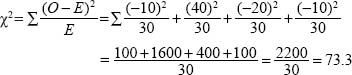
The chi-square value here is 73.3, with three degrees of freedom (explained below). In a table of critical values for chi-square distributions (usually in the appendices of most statistics books and freely available on the internet) we look up the level of statistical significance for three degrees of freedom:
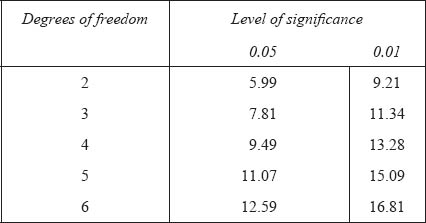
We find that, at 73.3, the chi-square value is considerably larger than 11.34, i.e. it has a probability level stronger than 0.01, i.e. of 0.000, i.e. there is a statistically significant difference between the observed and expected frequencies, i.e. not all teachers are equally preferred (more people preferred Teacher B, and this was statistically significant).
If all the teachers were equally popular then the observed frequencies would not differ much from the expected frequencies. However, if the observed frequencies differ a lot from the expected frequencies, then it is likely that all teachers are not equally preferred, and this is what was found here.
For bivariate data a similar procedure can be followed. Here the chi-square test is a test of independence, to see whether there is a relationship or association between two categorical variables. Let us say that we have a crosstabulation of males and females and their liking for maths (like/dislike). We start with the null hypothesis that states that there is no statistically significant difference between the males and females (variable 1) in their (dis)liking for mathematics (variable 2), and the onus on the data is not to support this. We then set the level of significance (a) that we wish to use for supporting or not supporting the null hypothesis; for example we could say ‘Let α=0.05’. Having found out the true voting we set out a 2 X 2 crosstabulation thus, with the observed frequencies in the cells:
|
Male |
Female |
Total |
Like mathematics |
60 |
25 |
85 |
Dislike mathematics |
35 |
75 |
110 |
Total |
95 |
100 |
195 |
These are the observed frequencies. To find out the expected frequencies for each cell we use the formula:
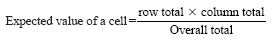
Hence we can calculate the expected frequencies for each thus (figures rounded):
|
Male |
Female |
Total |
Like |
(85 x 95)/ |
(85 x 100)/ |
85 |
mathematics |
195 = 41.4 |
195 = 43.6 |
|
Dislike |
(110x95)/ |
(110 x 100)/ |
110 |
mathematics |
195 = 53.6 |
195 = 56.4 |
|
Total |
95 |
100 |
195 |
The chi-square value, using the formula above is:
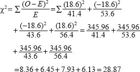
When we look up the chi-square value of 28.87 in the tables of the critical values of the chi-square distribution, with two degrees of freedom we observe that the figure of 28.87 is larger than the figure of 9.21 required for statistical significance at the 0.01 level. Hence we conclude that the distribution of likes and dislikes for mathematics by males and females is not simply by chance but that there is a real, statistically significant difference between the voting of males and females here. Hence the null hypothesis is not supported and the alternative hypothesis, that there is a statistically significant difference between the voting of the two groups, is supported.
We do not need to perform these calculations by hand. Computer software such as SPSS will do all the calculations at the press of a button.
We recall that the conventionally accepted minimum level of significance is usually 0.05, and we used this level in the example; the significance level of our data here is smaller than either the 0.05 and 0.01 levels, i.e. it is highly statistically significant.
One can report the results of the chi-square test thus, for example:
When the chi-square statistic was calculated for the distribution of males and females on their liking for mathematics, a statistically significant difference was found between the males and the females (Χ2=28.87, d.f=2, ρ =0.000).
We use Yates’s correction (a continuity correction) to compensate for the overestimate of the chi-square in a 2 X 2 table, and this can be activated by a single button in SPSS or other software.
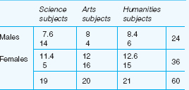
The chi-square statistic is normally used with nominal (categorical) data, and our example in Table 36.14 illustrates this. This is a further example of the chi-square statistic, with data that are set into a contingency table, this time in a 2 X 3 contingency table, i.e. two horizontal rows and three columns (contingency tables may contain more than this number of variables). The example in Table 36.14 presents data concerning 60 students’ entry into science, arts and humanities, in a college, and whether the students are male or female (Morrison, 1993: 132–4). The lower of the two figures in each cell is the number of actual students who have opted for the particular subjects (sciences, arts, humanities). The upper of the two figures in each cell is what might be expected purely by chance to be the number of students opting for each of the particular subjects. The figure is arrived at by statistical computation, hence the decimal fractions for the figures. What is of interest to the researcher is whether the actual distribution of subject choice by males and females differs significantly from that which could occur by chance variation in the population of college entrants.
The researcher begins with the null hypothesis that there is no statistically significant difference between the actual results noted and what might be expected to occur by chance in the wider population. When the chi-square statistic is calculated, if the observed, actual distribution differs from that which might be expected to occur by chance alone, then the researcher has to determine whether that difference is statistically significant, i.e. not to support the null hypothesis.
In our example of 60 students’ choices, the chi-square formula yields a final chi-square value of 14.64. This we refer to the tables of the critical values of the chi-square distribution (an extract from which is set out for the first example above) to determine whether the derived chi-square values indicate a statistically significant difference from that occurring by chance.
The researcher will see that the ‘degrees of freedom’ (a mathematical construct that is related to the number of restrictions that have been placed on the data) have to be identified. In many cases, to establish the degrees of freedom, one simply takes 1 away from the total number of rows of the contingency table and 1 away from the total number of columns and adds them; in this case it is (2–1)+(3–1)=3 degrees of freedom. Degrees of freedom are discussed in the next section. (Other formulae for ascertaining degrees of freedom hold that the number is the total number of cells minus one.) The researcher looks along the table from the entry for the three degrees of freedom and notes that the derived chi-square value calculated (14.64) is statistically significant at the 0.01 level, i.e. is higher than the required 11.34, indicating that the results obtained –the distributions of the actual data – could not have occurred simply by chance. The null hypothesis is not supported, at the 0.01 level of significance. Interpreting the specific numbers of the contingency table (Table 36.14) in educational rather than statistical terms, noting (a) the low incidence of females in the science subjects and the high incidence of females in the arts and humanities subjects, and (b) the high incidence of males in the science subjects and low incidence of males in the arts and humanities, the researcher would say that this distribution is statistically significant – suggesting, perhaps, that the college needs to consider action possibly to encourage females into science subjects and males into arts and humanities.
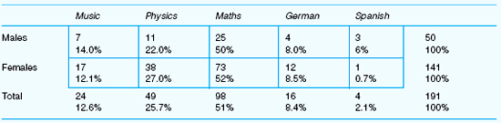
The chi-square test is one of the most widely used tests, and is applicable to nominal data in particular. More powerful tests are available for ordinal, interval and ratio data, and we discuss these separately. However, one has to be cautious of the limitations of the chi-square test. Look at the following example in Table 36.15.
If one were to perform the chi-square test on this table then one would have to be extremely cautious. The chi-square statistic assumes that no more than 20 per cent of the total number of cells contain fewer than five cases. In the example here we have one cell with four cases, another with three, and another with only one case, i.e. three cells out of the ten (two rows – males and females – with five cells in each for each of the rating categories). This means that 30 per cent of the cells contain less than five cases; even though a computer will calculate a chi-square statistic, it means that the result is unreliable. This highlights the point made in Chapter 8 about sampling, namely that the subsample size has to be large. For example, if each category here were to contain five cases then it would mean that the minimum sample size would be 50 (10 X 5), assuming that the data are evenly spread. In the example here, even though the sample size is much larger (191) it still does not guarantee that the 20 per cent rule will be observed, as the data are unevenly spread. When calculating the chi-square statistic, the researcher can use the Fisher Exact Probability Test if more than 25 per cent of the cells have fewer than five cases, and this is automatically calculated and printed as part of the normal output in the chi-square calculation in SPSS.
Because of the need to ensure that at least 80 per cent of the cells of a chi-square contingency table contain more than five cases if confidence is to be placed in the results, it may not be feasible to calculate the chi-square statistic if only a small sample is being used. Hence the researcher would tend to use this statistic for larger-scale survey data. Other tests could be used if the problem of low cell frequencies obtains, e.g. the binomial test and, more widely used, the Fisher Exact Probability Test (Cohen and Holliday, 1996: 218–20). The required minimum number of cases in each cell renders the chi-square statistic problematic, and, apart from with nominal data, there are alternative statistics that can be calculated and which overcome this problem (e.g. the Mann-Whitney, Wilcoxon, Kruskal-Wallis and Friedman tests for non-parametric – ordinal – data, and the t–test and analysis of variance test for parametric – interval and ratio – data).
As the use of statistical significance is being increasingly questioned, it is being replaced with measures of effect size (discussed in Chapter 34). Calculations of effect size for categorical tables use two main statistics:
Phi coefficient for 2 X 2 tables (in which Cohen’s d indicates small effect for 0.10, a medium effect for 0.30 and a large effect for 0.50).
Cramer’s V for contingency tables larger than 2 X 2, which takes account of degrees of freedom.
Two significance tests for very small samples are given in the accompanying website.
The chi-square statistic introduces the term degrees of freedom. Gorard (2001b: 233) suggests that ‘the degrees of freedom is the number of scores we need to know before we can calculate the rest’. Cohen and Holliday (1996: 113) explain the term clearly:
Suppose we have to select any five numbers. We have complete freedom of choice as to what the numbers are. So, we have five degrees of freedom. Suppose however we are then told that the five numbers must have a total value of 25. We will have complete freedom of choice to select four numbers but the fifth will be dependent on the other four. Let’s say that the first four numbers we select are 7, 8, 9, and 10, which total 34, then if the total value of the five numbers is to be 25, the fifth number must be –9.
7+8+9 + 10–9=25
A restriction has been placed on one of the observations; only four are free to vary; the fifth has lost its freedom. In our example then d.f. = 4, that is N –1=5–1=4.
Suppose now that we are told to select any five numbers, the first two of which have to total 9, and the total value of all five has to be 25. Our restriction is apparent when we wish the total of the first two numbers to be 9. Another restriction is apparent in the requirement that all five numbers must total 25. In other words we have lost two degrees of freedom in our example. It leaves us with d.f. = 3, that is, N–2 = 5–2 = 3.
For a cross-tabulation (a contingency table), degrees of freedom refer to the freedom with which the researcher is able to assign values to the cells, given fixed marginal totals, usually given as (number of rows – 1)+(number of columns –1). There are many variants of this, and readers will need to consult more detailed texts to explore this issue. We do not dwell on degrees of freedom here, as it is automatically calculated and addressed in subsequent calculations by most statistical software packages such as SPSS.
The non-parametric equivalents of the t-test are the Mann-Whitney U test for two independent samples and the Wilcoxon test for two related samples, both for use with one categorical variable and a minimum of one ordinal variable. These enable us to see, for example, whether there are differences between males and females on a rating scale.
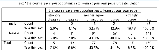
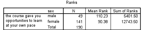
The Mann-Whitney test is based on ranks, ‘comparing the number of times a score from one of the samples is ranked higher than a score from the other sample’ (Bryman and Cramer, 1990: 129) and hence overcomes the problem of low cell frequencies in the chi-square statistic. Let us take an example. Imagine that we have conducted a course evaluation, using five-point rating scales (‘not at all’, ‘very little’, ‘a little’, ‘quite a lot’, ‘a very great deal’), and we wish to find if there is a statistically significant difference between the voting of males and females on the variable ‘The course gave you opportunities to learn at your own pace’. We commence with the null hypothesis (‘there is no statistically significant difference between the two rankings’) and then we set the level of significance (a) to use for supporting or not supporting the null hypothesis; for example we could say ‘Let α=0.05’. A crosstabulation is shown in Table 36.16.
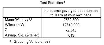
Are the differences between the two groups statistically significant? Using SPSS, the Mann-Whitney statistic is given in Tables 36.17 and 36.18.
Mann-Whitney using ranks (as in Table 36.17) yields a U value of 2,732.500 (as in Table 36.18) from the formula it uses for the calculation (SPSS does this automatically). The important information in Table 36.18 is the ‘Asymp. Sig. (2-tailed)’, i.e. the statistical significance level of any difference found between the two groups (males and females). Here the significance level (ρ=0.019, i.e. ρ<0.05) indicates that the voting by males and females is statistically significantly different and that the null hypothesis is not supported. In the t-test and the Tukey test researchers could immediately find exactly where differences might lie between the groups (by looking at the means and the homogeneous subgroups respectively). Unfortunately the Mann-Whitney test does not enable the researcher to identify clearly where the differences lie between the two groups, so the researcher would need to go back to the crosstabulation to identify where differences lie. In the example above, it appears that the males feel more strongly than the females that the course in question has afforded them the opportunity to learn at their own pace.
In reporting the Mann-Whitney test one could use a form of words such as the following:
When the Mann-Whitney Wallis statistic was calculated to determine whether there was any statistically significant difference in the voting of the two groups (U=2,732.500, ρ =0.019), a statistically significant difference was found between the males and females. A crosstabulation found that males felt more strongly than the females that the course in question had afforded them the opportunity to learn at their own pace.
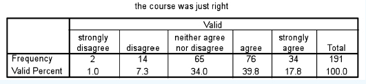
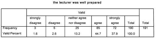
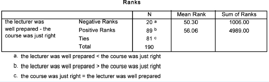
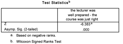
For two related samples (e.g. the same group voting for more than one item, or the same grouping voting at two points in time) the Wilcoxon test is applied, and the data are presented and analysed in the same way as the Mann-Whitney test. For example in Tables 36.19 and 36.20 there are two variables (‘The course was just right’ and ‘The lecturer was well prepared’), voted on by the same group. The frequencies are given. Is there a statistically significant difference in the voting?
As it is the same group voting on two variables, the sample is not independent, hence the Wilcoxon test is used. Using SPSS output, the data analysis shows that the voting of the group on the two variables is statistically significantly different (Tables 36.21 and 36.22).
The reporting of the results of the Wilcoxon test can follow that of the Mann-Whitney test.
For both the Mann-Whitney and Wilcoxon tests, not finding a statistically significant difference between groups can be just as important as finding a statistically significant difference between them, as the former suggests that nominal characteristics of the sample make no statistically significant difference to the voting, i.e. the voting is consistent, regardless of particular features of the sample.
The non-parametric equivalents of analysis of variance are the Kruskal-Wallis test for three or more independent samples and the Friedman test for three or more related samples, both for use with one categorical variable and one ordinal variable. These enable us to see, for example, whether there are differences between three or more groups (e.g. classes, schools, groups of teachers) on a rating scale.
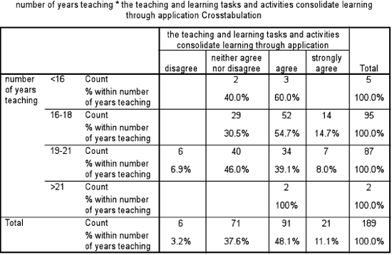
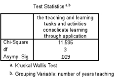
These tests operate in a very similar way to the Mann-Whitney test, being based on rankings. Let us take an example. Teachers in different groups, according to the number of years that they have been teaching, have been asked to evaluate one aspect of a particular course that they have attended (‘The teaching and learning tasks and activities consolidate learning through application’). One of the results is the crosstabulation in Table 36.23. Are the groups of teachers statistically significantly different from each other? We commence with the null hypothesis (‘there is no statistically significant difference between the four groups’) and then we set the level of significance (a) to use for supporting or not supporting the null hypothesis; for example we could say ‘Let α= 0.05’.
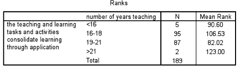
Is the difference in the voting between the four groups statistically significantly different? The Kruskal-Wallis test calculates and presents results in SPSS as shown in Tables 36.24 and 36.25.
The important figure to note here is the 0.009 (‘Asymp. Sig.) – the significance level. Because this is less than 0.05 we can conclude that the null hypothesis (‘there is no statistically significant difference between the voting by the different groups of years in teaching’) is not supported, and that the results vary according to the number of years in teaching of the voters. As with the Mann-Whitney test, the Kruskal-Wallis test tells us only that there is or is not a statistically significant difference, not where the difference lies. To find out where the difference lies, one has to return to the cross-tabulation and examine it. In the example here in Table 36.23 it appears that those teachers in the group which had been teaching from 16–18 years are the most positive about the aspect of the course in question.
In reporting the Kruskal-Wallis test one could use a form of words such as the following:
When the Kruskal-Wallis statistic was calculated to determine whether there was any statistically significant difference in the voting of the four groups (Χ2= 11.595, ρ =0.009), a statistically significant difference was found between the groups which had different years of teaching experience. A crosstabulation found that those teachers in the group that had been teaching from 16–18 years were the most positive about the variable ‘the teaching and learning tasks and activities consolidate learning through application’.
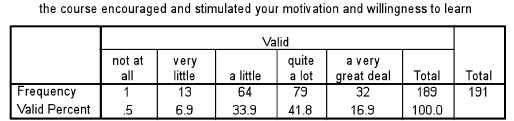
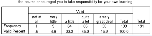
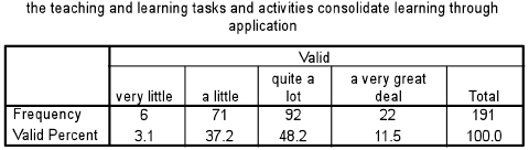
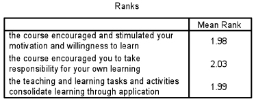
For more than two related samples (e.g. the same group voting for three or more items, or the same grouping voting at three points in time), the Friedman test is applied. For example in Tables 36.26–36.28 are three variables (‘The course encouraged and stimulated your motivation and willingness to learn’; ‘The course encouraged you to take responsibility for your own learning’; and ‘The teaching and learning tasks and activities consolidate learning through application’), all of which are voted on by the same group. The frequencies are given. Is there a statistically significant difference between the groups in their voting?
The Friedman test reports the mean rank and then the significance level; in the examples here the SPSS output has been reproduced in Tables 36.29 and 36.30.
Here one can see that, with a significance level of 0.838 (greater than 0.05), the voting by the same group on the three variables is not statistically significantly different, i.e. the null hypothesis is supported. The reporting of the results of the Friedman test can follow that of the Kruskal-Wallis test.
For both the Kruskal-Wallis and the Friedman tests, as with the Mann-Whitney and Wilcoxon tests, not finding a statistically significant difference between groups can be just as important as finding a statistically significant difference between them, as the former suggests that nominal characteristics of the sample make no statistically significant difference to the voting, i.e. the voting is consistent, regardless of particular features of the sample.
Regression analysis enables the researcher to predict ‘the specific value of one variable when we know or assume values of the other variable(s)’ (Cohen and Holliday, 1996: 88). It is a way of modelling the relationship between variables. We will concern ourselves here with simple linear regression and simple multiple regression, though we will also reference stepwise multiple regression and logistic regression.
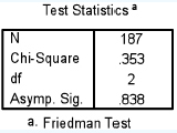
In simple linear regression the model includes one explanatory variable (the independent variable) and one explained variable (the dependent variable). For example, we may wish to see the effect of hours of study on levels of achievement in an examination, to be able to see how much improvement will be made to an examination mark by a given number of hours of study. Hours of study is the independent variable and level of achievement is the dependent variable. Conventionally, as in the example below, one places the independent variable in the vertical axis and the dependent variable in the horizontal axis.
In the example in Figure 36.2 we have taken 50 cases of hours of study and student performance, and have constructed a scatterplot to show the distributions (SPSS performs this function at the click of two or three keys). We have also constructed a line of best fit (SPSS will do this easily) to indicate the relationship between the two variables. The line of best fit is the closest straight line that can be constructed to take account of variance in the scores, and strives to have the same number of cases above it and below it and making each point as close to the line as possible; for example, one can see that some scores are very close to the line and others are some distance away. There is a formula for its calculation, but we do not explore that here.
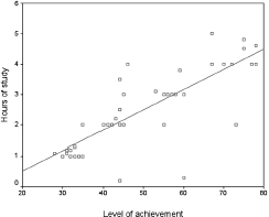
One can observe that the greater the number of hours spent in studying, generally the greater is the level of achievement. This is akin to correlation. The line of best fit indicates not only that there is a positive relationship, but that the relationship is strong (the slope of the line is quite steep). However, where regression departs from correlation is that regression provides an exact prediction of the value – the amount – of one variable when one knows the value of the other. One could read off the level of achievement, for example, if one were to study for two hours (43 marks out of 80) or for four hours (72 marks out of 80), of course, taking no account of variance. To help here scatterplots (e.g. in SPSS) can insert grid lines, for example as shown in Figure 36.3.
It is dangerous to predict outside the limits of the line; simple regression is only to be used to calculate values within the limits of the actual line, and not beyond it. One can observe, also, that though it is possible to construct a straight line of best fit (SPSS does this automatically), some of the data points lie close to the line and some lie a long way from the line; the distance of the data points from the line is termed the residuals, and this would have to be commented on in any analysis (there is a statistical calculation to address this but we do not go into it here).
Where the line strikes the vertical axis is named the intercept. We return to this later, but at this stage we note that the line does not go through the origin but starts a little way up the vertical line. In fact this is all calculated automatically by SPSS.
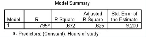
Let us look at a typical SPSS output, as shown in Table 36.31. This table provides the R square. The R square tells us how much variance in the dependent variable is explained by the independent variable in the calculation. First it gives us an R square value of 0.632, which indicates that 63.2% of the variance is accounted for in the model, which is high. The adjusted R square is more accurate, and we advocate its use, as it automatically takes account of the number of independent variables. The adjusted R square is usually smaller than the unadjusted R square, as it also takes account of the fact that one is looking at a sample rather than the whole population. Here the adjusted R square is 0.625, and this, again, shows that, in the regression model that we have constructed, the independent variable accounts for 62.5% of the variance in the dependent variable, which is high, i.e. our regression model is robust. Muijs (2004: 165) suggests that, for a goodness of fit with an adjusted R square:
>0.1 : |
poor fit |
0.11–0.3: |
modest fit |
0.31–0.5: |
moderate fit |
> 0.5: |
strong fit. |
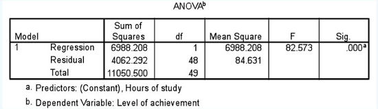
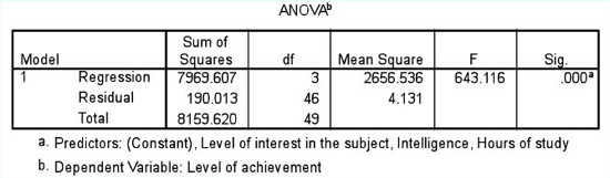
SPSS then calculates the analysis of variance (ANOVA), as shown in Table 36.32. At this stage we will not go into all of the calculations here (typically SPSS prints out far more than researchers may need; for a discussion of df (degrees of freedom) we refer readers to our previous discussion, especially section 36.5). We go to the final column here, marked ‘Sig.’; this is the significance level, and, because the significance is 0.000, we have a very statistically significant relationship (stronger than 0.001) between the independent variable (hours of study) and the dependent variable (level of achievement).
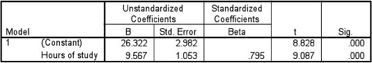
This tells us that it is useful to proceed with the analysis, as it contains important results. SPSS then gives us a table of coefficients, both unstandardized and standardized. We advise to opt for the standardized coefficients, the Beta weightings. The Beta weight (ß) is the amount of standard deviation unit of change in the dependent variable for each standard deviation unit of change in the independent variable. In the example in Table 36.33, the Beta weighting is 0.795; this tell us that, for every standard deviation unit change in the independent variable (hours of study), the dependent variable (level of achievement) will rise by 0.795 (79.5%) of one standard deviation unit, i.e. in lay person’s terms, for every one unit rise in the independent variable there is just over three-quarters of a unit rise in the dependent variable. This also explains why the slope of the line of best fit is steep but not quite 45 degrees – each unit of one is worth only 79.5% of a unit of the other.
TABLE 36.33 THE BETA COEFFICIENT IN A REGRESSION ANALYSIS (SPSS OUTPUT)
Coefficientsa
a. Dependent Variable: Level of achievement
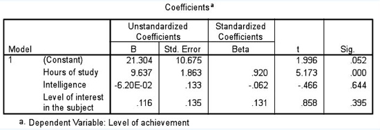
Table 36.33 also indicates that the results are highly statistically significant (the ‘Sig.’ column (0.000) reports a significance level stronger than 0.001). Note also that Table 36.33 indicates a ‘constant’; this is an indication of where the line of best fit strikes the vertical axis, the intercept; the constant is sometimes taken out of any subsequent analyses.
In reporting the example of regression one could use a form of words thus:
a scattergraph of the regression of hours of study on levels of achievement indicates a linear positive relationship between the two variables, with an adjusted R square of 0.625. A standardized Beta coefficient of 0.795 is found for the variable ‘hours of study’, which is statistically significant (ρ<0.001).
In linear regression we were able to calculate the effect of one independent variable on one dependent variable. However, it is often useful to be able to calculate the effects of two or more independent variables on a dependent variable. Multiple regression enables us to predict and weight the relationship between two or more explanatory – independent –variables and an explained dependent –variable. We know from the previous example that the Beta weighting (ß) gives us an indication of how many standard deviation units will be changed in the dependent variable for each standard deviation unit of change in each of the independent variables.
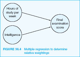
Let us take a worked example. An examination mark may be the outcome of study time and intelligence (Figure 36.4), i.e. the formula is:
Examination mark=ß study time + ß intelligence
Let us say that the ß for study time is calculated by SPSS to be 0.65, and the ß for intelligence is calculated to be 0.30. These are the relative weightings of the two independent variables. We wish to see how many marks in the examination a student will obtain who has an intelligence score of 110 and who studies for 30 hours per week. The formula becomes:
Examination mark

If the same student studies for 40 hours then the examination mark could be predicted to be:
Examination mark

This enables the researcher to see exactly the predicted effects of a particular independent variable on a dependent variable, when other independent variables are also present. In SPSS the constant is also calculated and this can be included in the analysis, to give the following, for example:
Examination mark
=constant+ß study time+ß intelligence
Let us give an example with SPSS of more than two independent variables. Let us imagine that we wish to see how much improvement will be made to an examination mark by a given number of hours of study together with measured intelligence (for example, IQ) and level of interest in the subject studied. We know from the previous example that the Beta weighting (ß) gives us an indication of how many standard deviation units will be changed in the dependent variable for each standard deviation unit of change in each of the independent variables. The equation is:
Level of achievement in the examination
=constant+ß Hours of study+ ß IQ+ß Level of interest in the subject
The constant is calculated automatically by SPSS. Each of the three independent variables – hours of study, IQ and level of interest in the subject – has its own Beta (ß) weighting in relation to the dependent variable: level of achievement.
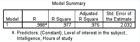
If we calculate the multiple regression using SPSS we obtain the results (using fictitious data on 50 students) shown in Table 36.34. The adjusted R square is very high indeed (0.975), indicating that 97.5% of the variance in the dependent variable is explained by the independent variables, which is extremely high. Similarly the analysis of variance shown in Table 36.35 is highly statistically significant (0.000), indicating that the relationship between the independent and dependent variables is very strong.
The Beta (ß) weighting of the three independent variables is given in Table 36.36 in the ‘Standardized coefficients’ column. The constant is given as 21.304.
It is important to note here that the Beta weightings for the three independent variables are calculated relative to each other rather than independent of each other. Hence we can say that, relative to each other:
the independent variable ‘hours of study’ has the strongest positive effect on (ß=0.920) on the level of achievement, and that this is statistically significant (the column ‘Sig.’ indicates that the level of significance, at 0.000, is stronger than 0.001);
the independent variable ‘intelligence’ has a negative effect on the level of achievement (ß=–0.062) but that this is not statistically significant (at 0.644, ρ>0.05);
the independent variable ‘level of interest in the subject’ has a positive effect on the level of achievement (ß=0.131), but this is not statistically significant (at 0.395, ρ>0.05);
the only independent variable that has a statistically significant effect on the level of achievement is ‘hours of study’.
So, for example, with this knowledge, if we knew the hours of study, the IQ and the level of measured interest of a student, we could predict his or her expected level of achievement in the examination.
To run multiple regression in SPSS, the command sequence is thus: Analyze → Regression → Linear. Send over dependent variable to Dependent box. Send over independent variables to Independent box → Click on Statistics. Tick the boxes Estimates, Confidence Intervals, Model fit, Descriptives, Part and partial correlations, Collinearity diagnostics, Casewise diagnostics and Outliers outside 3 standard deviations → Click Continue → Click on Options → Click on Exclude cases pairwise → Click Continue → Click on Plots. Send over *ZRESID to the Y box. Send over *ZPRED to the X box → Click on Normal probability plots → Click Continue → Click on Save → Click the Mahalanobis box and the Cook’s box → Click Continue → Click OK. For further discussion of the SPSS commands and analysis of output we refer the reader to Pallant (2007: chapter 13) and Tabachnick and Fidell (2007: chapter 5).
TABLE 36.34 A SUMMARY OF THE R, R SQUARE AND ADJUSTED R SQUARE IN MULTIPLE REGRESSION ANALYSIS (SPSS OUTPUT)
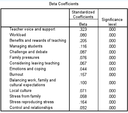
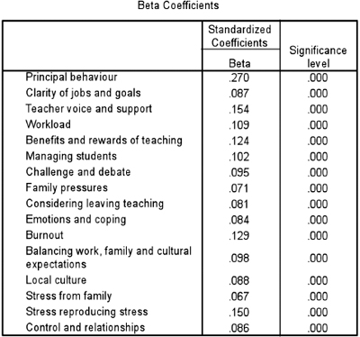
Multiple regression is useful in that it can take in a range of variables and enable us to calculate their relative weightings on a dependent variable. However, one has to be cautious: adding or removing variables affects their relative Beta weightings. Morrison (2009: 40ρ1) gives the example of Beta coefficients concerning the relative effects of independent variables on teacher stress, as shown in Table 36.37.
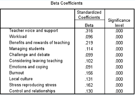
Here one can see the relative strengths (i.e. when one factor is considered in relation to the others included) of the possible causes of stress. In the example, it appears that ‘teacher voice and support’ exert the strongest influence on the outcome (levels of stress) (Beta of 0.323), followed by ‘benefits and rewards’ of teaching (Beta of 0.205), then ‘stress reproducing stress’ (Beta of 0.164) (i.e. the feeling of stress causes yet more stress), followed by ‘burnout’ (Beta of 0.157), ‘managing students’ (Beta of 0.116) and so on down the list. However, if we remove those variables connected with family (‘family pressures’, ‘balancing work, family and cultural expectations’ and ‘stress from family’) then the relative strengths of the remaining factors alters, as shown in Table 36.38.
In this revised situation, the factor ‘teacher voice and support’ has slightly less weight, ‘benefits and rewards of teaching’ have added strength, and ‘control and relationships’ take on much greater strength.
On the other hand, if one adds in new independent variables (‘principal behaviour’ and ‘clarity of jobs and goals’) then the relative strengths of the variables alter again, as shown in Table 36.39. Here ‘principal behaviour’ greatly overrides the other factors, and the order of the relative strengths of the other factors alters.
The point to emphasize is that the Beta weightings vary according to the independent variables included.
Further, variables may interact with each other and may be intercorrelated (the issue of multicollinearity), for example Gorard (2001b: 172) suggests that ‘poverty and ethnicity are likely to have some correlation between themselves, so using both together means that we end up using their common variance twice. If collinearity is discovered (e.g. if correlation coefficients between variables are higher than .80) then one can either remove one of the variables or create a new variable that combines the previous two that were highly intercorrelated’. Indeed SPSS will automatically remove variables where there is strong covariance (collinearity).1 For further discussion of collinearity, collinearity diagnostics and tolerance of collinearity, we refer the reader to Pallant (2007: 156).
The SPSS command sequence for running multiple regression with collinearity diagnostics is: Analyze → Regression → Linear → Statistics → Click ‘Collinearity diagnostics’ → Click ‘Continue’ → Enter dependent and independent variables → In the box marked ‘Method’ click ‘Enter’-> Click OK.
Stepwise multiple regression enters variables one at a time, in a sequence, to see which adds to the explanatory power of a model, by looking at its impact on the R-squared ρ whether it increases the R-square value. This alternative way of entering variables and running the SPSS analysis in a ‘stepwise’ sequence is the same as above, except that in the ‘Method’ box the word ‘Enter’ should be replaced, in the dropdown box, with ‘Stepwise’.
Logistic regression enables the researcher to work with categorical variables in a multiple regression where the dependent variable is a categorical variable. Here the independent variables may be categorical, discrete or continuous. To run logistic regression in SPSS, the command sequence is: Analyze → Regression → Binary Logistic → Insert dependent variable in the ‘Dependent’ box → Insert independent variables into the ‘Covariates’ box → Click on ‘Categorical’ → Move your first categorical variable into the ‘Categorical Covariates’ box → Click the radio button ‘First’ → Click the ‘Change’ button → Repeat this for every categorical variable → Click ‘Continue’ to return to the first screen → Click ‘Options’ → Click the boxes ‘Classification plots’, ‘Hosmer-Lemeshow goodness of fit’, ‘Casewise listing of residuals’ and ‘CI for Exp(B)’ → Click ‘Continue’ to return to first screen → Click ‘OK’. For more on logistic regression we refer the reader to Pallant (2007: chapter 14) and Tabachnick and Fidell (2007: chapter 10).
In reporting multiple regression, in addition to presenting tables (often of SPSS output), one can use a form of words thus, for example (using Table 36.36):
Multiple regression was used, and the results include the adjusted R square (0.975), ANOVA (p<0.001) and the standardized ß coefficient of each component variable (ß = 0.920, ρ<0.001; ß=-0.062, ρ=0.644; ß = 0.131, ρ=0.395). One can observe that, relative to each other, ‘hours of study’ exerted the greatest influence on level of achievement, that ‘level of interest’ exerted a small and statistically insignificant influence on level of achievement, and that; ‘intelligence’ exerted a negative but statistically insignificant influence on level of achievement.
In using regression techniques, one has to be faithful to the assumptions underpinning them. Gorard (2001b: 213), Pallant (2007: 148–9) and Tabachnick and Fidell (2007: 121–8, 161–7) set these out as follows:
The measurements are from a random sample (or at least a probability-based one).
All variables used should be real numbers (ratio data) (or at least the dependent variable must be).
There are no extreme outliers (i.e. outliers are removed).
All variables are measured without error.
There is an approximate linear relationship between the dependent variable and the independent variables (both individually and grouped).
The dependent variable is approximately normally distributed (or at least the next assumption is true).
The residuals for the dependent variable (the differences between calculated and observed scores) are approximately normally distributed.
The variance of each variable is consistent across the range of values for all other variables (or at least the next assumption is true).
The residuals for the dependent variable at each value of the independent variables have equal and constant variance.
The residuals are not correlated with the independent variables.
The residuals for the dependent variable at each value of the independent variables have a mean of zero (or they are approximately linearly related to the dependent variable).
No independent variable is a perfect linear combination of another (not perfect ‘multicollinearity’).
Interaction effects of independent variables are measured.
Collinearity is avoided.
For any two cases the correlation between the residuals should be zero (each case is independent of the others).
Though regression and multiple regression are most commonly used with interval and ratio data, more recently some procedures have been devised for undertaking regression analysis for ordinal data (e.g. in SPSS). This is of immense value for calculating regression from rating scale data.
Pallant (2001: 136) suggests that attention has to be given to the sample size in using multiple regression. She suggests that 15 cases for each independent variable are required, and that a formula can be applied to determine the minimum sample size required thus: sample size ≥ 50+(8 X number of independent variables), i.e. for ten independent variables one would require a minimum sample size of 130 (i.e. 50+80).
Many forms of difference tests and regression analysis with parametric data prefer to work with standardized scores, and we introduce these here. Imagine the following scenes:
A child comes home from school and tells his parents that he scored a mark of 75 for a mathematics test; his parents scold him.
A child comes home from school and tells his parents that he scored a mark of eight for a history test; his parents praise him.
A child comes home from school and tells his parents that he scored a mark of 25 for an English test and a mark of 60 for a physics test; his parents praise him for both.
A child comes home from school and tells his parents that he scored a mark of 80 for a geography test and a mark of 120 for a chemistry test; his parents scold him for both.
How can we explain these apparent discrepant behaviours? In the examples here we do not know the scales used, the range of scores, the means and the distributions around the means. For example the first child who scored 75 for his maths test was scolded because the mean score was 144 and the range was from 75–200, i.e. he scored very low on the test. On the other hand, the child who scored eight for his history test was praised because that was the highest mark in the test, with an average mark of four out of a possible ten, and a range of one to eight. In the case of the child who was praised for scoring two very different marks (25 for English and 60 for physics), this was because the scales and range for the two tests varied, whereas the child who scored 80 for geography and 120 for chemistry was scolded because both tests were marked out of 300 and the average marks for both were 220.
These examples show the need for researchers to compare like with like in using numerical data and scores. We need to know how to judge whether a mark is high or low and how to compare marks between one test and another. Therefore we need to know the scale of the marks, the range of the marks, the mean of the marks, and the distribution of the marks either side of the mean. We need to know how to compare marks from a test which:
uses one scale with marks from a test which uses another scale;
has one range of marks with marks from a test that has another range of marks;
has a mean which is different from the mean of another test;
has a distribution around the mean which is different from the distribution of another test.
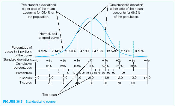
This is addressed by converting scores into standardized scores. Standardizing scores enables the researcher to judge whether a mark is high or low; it enables the researcher to compare marks between one test and another when two different tests have different scales, range, means and distributions around the mean. To standardize scores means to convert them into z-scores. Z-scores have the same mean and standard deviation, even though the original sets of scores had different means and standard deviations, i.e. z-scores let researchers compare scores fairly. A z-score tells us how many standard deviations some-one’s scores lies above or below the mean. By standardizing different sets of scores (usually either a mean of zero and a standard deviation of one), this enables the researcher to compare like with like, to compare scores fairly.
To calculate the z-score we subtract the mean from the raw score and divide that answer by the standard deviation. The formula is thus:
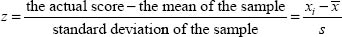
For example if the raw (unadjusted) score is 15, the mean is 10, and the standard deviation is 4, then 15–10 = 5 and 5 ÷ 4 = 1.25. Here the z-score tells us that the person’s score is 1.25 standard deviations above the mean. However, we do not know whether this is a good score, a bad score, or, indeed, what it means. We need to see how this compares with other scores on the same distribution. Figure 36.5 plots the standardized scores on the normal curve of distribution, with the mean score of 0 (zero) and the standard deviation of 1.
Looking at Figure 36.5, in our example, the person who scores 1.25 has scored very well indeed. Had she scored 1 then she would have been better than 84.12 per cent of the population (34.13+34.13 +13.59+2.14 +0.13=84.12): the percentage of people below her (see the lines marked ‘Percentage of cases in 8 portions of the curve’, ‘Cumulative percentages’ and ‘Percentiles’ in Figure 36.5). We know that she is higher than 1 standard deviation above the mean (she has scored 1.25, not 1), so we need to find where her score places her in terms of the rest of the population. For an exact indication of where she stands in relation to the rest of the population we can turn to statistics tables concerning ‘areas under the normal curve’ (on the internet and in the appendices of most statistics books). Then we can simply read off the results (see Table 36.40 for an extract from such a table).
She has a z-score of 1.25, so in Table 36.40 we go to the left-hand column, to the row marked ‘1.2’. Then we go to the column marked ‘0.05’, as this gives us the second decimal place of the ‘1.25’. Then we see the value 0.3944 (emboldened and shaded), i.e. the person is 39.44 per cent above the mean of zero. We know from Figure 36.5 that 49.99 per cent of people are below zero (34.13 + 13.59+2.14+0.13 = 49.99); now we add to that the 39.44 per cent above zero, giving a total of 89.43 per cent. This tells us that, for the person with the z-score of 1.25, only 10.56 per cent (100 per cent minus 89.43 per cent) of the population is above her, so her score is very high.
Using Table 36.40 for another example, if a person receives a z-score of 1.56 then the table gives us a reading of 0.4406, i.e. 44.06 per cent. We know from Figure 36.5 that 49.99 per cent of people are below zero (34.13 + 13.59+2.14+0.13=49.99); now we add to that the 44.06 per cent above zero, giving a total of 94.05 per cent. This tells us that, for the person with the z-score of 1.56 only 4.85 per cent (100 per cent minus 94.05 per cent) of the population is above that score, so the score is extremely high.
An online calculator of this is at: www.danielsoper.com/statcalc/calc02.aspx. This calculator gives the cumulative area under the curve (a figure as a decimal fraction that is less than 1 (let us call it X)). To find the area under the curve beyond that one point simply sub-tract this figure from 1 (the formula, then, is 1 –X) and, for a percentage, multiply it by 100. Another equally straightforward free online calculator of the area under the curve, and the position of a given z-score in that curve is given at stattrek.com/Tables/Normal.aspx.
To calculate z-scores with SPSS, the command sequence is: Analyze → Descriptive Statistics → Descriptives → Variables → Click the box ‘Save standardized values as variables’ → Click OK→ Two new variables will be created of the standardized scores.
Some people are uncomfortable with z-scores, as they do not like negative scores nor do they like an average being 0 (zero). To overcome this, z-scores can be converted to T-scores. To convert a z-score to a T-score, multiply the z-score by 10 and add 50 to the result. For example a z-score of 0.5, multiplied by 10 gives 5, and then, with 50 added, gives 55. The T-score is 55. Many IQ tests and standardized tests convert z-scores. For example a common conversion in IQ tests is to multiply the z-score by 15 and add 100. So a z-score on an IQ test might be 0.5, multiplied by 15 gives 7.5, with 100 added gives 107.5, i.e. the IQ z-score converts to a T-score of 107.5.
Standardized scores are widely used in simple regression, as they enable researchers to compare different sets of scores on a fair basis.
This chapter has introduced several inferential statistics and their related concepts:
measures of difference for parametric data (t-test and ANOVA (one-way, two-way, multiple analysis of variance and post hoc tests of difference);
measures of difference for non-parametric data (Mann-Whitney, Wilcoxon tests, Kruskal-Wallis, Friedman);
the chi-square test of independence and goodness of fit for univariate and bivariate categorical and ordinal variables, as a measure of difference between observed and expected values;
degrees of freedom;
simple regression and multiple regression (typical usage, stepwise regression and logistic regression);
standardized scores and T-scores.
Where relevant, it has also included SPSS command sequences to run these statistics. The statistics covered here are not exhaustive, and, indeed, we introduce several more in the following chapter. However, they do represent the key starting statistics that researchers use.
 Companion Website
The companion website to the book includes PowerPoint slides for this chapter, which list the structure of the chapter and then provide a summary of the key points in each of its sections. In addition there is further information in the form of how to report statistics, a selection of statistical tables, data files and a sample questionnaire for use with a range of statistics in SPSS, plus a full manual on using SPSS, with screen-prints. These resources can be found online at www.routledge.com/textbooks/cohen7e.