Chapter 15
Sequentially Structured REMIC
Sequentially structured REMICs are based on the division of principal and seek to exploit both the market segmentation and liquidity preference theories of the term structure of interest rates.
- Recall, the market segmentation theory asserts that the markets of different maturity bonds are segmented. As a result, the interest rate for each bond is determined by the supply and demand for bonds without consideration given to the expected returns on bonds with different maturities. Under this theory, investors are thought to prefer short-term over long-term bonds. Thus, there is greater demand for short-term bonds and as a result, the price of short-term bonds is higher, resulting in lower yields than those offered by long-term bonds.
- The liquidity preference theory asserts that bonds are perfect substitutes for one another. However, because the investor may be required to sell her bond prior to maturity, thereby assuming interest rate risk, a greater premium is offered to the investor to hold longer-term bonds via higher implied forward rates.
The sequential REMIC waterfall bondlabSEQ cash allocation rules may be expressed as follows:
- { Pay 100% of available interest to each class on a pro-rata basis, based on each class's respective accrued interest }
- { Pay 100% of available principal in the following order: }
- { Tranche 1 until the outstanding balance is reduced to zero, }
- { Tranche 2 until the outstanding balance is reduced to zero, }
- { Tranche 3 until the outstanding balance reduced to zero, }
The deal pricing speed is 125 PSA. Table 15.1 provides a comparative analysis between the collateral, Tranche A, Tranche B, and Tranche C. The astute reader will notice the following:
- The sum of the coupon interest paid to the bond holders is less than that derived from the underlying collateral.
- The proceeds, as shown in Table 15.1, are less than the cost required to accumulate the collateral.
Table 15.1 REMIC Sequential Analysis
| MBS 4.00% | Tranche A | Tranche B | Tranche C | |
| Net Coupon | 4.00% | 0.63% | 1.41% | 2.72% |
| Note Rate | 4.75% | 4.75% | 4.75% | 4.74% |
| Term | 360 mos. | 360 mos. | 360 mos. | 360 mos. |
| Loan Age | 0 mos. | 0 mos. | 0 mos. | 0 mos. |
| Orig. Bal. | $50mm | $75mm | $75mm | |
| Price | $105.75 | $100.00 | $100.00 | $100.00 |
| Yield to Maturity | 3.26% | 0.63% | 1.41% | 2.71% |
| Spot Spread | 1.33% | 0.18% | 0.07% | 0.24% |
| Pricing WAL | 9.81 | 2.19 | 6.91 | 17.40 |
| First Principal Pmt | 1-2013 | 01-2013 | 11-2016 | 08-2023 |
| Last Principal Pmt | 1-2043 | 11-2016 | 08-2023 | 11-2042 |
| Modified Duration | 7.72 | 2.17 | 6.56 | 13.7 |
| Convexity | 49.9 | 3.91 | 26.50 | 110.00 |
| Effective Duration | 7.13 | 1.78 | 8.97 | 13.7 |
| Effective Convexity | −15065 | 1377 | −18941 | −49830 |
In order to improve deal execution, the dealer may create an additional “IOette” class that represents the excess of the underlying collateral's interest payments over those paid to that of tranches A, B, and C. For purposes of this discussion, assume the existence of an additional IOette class whose valuation is sufficient to create a profitable arbitrage. Later, in Chapter 17, we will review the structuring and valuation of the IOette class.
The sequential structure alters the timing of the principal cash flow to the investor. Namely, Figure 15.1 and Table 15.1 show that Tranche A receives cash flows from Jan 2013 to Nov 2016, while Tranches B and C are said to be locked out. That is, principal is paid to these tranches only after the preceding tranche's principal balance is reduced to zero. For example, Tranche B's payment window, given a 125 PSA pricing speed, begins in Nov 2016 and ends Aug 2023. Tranche C's payment window begins in Aug 2023 and ends in Dec 2042 (recall section 7.2.2).
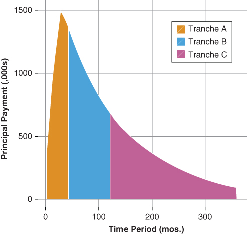
Figure 15.1 Sequential Principal Cash Flow Diagram
Time tranching is parsing the timing of the return of principal to the tranches. It changes the average life profile of each tranche relative to the underlying collateral. As shown in Table 15.1, both Tranche A and Tranche B report a shorter average life than the underlying collateral, which is 9.81 years. Tranche C reports a longer average life than the underlying collateral at 17.4 years. The dealer, by structuring tranches with a shorter average life than the collateral, is exploiting both the market segmentation and liquidity preference theories of the term structure of interest rates, discussed earlier in sections 2.2 and 2.3, thereby creating a positive arbitrage.
A sequential transaction relies on the division of principal to create each tranche. As a result, both call risk and extension risk are asymmetrically distributed across the transaction's capital structure. The fast-pay tranches bear greater call risk relative to either the underlying collateral or the last cash flow tranche. Conversely, the penultimate and last cash flow tranches bear greater extension risk relative to either the underlying collateral or the fast-pay tranche.
At first blush, one may view the fast-pay tranche (Tranche A) as the tranche bearing the brunt of prepayment risk. However, it is not the case that the fast-pay tranche is subject to greater call risk. Rather, it is the last cash flow tranche that bears the greater prepayment risk relative to either the underlying collateral or the fast-pay tranche. Stated differently, the risk that the realized prepayment rate will deviate over time from the assumed pricing speed has a higher probability of occurring in the tranches that have a longer average life compared to those with shorter average life. As a result, the last cash flow tranche exhibits greater average life variability than the first or fast-pay tranche.
15.1 Key Rate Duration Analysis
Key rate duration analysis illustrates how the allocation of principal across time (time tranching) impacts each security, further reinforcing the points above. Figures 15.2 and 15.3 provide a side-by-side comparison of both the collateral and Tranche A's key rate duration. Notice the following:
- The collateral's key rate durations are heavily concentrated along the longer key rate tenors, whereas Tranche A's key rate durations are heavily concentrated along the shorter key rate duration tenors. Thus, Tranche A has greater price risk relative to the shorter tenors of the curve than that of the underlying collateral.
- Tranche A's 10-year key rate duration is less than half that of the collateral's 10-year key rate duration. Recall the forward mortgage rate, which determines borrower prepayment rates, is a function of the forward 2- and 10-year swaprates. Thus, Tranche A's lower 10-year key rate duration reflects not only its shorter average life but also its lower sensitivity to mortgage prepayment rates. Furthermore, the key rate duration analysis clearly shows Tranche A's price sensitivity to shorter key rate durations is greater than that of the underlying collateral, suggesting a greater overall price sensitivity to the shorter end of the term structure.
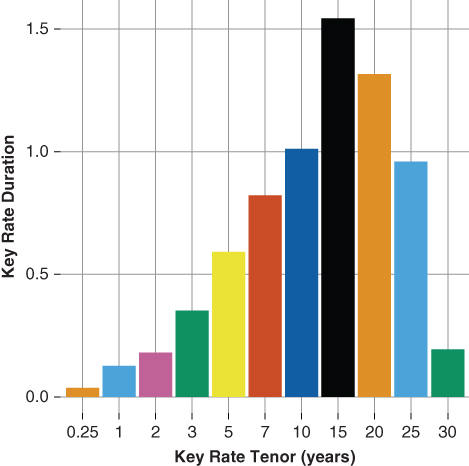
Figure 15.2 Key Rate Duration MBS 4.00%
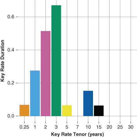
Figure 15.3 Key Rate Duration Tranche A
Figures 15.4 and 15.5 provide key rate duration analysis for both Tranche B and Tranche C. Figure 15.4 shows Tranche B's 10-year key rate duration is four times that of the underlying collateral, whereas tranche C's 10-year key rate duration is less than one-quarter that of the underlying collateral. The key rate duration analysis highlights the following:
- Tranche B is highly leveraged against the 10-year swap rate relative to either the underlying collateral or Tranches A or C. As such, Tranche B represents the fulcrum of the transaction.
- Tranche C's 10-year key rate duration is less than that of the underlying collateral or Tranche B. However, the longer key rate durations are significantly higher, suggesting Tranche C is most sensitive to the longer tenors of the term structure and prepayment expectations. Consider the following, the term structure flattens between the 10- and 30-year maturities (a bull flattening of the yield curve), which, in turn, leads to a lower forward mortgage rate and higher forward prepayment expectations. Conversely, a steepening between the 10- and 30-year maturities (a bear steepening of the yield curve) leads to a higher forward mortgage rate and lower forward prepayment expectations.
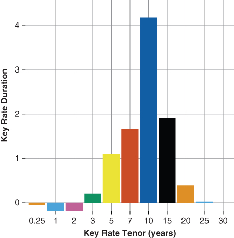
Figure 15.4 Key Rate Duration Tranche B

Figure 15.5 Key Rate Duration Tranche C
Taken together, Table 15.1 and Figures 15.2 though 15.4 indicate, all else equal, Tranche C, after giving consideration to effective duration, is more negatively convex than both the underlying collateral and Tranches A or B.
15.2 Option-Adjusted Spread Analysis
The OAS analysis presented in Table 15.2 further illustrates the impact of time tranching on the valuation of MBS cash flows. Notice, Tranche C, the last cash flow tranche, OAS is higher than that of either Tranche A or B, indicating the investor receives addition compensation, in the form of a higher OAS, for accepting the greater negative convexity of Tranche C—further reinforcing the notion that the last cash flow tranche bears greater relative prepayment risk.
Table 15.2 REMIC Sequential OAS Analysis
| MBS 4.00% | Tranche A | Tranche B | Tranche C | |
| Net Coupon | 4.00% | 0.63% | 1.41% | 2.72% |
| Note Rate | 4.75% | 4.75% | 4.75% | 4.75% |
| Term | 360 mos. | 360 mos. | 360 mos. | 360 mos. |
| Loan Age | 0 mos. | 0 mos. | 0 mos. | 0 mos. |
| Price: | $105.75 | $100.00 | $100.00 | $100.00 |
| Yield to Maturity | 3.26% | 0.63% | 1.41% | 2.70 |
| OAS | 0.52% | 0.00% | 0.05% | 0.31% |
| ZV-Spread | 1.28% | 0.00% | 0.00% | 0.27% |
| Spread to the Curve | 1.52% | 0.26% | 0.11% | 0.35% |
| Effective Duration | 7.13 | 1.78 | 8.97 | 13.7 |
| Effective Convexity | −15065 | 1377 | −18941 | −41132 |
The degree to which each tranche is leveraged against the underlying collateral prepayment rate will determine its convexity and valuation. Those tranches most leveraged against the underlying collateral's prepayment rate will typically exhibit greater relative negative convexity, and naturally trade to a higher yield and OAS than those with less relative leverage and more positive convexity. Option-adjusted spread analysis aids the investor in estimating the value of the embedded prepayment option across structures.
15.3 Weighted Average Life and Spot Spread Analysis
The investor may gain additional insight by examining the results of the short-rate simulation. In particular, the weighted average life distribution allows the investor to visually examine how the allocation of principal influences each tranche's average life profile. Further, examining the spot spread distribution yields additional insights relating to the allocation of principal and its impact on cash flow valuation.
15.3.1 Tranche A—WAL and Spot Spread Distribution Analysis
Figures 15.6 and 15.7 compare the weighted average life distribution of the underlying collateral to that of Tranche A. Notice, across all short-rate trajectories the WAL of Tranche A is shorter than that of the underlying collateral. Furthermore, the WAL is also less than that reported using the transaction pricing speed of 125 PSA, indicating the prepayment model is forecasting a faster near-term prepayment rate than the prepayment assumption used to price the transaction.
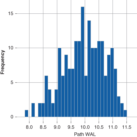
Figure 15.6 WAL Dist. MBS 4.00%
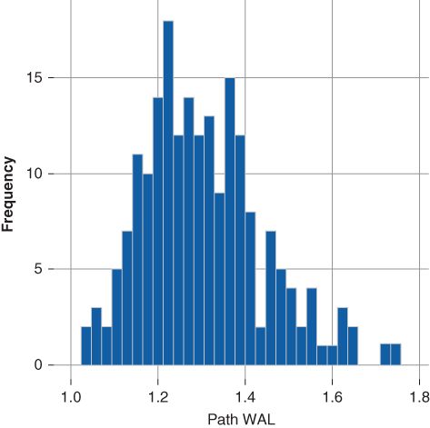
Figure 15.7 WAL Dist. Tranche A
As a result of the model's faster prepayment forecast and consequently shorter WAL the spread to the curve declines. Additionally, the ZV-spread is less than both the spread-to-the curve using the prepayment model (0.26%) and the nominal pricing spread (0.25% over the 2-year swap rate). Thus, by the valuation framework outlined in Chapter 4, Tranche A's rich-priced cash flows outweigh the cheap-priced cash flows. The low ZV- and OA- spreads in Table 15.2 result from a loss of coupon income due to faster prepayment expectations relative to the transaction's pricing speed.
Figure 15.8 provides additional insight. Recall, the ZV-spread is calculated as the average of the spot spread realized along each short-rate trajectory. The distribution of the spot spread along each path illustrates how the cash flow valuation changes given the short-rate trajectory and its impact on the estimated borrower prepayment vector given by the prepayment model.
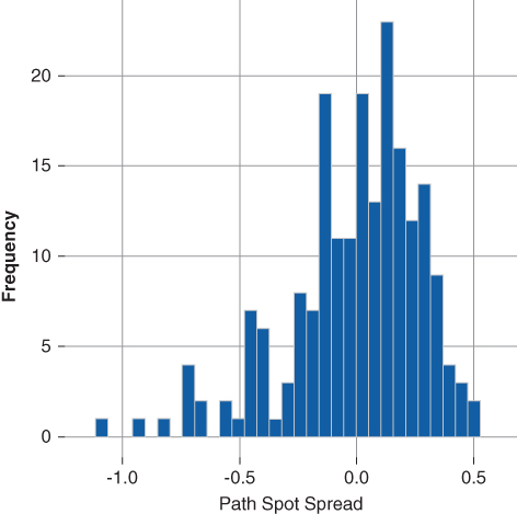
Figure 15.8 Tranche A—Spot Spread Distribution
The spot spread distribution ranges from a low of −1.09% to a high of 0.49% while the average, ZV-spread, is 0.00%. Short-rate trajectories resulting in faster prepayment vectors will act to shorten Tranche A's average life and reduce the coupon income received by the investor. In turn, a lower path spot spread results. Conversely, those trajectories resulting in slower prepayment vectors extend Tranche A's average life and increase the coupon income received by the investor. These paths result in a higher path spot spread. The left skew of Tranche A's spot spread distribution illustrates the extent to which the tranche is callable (negative spot spreads). Analysis of the spot spread distribution aids the investor in quantifying the extent to which Tranche A's call risk influences the overall valuation of its cash flows.
15.3.2 Tranche B—WAL and Spot Spread Distribution Analysis
Given a 125 PSA pricing speed the average life of the underlying collateral is 9.81 years and the average life of Tranche B is 6.91 years (Table 15.1). Tranche B's weighted average life distribution, as shown in Figure 15.9, reports less relative extension risk than the underlying collateral (Figure 15.6). Specifically, the maximum weighted average life of Tranche B is 7.95 years while that of the collateral is 11.49 years. Similarly, Tranche B exhibits greater relative call risk than the underlying collateral. Its minimum average life is 4.70 years versus the underling collateral minimum average life of 7.93 years. The average life distribution analysis confirms the finding in Table 15.2, which indicates Tranche B is more negatively convex than the underlying collateral.
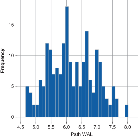
Figure 15.9 WAL Dist. Tranche B
Figure 15.10 presents Tranche B's spot spread distribution. Again, the distribution is negatively skewed and reports an average of 0.00%. Notice, the extreme value in the left tail of the distribution. The minimum spot spread is −2.21%, which accounts for the zero average ZV-spread and indicates that Tranche B also has embedded call risk. The maximum spot spread is 1.01%.
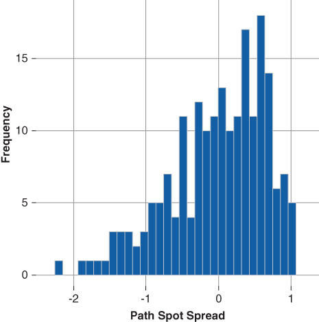
Figure 15.10 Spot Spd. Dist. Tranche B
Tranche B reports a greater relative negative convexity than that of the underlying collateral and that of Tranche A. However, Tranche B's extension risk is minimized by the presence of Tranche C; the last cash flow Tranche. The allocation of principal to the last cash flow tranche minimizes, in absolute terms, the extension risk of Tranche B.
15.3.3 Tranche C—WAL and Spot Spread Distribution Analysis
Figures 15.11 and 15.12 illustrate the weighted average life and spot spread distributions for Tranche C. Notice, the WAL and spot spread distributions exhibit less skewness than those of either Tranche A or B. Overall, Tranche C's weighted average life profile exhibits greater relative stability as does its spot spread distribution. Recall Figure 15.5, key rate duration analysis, C exhibited a much lower key rate duration at the 10-year tenor than either A or B. However C exhibits greater key rate duration exposure beyond the 10-year tenor. Hence, one would expect C to exhibit greater sensitivity to both longer tenor interest rates as well as expected borrower prepayment rates.
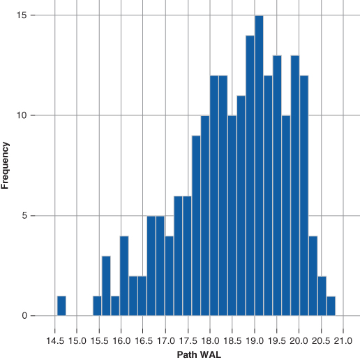
Figure 15.11 WAL Dist. Tranche C
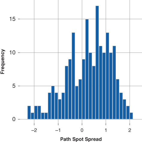
Figure 15.12 Spot Spd. Dist. Tranche C
15.4 Static Cash Flow Analysis
Often the investor employs static cash flow analysis as a simple yet effective filter for eligible securities. Investment guidelines may specify a maximum allowable maturity. For example, a bank's portfolio investment guidelines may state the average life or maturity of any investment cannot exceed seven years. In this case, as part of the screening process the portfolio manager may employ static cash flow analysis such as that shown in Figure 15.13 to test the eligibility of each tranche based on its average life profile. The static cash flow analysis in Figure 15.13 presents the average life of each sequential tranche given PSA assumptions ranging from a low of 50 PSA to a high of 350 PSA. Given the bank's investment guidelines:
- Tranche C is considered an ineligible investment since under all PSA assumptions its average life is beyond the seven-year limit.
- Trance B is also ineligible since is average life extends beyond the seven year limit under both the 50 and 100 PSA scenarios.
- Tranche A is an eligible investment since its average life is under seven years across all PSA scenarios and the portfolio manager may conduct further analysis against competing investment alternatives.
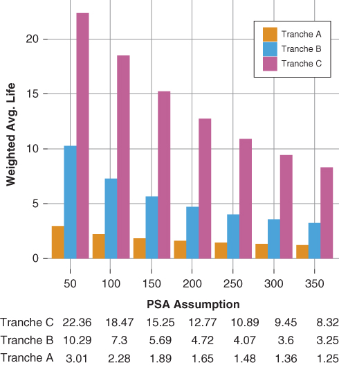
Figure 15.13 Average Life Analysis
Alternatively, a life insurance company's investment guidelines may set a eight-year minimum maturity or average life in order to fund longer dated liabilities—such as a pension buyout. Given the insurance company's guidelines:
- Tranche C is an eligible security and the investor may conduct further analysis on the relative value merits of Tranche C versus competing investment alternatives.
- Both tranches B and C are ineligible securities since their average lives are less than eight years under most PSA scenarios.
Both examples presented above suggest there is a degree of market segmentation (section 2.2) on the part of institutional investors. In each case, market segmentation is primarily motivated by each institution's unique liability stream. Dealers are able to create securities that meet each institution's portfolio guidelines by time tranching cash flows through the allocation of principal.