Chapter 9
Modelling Software Processes
There are many needs that can well be met by applications that are organised as processes. So, having considered how we can describe different properties and attributes of software, both formally and informally, we now bring together ideas about architectural style and modelling to consider how we can model the characteristics of an application that is to be implemented as a process.
This chapter provides a fairly generic summary of how to model the different aspects of this relatively simple form of software element, since processes can be organised and implemented in different ways, and can be realised in a range of architectural styles. Indeed, an important thing to remember is that a distinctive characteristic of software is that a ‘one size fits all’ approach is definitely inappropriate, and that the choice of modelling forms to use needs to be adapted to the particular form of ISP being addressed.
9.1Characteristics of software processes
In order to model software processes, it helps to have a fairly clear idea of just what is meant by a ‘process’. From the perspective of an operating system, a process can be considered as being an executable block of code and associated data, that is created from some user-owned software application and is executed as a single thread of control. This interpretation can be seen as being closely related to the way that the underlying computer operates, and so historically, was a form widely used in early computing applications, and is still widely used today.
At its most simple, and most closely related to the structures of the underlying processor, this can be implemented by using a call-and-return architectural style. This interpretation also fits quite well with such architectural forms as communicating-processes, where an application might be formed by using multiple processes, perhaps operating in a pipe-and-filter manner, with each performing its task and then passing the outcomes on to the next one. However, since the individual processes in a communicating process structure may well be implemented by using call-and-return, we will focus on modelling this type of process in the rest of this chapter.
The key point about a process is that it has a single thread of control. Execution of a process begins with the first instruction, and follows a single sequence or path through the instructions. That sequence may be different each time it executes of course, depending on data and other factors, but for the ‘main’ program element, and for any sub-programs, execution will always begin at the first statement.
Figure 9.1 shows a very simple illustration of this for a program made up from a main body and two sub-programs (A and B). On this occasion, sub-program A is invoked twice, the second time exiting from an intermediate point, with the thread of control, shown as a dashed line, forming a single path.
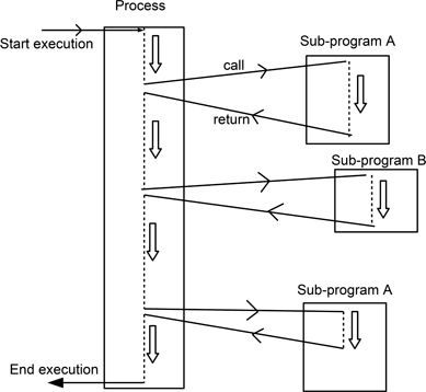
Figure 9.1: Simple illustration of a single thread of control
So, how can we model the way that this is organised in the abstract? The functional viewpoint can be used to describe the task that the process is performing, and the constructional viewpoint can be used to indicate how the tasks and sub-tasks involved are organised, as well as any issues related to data access. Additionally, the behavioural viewpoint may also aid with modelling how the process interacts with the external world, and the data modelling viewpoint can be used where there are important relationships in the data that may have an influence upon the structure of the process.
The issue of data organisation may be rather implementation-specific. For many programming languages permanent data storage can only be provided where variables are declared in the ‘main’ body of the program, with variables declared in the sub-programs only being created when that sub-program is executing. This means that knowledge about the structure, format and values of any data involved will be global in nature and shared among the elements of a process.
A disadvantage of this sharing of knowledge about data is that it forms a technical debt that can impede later evolution of an application. This issue was demonstrated by David Parnas (1972), with his ideas later being extended in (Parnas 1979). His crucial insight that systems constructed around information hiding, whereby the detailed form of data elements was only known to a few key parts of a system, made it easier to change software was a very important one, and one that underpinned the emergence of the object-oriented paradigm. (Of course, there is a trade-off, in that using this approach can be expected to result in a more complex set of structures for the organisation of the process, in order to maintain this concealment of detail.)
While information-hiding is associated with the object-oriented paradigm and the concept of encapsulation, it is worth noting that in (Parnas 1972) the example solution was presented as a top-down design for a process. So constructing single-threaded processes around information hiding is certainly possible, but few procedural programming languages really provide explicit support for its use.
9.2Modelling function: the data-flow diagram (DFD)
The design of processes commonly begins with the functional viewpoint, since this fits well with the idea of a single thread of control that involves specifying what the process is to do. Modelling the functional aspects of a process has a domain-oriented element and hence has clear links to requirements specification activities. One way of describing function is to do so in terms of the way that different actions performed by the process interact with the various forms of information (data) that form a necessary part of the task of an application. Hence, what is usually termed the data-flow perspective, mixing actions and data, is one that has provided a highly effective way to describe the functional viewpoint for many different domains.
The data-flow approach to modelling function probably long pre-dates the use of digital technology, and it is thought such forms may well have been used in the 1920s to model the way that teams of workers in businesses were organised when performing their tasks (Page-Jones 1988). This may or may not have been the case (the evidence seems to be largely folklore), but the point remains that data-flow forms can be used to model many data-driven activities performed by people (such as processing insurance claims, or assembling flat-pack furniture) just as effectively as they can be used for modelling the activities performed by software and their interactions with data.
The name might be thought to imply that a DFD is primarily concerned with the data-modelling viewpoint, but the real issue here is describing the operation of a system from the perspective of the transfer of information, rather than being concerned about its form. DFDs are not really concerned with modelling the form of the data, but the fact that they are concerned about how it is used does suggest that they do incorporate some element of the data-modelling viewpoint.
When we look at plan-driven approaches to creating design models in Chapter 13, we will see that DFDs formed a popular starting point for many early approaches, ultimately mapping on to call-and-return implementations (Wieringa 1998). However, that doesn't mean that they can't be used with other architectural forms or development strategies (for example, they fit quite well with service-oriented architectures). In particular, where an application is strongly data-centric, they have the benefits of being:
easy to sketch and comprehend (so, handy for describing ‘user stories’);
useful for clarifying what an application should do, and identifying any dependencies upon other processes or information that this may involve.
DFDs can also be drawn with a range of degrees of formality. The ‘bubble’ form we use here, as popularised by Tom De Marco (1978) is relatively informal and easy to sketch. This is partly because it also makes good use of different shapes to differentiate between the elements making up a diagram (Moody 2009). In contrast the syntax employed for DFDs in the SSADM (structured systems development and analysis method) (Longworth 1992), is rather more formal and ‘documentation-oriented’ (see Chapter 14).
While DFDs are often thought of as being used to describe complete applications, there is really no reason why they should not be used more selectively to help clarify and understand elements of an application or its requirements. Regardless of the scope of a DFD, the top level of this is normally referred to as the context diagram, consisting of a single ‘bubble’ linked to a set of external sources and sinks of information. This is illustrated in Figure 9.2, which shows a context diagram for the operation of withdrawing cash from a ‘hole-in-the-wall’ dispenser.
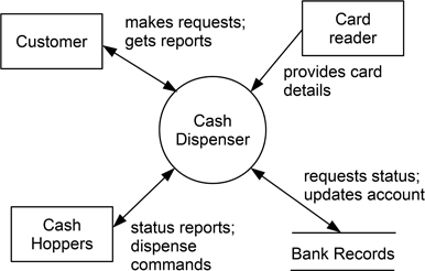
Figure 9.2: The context diagram for a cash withdrawal
This illustrates the four main symbols used in a DFD: the circle or ‘bubble’ denoting an operation; an arc indicating data flow (usually labelled with the form of data involved); parallel bars to show the use of some form of data store; and a box used to indicate the involvement of an external source or sink of information.
Turning now to the CCC, the box below shows the first steps in modelling a client request to book a car.
In expanding the context diagram to produce a more detailed and comprehensive model, we need to ensure that the next level of diagram will use the same inputs and outputs (of course, in the spirit of ISPs, it might be that in thinking about this, the designer realises that the context diagram doesn't cover all issues). Figure 9.3 provides an expanded DFD for the process of booking a car. Note that control issues are not described, so where, as in Bubble 5 reserve car, there might be two possible outcomes, depending on whether or not the chosen car has been booked out to someone else while the user is making their choice, we just draw all possible outcomes and use the text in the bubble to indicate that a choice occurs.
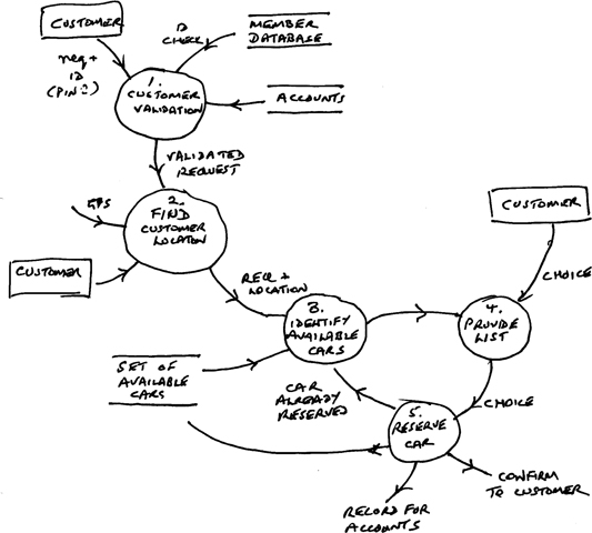
Figure 9.3: An expanded DFD for booking a car
(There is also the possibility that no car is available. This option can be considered as being included under confirm to customer, but it is poor practice to make such actions cover compound issues. So there should probably be another exit bubble to cope explicitly with the possibility that either no cars are available in the vicinity, or that there are no cars available by the time that the customer has made a choice—the reader might like to extend the diagram to handle this.)
A strength of DFDs is that they are intrinsically hierarchical. We can take one bubble (for example, 3. Identify available cars) and expand this as a further, more detailed DFD. The bubbles in this new diagram will be numbered as 3.1, 3.2 etc. Being able to do this helps with managing the cognitive load of thinking about function, since the designer only needs to consider a limited set of actions at any point. At the same time, the resulting ‘tree’ of diagrams aids navigation around the design model at different levels of detail.
When developing a DFD, it is useful to start by modelling the ‘physical’ world (in our case, cars and customers) and then later seek to describe this more abstractly in terms of system functions as we move on to consider mapping the model on to software elements. (The corresponding DFDs are referred to as ‘physical DFDs’ and ‘logical DFDs’ respectively.) And as a final comment upon creating DFDs for the present, it is worth observing that while layout can be a bit of a challenge (as with any such diagram), the same philosophy should apply as when sketching in general. Don't worry if the diagram has things like crossing flow lines—if the diagram does become too messy and this begins to obscure the ideas it incorporates, it may be worth redrawing it, but otherwise, leave this task until later.
Figure 9.3 emphasises the issue of there being a single thread of control. For any booking action there will be a single path through the DFD. The DFD can also be used with scenarios of use (Ratcliffe & Budgen 2001, Ratcliffe & Budgen 2005) that define the conditions for specific execution paths, and which can also be combined with user stories both for developing and validating the DFD.
DFDs are easy to sketch, and as in the examples above, they do not necessarily need to be large and complex. They also provide a tried and tested way of thinking about the functions of a process. However, they implicitly assume the widespread availability of knowledge about the data, and so are less suited to modelling the encapsulation of data needed with object-oriented architectures.
9.3Modelling behaviour: the state transition diagram (STD) and the state transition table (STT)
The idea of state is quite a familiar one. As an everyday example, we think of ourselves as being in a sleeping state when we are asleep, and in an awake state when we are not sleeping. And there are events causing transitions between these that are familiar to us, such as that caused by an alarm clock, or listening to a dull speaker in a warm room! We might also identify some other related states such as day-dreaming or dozing, which can be considered as being sub-states of a major state (in this case awake). This is shown as a simple model in Figure 9.4.
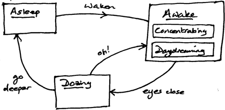
Figure 9.4: An everyday state model
Within computing, some classes of problem (and solution) can usefully be described and modelled by treating them as a ‘finite-state machine’. Such a model can be considered as one that describes a running application as being in one of a finite set of possible states, with external (and internal) events providing the triggers that can lead to transitions occurring between those states.
A process (as well as a data element or object) in a computer fits this quite well. In a formal sense, the ‘state’ of a process at any point can be fully described in terms of the contents of any variables that it uses, and the ‘program counter’ that determines which instruction is to be executed next, although we usually prefer to use rather more abstract descriptions of state. And using a finite-state form of description to think about the properties of a process enables us to model the ‘rules’ which govern its behaviour. Indeed, an important aspect of such models is that they not only describe the transitions that are allowed to occur, but also those that should not be able to happen. And of course, as a general constraint, an entity can only be in one state at any time.
We have already seen an example of state modelling when describing the different states that one of the cars owned by CCC can be in. A car can be available, reserved, or unavailable. This is quite a simple model, and doesn't really allow us to describe some of the situations that might arise, such as when a car is unavailable because it is damaged, or needs servicing. While that can be considered as being unavailable as far as modelling customer activities is concerned, it isn't really sufficient to meet all of the needs of the CCC. (And, as we saw when considering the DFD for booking a car, what should happen when two customers are offered the same car, when it is near to both of them?)
Figure 9.5 shows an example of a state transition diagram that provides a slightly more comprehensive model that describes the different states of a car. It uses the notation developed by Ward & Mellor (1985) in which there are four principal components.
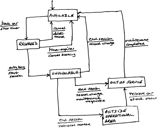
Figure 9.5: An extended state model for a car as an STD
A state represents an externally observable mode of behaviour for some entity, and is represented by a box which is labelled to indicate that behaviour.
A transition is described by an arrow, identifying a ‘legal’ change of state that can occur within the entity.
The transition condition that identifies the condition(s) that can lead to a transition are written next to the arrow, above the line.
The transition action is written by the arrow, but below the line, and describes any actions that may occur as a result of the transition. There may be several of these, and they might occur in a sequence or simultaneously.
This model has two states that are additional to the original set, reflecting the possibilities that at the end of a session a car may require maintenance (perhaps because a routine service is due, or simply because the fuel level is too low); and that it might have been left outside of the area covered by the CCC, and require retrieval. Both of the new states can be considered as being forms of unavailable, a point we will return to later.
We have modelled the car as an STD in this instance, but could equally well model something ‘active’ such as an application or process. The value of using state modelling is that it creates a behavioural model that can be used to complement the functional model provided by using a form such as a DFD. For example, a state model can help with clarifying the ‘rules’ that determine which choices can be made when the process executes. There are no hard and fast rules about how and when to use an STD when modelling processes. It may be useful to begin by creating a very abstract ‘system-wide’ STD to help thinking about the functional tasks that the process needs to perform. Or it may be helpful at a later stage to use an STD to focus ideas about how some aspect of the application needs to behave (such as the example above of modelling the car).
Modelling the behaviour of a process (or more likely, specific elements of it) in this way provides both a means of augmenting the design model as well providing a means of performing consistency checking that all options have been considered. Essentially it is supplementary, since it doesn't usually lend itself to helping with developing the constructional model in the way that occurs with a DFD (we discuss this more fully in Chapter 13). In particular, STDs are not hierarchical in form and so for practical reasons, they are likely to be most effective when used to model elements of an application's task.
Figure 9.6 provides a further example showing a rather more complex (but still incomplete) model, in this case for the behaviour of an aircraft forming part of an air traffic control system. The short arrow at the top indicates the initial state (when the aircraft first enters the airspace and is detected by the primary radar). There are two sources of complexity here: one is the number of actions that an aircraft might take (including flying through the airspace and onwards, being stacked etc.) and the other is the number of operations (actions) performed in each transition (this is simplified here of course).
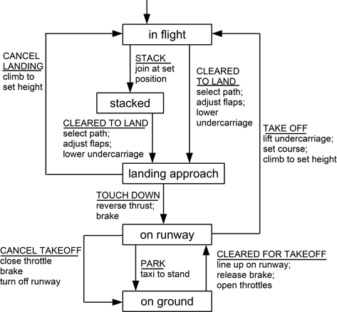
Figure 9.6: An example of an STD modelling aircraft behaviour
While STDs provide a useful visual description of how entities in a model change their state, and the operations that are involved in those changes, as well as being easily sketched, the lack of a hierarchical decomposition means that they can rapidly become inconveniently complex in form. An alternative, but less visual, way of presenting this information is to use a table, known as a state transition table or STT. A common convention for these is to plot the set of states down the left-hand column, and then the set of events as the column headers for the remaining columns. Entries in the table can describe both the actions to be performed and also the final state that results when a particular event occurs for a given initial state.
As an example, the model in Figure 9.5 is shown in tabular form in Table 9.1. While a state transition table provides essentially the same model as an STD (or can be used to do so), it can more easily be used where it is necessary to handle issues of scale, or of many possible transitions between a relatively small number of states.
Make booking |
End of session |
Entry key used |
20 minute time-out |
|
Available |
Record the booking; start 20 min timer; change to reserved status |
|||
Reserved |
Refuse booking |
Cancel booking and return to available status |
Record start time of session and location; change to unavailable status |
Notify user of cancelled booking; change to available |
Unavailable |
Refuse booking |
Record end time and location; change to available mode |
Additionally, the issues of verification and validation can be more systematically addressed through analysis of an STT (‘are we building the system right’ and ‘are we building the right system’) (Boehm 1981). An STT makes explicit those situations where we do not expect there to be a response to a specific event, since these correspond to an empty cell, and even as simple an act as checking and justifying all empty entries can be a useful form of analysis. In particular, when there is a need to discuss these with the ‘customer’, tabulation may be easier to use than diagrams—software engineers draw diagrams all the time, but others might be less comfortable with their use.
9.4Modelling data: the entity-relationship diagram (ERD)
The data-modelling viewpoint also plays a rather subsidiary role when modelling processes, except of course, when a process is an element in an application that has an overall data-centric style. A form that is widely for modelling the relationships that exist between static data elements in a specification model or a design model is the entity-relationship diagram (ERD). While the entity-relationship concept has provided an essential foundation for the development of the models that underpin many database systems, it can help with modelling detailed data models for less data-centric applications too (Page-Jones 1988, Stevens 1991). As we will see in the next chapter, the form of the ERD has also provided useful ideas for modelling object relationships.
As with all of the notations covered in this chapter (and elsewhere) there are various, largely syntactic, variations in the way that ERDs are presented visually. However, many forms seem to have been derived from the pioneering notation devised by Peter Chen (1976). Here we concentrate on the essential elements, avoiding the more detailed nuances of the form.
Figure 9.7 shows the three principal symbols that are used in ERDs, together with their meanings (the symbols for entities and relationships are fairly universal). These entities are defined as follows:
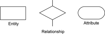
Figure 9.7: The basic entity-relationship notation
entities are real-world ‘objects’ that have common properties;
a relationship is a class of elementary facts that relates two or more entities;
attributes are classes of values that represent atomic properties of either entities or relationships (the attributes of entities are apt to be more readily recognised than those of relationships, as can be seen from the examples).
We might usefully note that the ERD, like the DFD, makes good use of visual differences to clearly distinguish between the symbols.
The nature of an entity will, of course, vary with the level of abstraction involved within a design model. Entities may also be connected by more than one type of relationship. (For example, the entities student and teacher might be connected by both of the relationships attends-class-of and examines.) Also, attributes may be composite, with higher-level attributes being decomposed into lower-level attributes. (As an example of this, the abstract attribute course-module might be decomposed into module-number, module-title and learning-level.)
Relationships are also classified by their ‘n-ary’ properties. Binary relationships link two entities. An example of a binary relation is the relationship ‘reserves’ that will exist between the entities CCC member and car (it isn't physically possible to drive more than one car at any moment!). Figure 9.8 shows some simple relationships that exist in the CCC. Relationships may also be ‘one to many’ (1 to n) and ‘many to many’ (m to n). Examples of these relationships are:
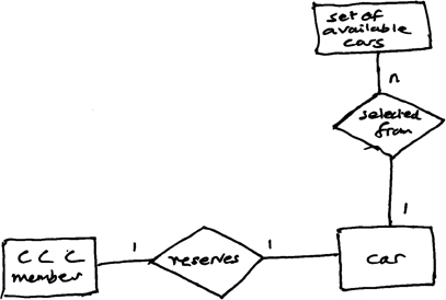
Figure 9.8: Some entity-relationship links in the CCC
car (of order 1) selected from the set of cars (entity of order n) provided in a city
authors (n) having written books (m)
(In the latter case, an author may have written many books, and a book may have multiple authors.) The effect of the n-ary property is to set bounds upon the cardinality of the set of values that are permitted by the relationship.
The development of an ERD typically involves performing an analysis of specification or design documents, and classifying the terms in these as entities, relationships or attributes. The resulting list then provides the basis for developing an ERD.
Figure 9.9 provides an ERD model for the entities that might be involved in an air traffic control system (following on from the example in the previous section). This example can be considered as being quite design-related, and provides supplementary information about the factors that need to be considered in the eventual design model. The relationship between aircraft and runway also provides a simple illustration of a point that was made earlier, concerning the possible existence of multiple relationships between two entities.
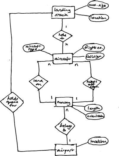
Figure 9.9: An ERD relating some elements of an air traffic control system
Figure 9.9 does also highlight the benefit of using visually distinctive shapes. Even though this is drawn by hand to emphasise the sketching issue discussed earlier, the symbol shapes are easily recognised.
Although ERDs are widely used for developing the schema used in relational database modelling, as we can see from this example, we can also make use of ERDs to provide supplementary elements of a process model. This is particularly relevant where the process is concerned with managing resources as in the case of air traffic control—and to a lesser degree, in the CCC.
As with the case of STDs, it may be useful to develop ERDs at different stages of designing an application. A fairly abstract model, such as that in Figure 9.9 might usefully be formulated early in the design process, and might also help clarify requirements (understanding of the IST). At other times, an ERD may be used to clarify the rules that determine how some element of the problem is to be used and changed.
9.5Modelling construction: the structure chart
We address the question of describing the structure of a process last, since the constructional viewpoint is commonly used to describe the outcome from modelling processes.
The structure chart provides a simple visual description of the hierarchy of modules making up a process. In a call-and-return architecture, the hierarchy concerned is one that is based on invocation, whereby higher level sub-programs invoke the services of others at a lower level. Structure charts originated in research performed at IBM to understand the problems that had been encountered in developing the OS/360 operating system, which in many ways was the first real attempt to develop large-scale software. One of these problems was that of understanding the complex structure of the code, and the structure chart was one of the forms suggested as a means of aiding understanding by visualising how the code was organised (Stevens et al. 1974).
The structure chart uses a tree-like notation to describe the hierarchy of sub-programs, and is sometimes described as a call graph. In terms of coupling, it describes a dependency based upon control, although some information about data coupling is usually included (there are a number of ways to do this). It uses a small set of symbols, namely:
the box, which denotes a sub-program;
the arc, which denotes invocation;
some form of notation for the parameters, this might use small ‘couples’, which are arrows drawn at the side of the arc, or a table listing the parameters for each sub-program.
One advantage of using a table for the parameters is that this can also be used to list the global variables (usually forming part of the main body) that each sub-program uses. (When discussing the idea of cognitive dimensions in Chapter 7 the presence of global variables was identified as a potential problem of hidden dependencies, since global variables were not easily shown on a diagram). Making this data coupling explicit is useful in itself, and the use of a table also avoids having the diagram cluttered with detail. Figure 9.10 shows a simple example that uses this form and also illustrates some of the layout conventions commonly used.
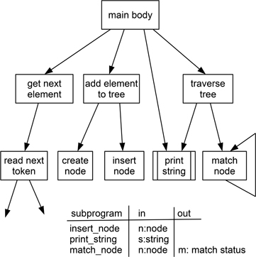
Figure 9.10: Simple illustration of a structure chart
Layout conventions help visualise structure, although they can get tricky with larger trees. The conventions used here include the following.
Sub-programs are grouped on levels, and each one is drawn below the level of the lowest calling unit. In the example, print_string() is drawn at the lowest level, because it is called from both main() and also traverse_tree(), which is on a level below main().
Double bars at the sides of a box (using print_string() as the example again) indicates where the designer is intending to use a standard ‘library’ component.
The use of recursion can be indicated by a closed invocation arc, as in the example of match_node.
While there may be no explicit convention about left to right ordering of sub-programs, there may well be an implicit one. Structure charts are often drawn with input activities on the left, and output activities on the right, which probably does help with understanding of a diagram.
Because the structure chart describes an invocation hierarchy, it is implicitly hierarchical in form, and so in principle at least, any box in the diagram could be expanded using the same form. However, for moderate-sized applications at least, this is normally only likely to occur for the lowest level, as shown here for read_next_token().
That said, given that some sub-programs are present purely for ‘house-keeping’ roles such as initialisation, rather than playing a role in the main function of the process, it may be useful to simply abstract the description of these as a single box (perhaps labelled as ‘initialisation activities’), particularly as they will usually only be invoked when the process starts. Doing so makes it possible to concentrate on those sub-programs that are involved with the main purpose of the application.
The structure chart does provide a relatively low level of abstraction from the final implementation of a solution. Because of this, tools do exist for reverse engineering such diagrams from code, so providing a useful tool for the maintainer. However, such tools will not readily ‘group’ sub-programs that are involved in performing a specific task, so layout may present a problem when analysing large applications with many sub-programs.
9.6Empirical knowledge about modelling processes
There are few empirical studies that explicitly address topics related to the modelling of single-thread processes, and the notations employed for this. Some studies do compare forms like the ERD with object-oriented notations (usually favouring the ERD notation) and these are discussed in the next chapter. Indeed, ERDs, and the different notations used for them, have formed the basis for comparative studies such as that described in (Purchase,Welland, McGill & Colpoys 2004).
One paper of relevance here is that by Moody (2009) which examines visual notations used in software engineering. One observation from this paper is that “most SE notations use a perceptually limited repertoire of shapes”. The De Marco form of DFD we examined in Section 9.2 is cited as an example of design excellence from this perspective. There is also some discussion of the ‘Principle of Cognitive Integration’, which relates to bringing together information from different diagrams (both diagrams of the same form and also diagrams of different forms). Interestingly, DFDs again demonstrate some good properties here, unlike the notations associated with the UML that we discuss in the next chapter.
Indeed, Moody's observation that “SE visual notations are currently designed without explicit design rationale” and that some older notations are “better designed than more recent ones” is a rather telling comment on the set of diagrammatical notations that together form a major design tool for software engineering.
Key take-home points about modelling processes
Modelling the attributes of processes uses a range of different forms to address the main viewpoints for each type of design element.
Design models. Modelling of single-thread processes largely uses notations that describe the functional and constructional viewpoints, although these can usefully be augmented by behavioural and data modelling notations. However, the latter are used in a supplementary role, being essentially unsuited to developing complete models.
Notational forms. While the DFD (in the De Marco format) makes good use of visual discrimination between different types of element, other notations tend to mainly use boxes and are dependent upon supplementary textual information.
Model integration. There is little scope to integrate design model information across the notations representing different viewpoints.
Tabular notations. While diagrams offer visual expressiveness, they have limited ability to handle large-scale cognitive issues. For some notations this may be aided by having a format that makes it possible to utilise hierarchy of diagram elements, but where this is lacking (as in the example of STDs) it may be useful to employ a tabular form to describe relationships in the model. Tabular forms also provide good support for checking a model for completeness and consistency.