In the previous chapter, I temporarily set aside a small and curious set of dynamical models of communities, most of which have not received the attention they deserve from mainstream theoretical community ecology. I have chosen to discuss them separately because I believe they are closer to the right track for developing a successful dynamical theory of biodiversity and relative species abundance. These models differ from the models discussed in the last chapter in that they explicitly incorporate the demographic processes of birth, death and dispersal.
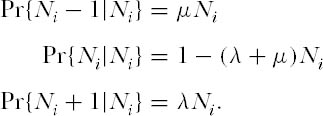
In the mid-1970s, when most eyes were still focused on the classical, niche-based theory of community ecology, Caswell (1976) made a bold attempt to create a neutral theory of community organization. Borrowing mathematical machinery from the theory of neutral evolution in population genetics, Caswell erected three models, only the first of which will be discussed here. In model I, communities are essentially collections of completely noninteracting species in which each species undergoes an independent random walk in abundance. Therefore, the total size of the community fluctuates. New species enter the community as a Poisson process (i.e., a rare event) with probability ν per unit time. This immigration probability, as in the theory of island biogeography, is independent of the identity of the species and of the number and identities of the species already present, except that only species not currently present are allowed to immigrate. This is equivalent to assuming that immigration makes a negligible contribution to the population dynamics of a species already present. Each new immigrant species becomes the founder of a line of descendants. Caswell assumed a linear birth-death process in which the stochastic per capita birth and death rates, λ and µ, are assumed to be equal, corresponding to the deterministic case of an intrinsic rate of increase, r, of zero. In other words, each species population is as likely to increase as it is to decrease per unit time. This is a pure drift process or random walk. The transition probabilities from a population of size Ni to size Ni − 1, Ni, or Ni + 1 at time t + dt are linear functions Ni of at time t, as follows:
Note in this model that λ and µ must be chosen to be sufficiently small that the expression (λ + µ)Nt < 1.
Caswell’s models II and III are similar to model I except that, instead of a constantly fluctuating community size, community size is held constant. The addition of constancy in community size is crucially important, and its absence is one of the major weaknesses of Caswell’s model I. Unlike the neutralists in population genetics, Caswell did not defend his neutral model as a realistic description of actual community dynamics. Caswell’s purpose in creating these models was to provide a neutral benchmark for comparison with the structure and dynamics of actual ecological communities. He developed a series of deviation statistics to measure departures of real communities from the predictions of his neutral models.
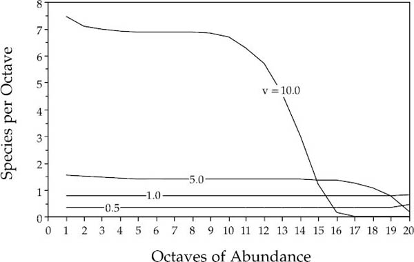
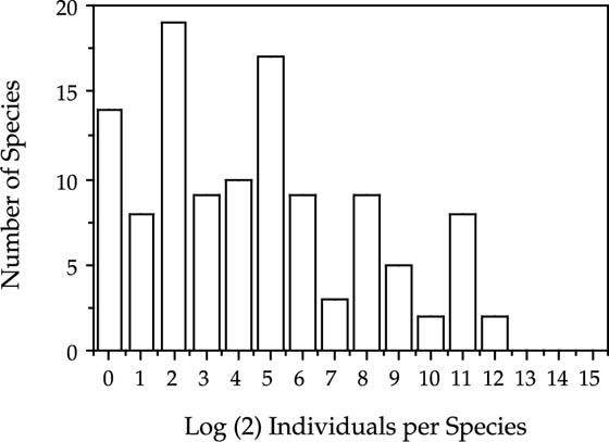
In any case, Caswell’s neutral results differ substantially from observed community relative abundance patterns. The relative abundance distribution predicted by Caswell’s model I is decidedly not lognormal on a Preston plot of octaves of abundance (fig. 3.1). Regardless of parameter values, the distributions tend to be nearly log uniform across many octaves of abundance. Only when the immigration rate was extremely high was there a even a hint of a log-normal like right-hand tail for the commonest species. The distributions also give no indication of having an interior mode at intermediate abundances. In fact, the distributions are closer to the logseries of Fisher et al. (1943) than they are to the lognormal (Caswell 1976), but the logseries is not a particularly good fit, either.
FIG. 3.1. Relative abundances predicted by Caswell’s neutral models are decidedly not lognornal-like. The family of curves in the figure is drawn for various rates of new species addition to the community (parameter v) per unit time. The distributions are extremely flat across many octaves fo abundance. Only when the immigration rate is very high does the distribution develop a right-hand tail. Moreover, these distributions are transient because the number of species in the models increases with time without bound.
However, there are much more serious problems with Caswell’s model. One is that the size of the community grows without bound over time. Community size, J, where J is the total number of individuals in the community, is a negative binomial random variable with mean E{J} = t → ∞ (elapsed time), and variance as Var{J} = t(t + 1) → ∞ as t → ∞. A second major problem is that the expected number of species in the community, E{S}, is linearly proportional to the colonization rate of new species per unit time, ν, and the log of elapsed time:
E{S} = Var{S} = v · ln(t + 1).
I think it is safe to assume that no one would accept these results as reasonable for real ecological communities.
Given the unreasonableness of Caswell’s model, it is logical to ask, why pay so much attention to it? To my knowledge, Caswell was the first person to recognize the importance of basing a model of relative species abundance explicitly on birth, death, and dispersal processes. Moreover, as will shortly become apparent, with the addition of the biologically reasonable assumption of a finite community size and minor changes in the birth, death, and dispersal processes, a much better model is obtained. Indeed, it is unclear why Caswell’s models II and III, which had a constant community size, didn’t perform better than his model I. Caswell (1976) asserts that the results from all three models were qualitatively similar, but he did not actually report on the behavior of models II and III in his paper.
The importance of a finite community size cannot be overemphasized. Ecologists who work on space-limited communities seem generally more aware of this fact than others. For example, plant ecologists who study sessile plants, and marine ecologists who study intertidal or benthic invertebrate communities, recognize that there is an unavoidable physical constraint on the total number of individuals that can be packed into a given space (Hughes 1984, 1986, Yodzis 1986, Weiner 1985, Jackson et al. 1996, Harper 1977). Space per se of course is not a resource, but it is a good surrogate variable for limiting resources that are distributed uniformly over the two-dimensional landscape, such as sunlight or planktonic food. When access to resources requires controlling a unit of space, it is reasonable to refer to space as a limiting resource. It should be noted, however, that even when space is not the limiting factor, limiting resource availability per unit area will ultimately impose a finite limit on the density of competing organisms within a given ecological community in a defined space (Brown 1995). Across communities of trophically dissimilar species, densities of organisms per unit area will vary, depending on the relative sizes and energy demands of species in the different communities. However, within a given community of trophically similar, competing species, the numbers of organisms per unit area should not vary too widely (i.e., by orders of magnitude) from one locale to the next.
Preston (1948) was fully aware of this fact, as were MacArthur and Wilson (1967), who noted that the total number of individuals in a defined taxon or community, J, increases linearly with the area, A, inventoried:
J = ρA,
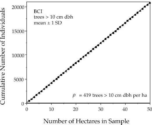
where ρ is the density of individual organisms per unit area. Figure 3.2 illustrates this relationship for an enumeration of trees in a closed-canopy tropical forest on Barro Colorado Island (BCI), Panama, in a 50 ha plot of mixed, species-rich, old-growth forest. The plot has been completely censused five times for all free-standing woody stems >1 cm diameter at breast height (dbh) (Hubbell and Foster 1983, 1990). This relationship holds very precisely (r2 ≈ 1.000) over more than five orders of magnitude of variation in area, from 1 m2 to 5 · 105 m2 (the largest area censused). It holds despite the fact that more than three hundred species occur in the BCI plot, that the species composition of the BCI plot varies greatly from place to place, and that relative abundances of species range over more than four orders of magnitude (1 to over 40,000).
FIG. 3.2. The individuals-area curve for a 50 ha plot of tropical moist forest on Barro Colorado Island, Panama. The plot is of individuals with a trunk diameter >10 cm dbh of all species. The curve represents the mean of one hundred random starting points for accumulation of area within the plot. The linearity is very precise. One standard deviation about each mean is also plotted, but they are so small that they are barely visible. The mean density of individuals >10 cm dbh per hectare, ρ, is 419 trees.
We can state this as an important general principle, namely, that large landscapes are essentially always biotically saturated with individuals of a specified metacommunity or taxon. No significant amount of space or other limiting resource goes unused for long. Small areas or patches of resource may become unsaturated for short periods of time immediately after disturbances, but at large landscape scales, the surface of the earth, to a first approximation, is completely and permanently saturated. In fact, if landscapes were not more or less continuously saturated with individuals, such a simple, linear relationship would not be found.
One could imagine all sorts of possible causes of variation in the density of individuals. A failure to obey this principle would suggest at least three possible conclusions. The disturbance regime could be so severe on landscape scales that the region is not, in fact, saturated, and permanent open space or unused limiting resource exists. Or there could be variation over the landscape in the overall regional supply rates of limiting resources for the community as a whole (landscape variation in potential productivity). Or one might be attempting to aggregate taxa that are trophically too dissimilar to be logically treated as members of the same metacommunity (chapter 1). Or all three possibilities could be true simultaneously. The remarkable fact is, however, that a linear relationship between the number of individuals in a well-characterized community and area is almost universally observed, at least on relatively homogeneous landscapes.
The implications of this simple—indeed, seemingly trivial—relationship between individuals and area are far more profound than at first apparent. At least two major theorems about biogeography and relative species abundance follow from this first principle. The first theorem follows immediately, namely, that the dynamics of ecological communities are a zero-sum game. If, as the relationship implies, the density of individuals ρ is a constant, then any increase in one species must be accompanied by a matching decrease in the collective number of all other species in the community. The sum of all changes in abundance is always zero. Thus, the total number of individuals in the community behaves like a conserved quantity, except that individuals of one species cannot be transmuted into individuals of another species (speciation excepted). Unlike subatomic particles, however, individuals can reproduce themselves. This reproductive property fuels a birth process that replaces individuals that die in the community in a zero-sum game. When one species is successful at reproducing beyond self-replacement, other species must have compensatory failures in reproduction. No new individuals can be added to an ecological landscape by birth or immigration until vacancies have been created by deaths. Note that the zero-sum game does not actually require that the carrying capacity of the landscape be constant through time or space; it only requires that the landscape be biotically saturated at all times, i.e., that the biota fully track changes in limiting resources.
The second important theorem that follows from the biotic saturation of landscapes and the zero-sum dynamics of ecological communities is not immediately obvious, however, and is essentially the subject of the remainder of this book. This theorem concerns the consequences of zero-sum dynamics for the equilibrium distribution of relative species abundance in local communities and in the metacommunity, given certain rules of the zero-sum game. This theorem is the subject of formal proofs in chapters 4 and 5, but I anticipate some of the results qualitatively in this chapter.
The rules of the zero-sum game now have to be considered. How the game is played could be anything—so long as the sum of all abundance changes is zero. For example, rare species might have a per capita competitive advantage (frequency dependence), and/or per capita population growth rates may decline with increasing population size (density dependence). The question now arises, what rules do zero-sum community dynamics have to obey to result in a lognormal-like distribution of relative species abundances? The answer to this question is the second theorem to follow from our first principle, and will only finally and fully be answered in the next two chapters.
The next steps in answering this question were taken by me (Hubbell 1979), working on closed-canopy, tropical forests, and by Hughes (1984), working on benthic marine invertebrate systems, both space-limited communities. Hughes and I independently developed stochastic models of relative species abundance that were similar in certain important respects. Both models explicitly assumed zero-sum community dynamics, and both specifically modeled birth and death processes. Because Hughes’s model is considerably more complex and specific than mine, however, I will not discuss his model further.
I began with the simplest possible assumption of a community obeying zero-sum dynamical rules that were neither frequency nor density dependent (except for fixed community size). Consider a model community that has J total individuals, regardless of species, so that our first principle applies and the community obeys zero-sum dynamics. Each individual occupies one space or unit of limiting resources and resists displacement by any other individual. Eventually, however, the individual dies, with probability µ per unit time, and it is replaced by a “birth.” Now suppose that the replacing species is randomly drawn from the community. Let the probability that the replacing individual is of species i be given by the current relative abundance of species i. Let the current abundance of species i be Ni. Then, the transition probabilities that species i will decrease by one individual remain unchanged in abundance, or increase by one individual during one time step are given by
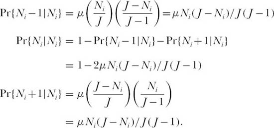
Thus, the probability that species i will increase by one individual is the probability that a death occurs in a species other than species i, or µ(J − Ni)/J times the probability that the next birth occurs in species i, or Ni/(J − 1). Note that the probabilities that species i will increase or decrease are identical. This model is even simpler if we scale time so that a single time step is the mean time required for one death to occur (µ = 1).
Species in this simple neutral model are identical and equal competitors on a per capita basis. They have identical per capita chances of dying and of reproducing. Each species has an average stochastic rate of increase, r, of zero. The dynamics of the model community is therefore a random walk. For this reason, I call this process ecological drift in analogy with genetic drift. Unlike Caswell’s (1976) neutral model I, however, this random walk is not completely free and unfettered. The random walk is constrained by the fact that all species abundances must sum to a constant J, i.e., the sum of all positive and negative changes in abundance must sum to zero. J can be large or small depending on the density of individuals, ρ, and the size of the area occupied by the community. No species in the community can increase in abundance above the absolute maximum imposed by J, which corresponds to complete dominance. Conversely, a species can decline to zero abundance, an absorbing state that corresponds to local extinction. However, the ecological drift of a species to extinction can be quite a long process, as will be discussed in chapter 4.
I return now to the central question, namely, what rules must the zero-sum dynamics of ecological drift obey in order to obtain a lognormal-like distribution of relative species abundances? It turns out that the rules of the zero-sum game are indeed critical to the answer. As will be fully explored in the next two chapters, the answer is this: Relative species abundances are lognormal-like if community dynamics obey a zero-sum random drift process. This is the second theorem that follows from our first principle under zero-sum ecological drift. An even more remarkable result, which presently is still a simulation-based mathematical conjecture, is that lognormal-like distributions of relative species abundance are not obtained when the rules of the zero-sum game are density or frequency dependent. I will discuss the evidence for this conjecture shortly.
I use the term lognormal-like because the theoretical distribution of relative species abundance predicted to occur in local communities by the unified theory (chapter 5) is not a lognormal (Hubbell 1995). I have named this new statistical distribution the zero-sum multinomial (Hubbell 1997). The zero-sum multinomial distribution is discrete, not continuous. In many cases, however, casual inspection will not be able to distinguish a zero-sum multinomial from a log-normal when the latter is approximated by a discrete-valued function (e.g., a Preston curve). It also differs from a log-normal in having a long, attenuated tail of rare species (see chapter 5), so that the distribution is asymmetrical about the modal octave. Otherwise, the distributions are very similar, particularly in octaves to the right of the mode. Bell (2000) used simulations to explore some properties of the distribution as community size and immigration rate are varied, a topic to which I shall return in chapter 5. The distribution has similar sampling properties to Preston’s lognormal distribution in that, as sample size is increased, more and more of the zero-sum multinomial is revealed. Only when sample sizes are large will the differences between the zero-sum multinomial and the lognormal become clear in the long tail of very rare species. Also, under one of the two modes of speciation studied in this book, a different distribution of relative species abundance is predicted for the metacommunity than for the local community, as we shall see in chapter 8.
It is easy to understand qualitatively why relative abundances would tend to be lognormal-like rather than normal-like under neutral zero-sum ecological drift. In the drifting community, there are many approximately normally distributed fluctuations of species about their current respective abundances. But common species will tend to fluctuate more in absolute abundance because they undergo absolutely more births and deaths per unit time than rare species. This will be true even though on a per capita basis, birth and death probabilities are the same in all species. However, the critical factor is that these species fluctuations collectively must obey the zero-sum rule. Having zero-sum ecological drift in essence multiplicatively couples the fluctuations among species. This coupling produces the lognormal-like distribution of relative species abundance observed when species frequency is plotted against arithmetic individuals per species.
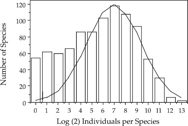
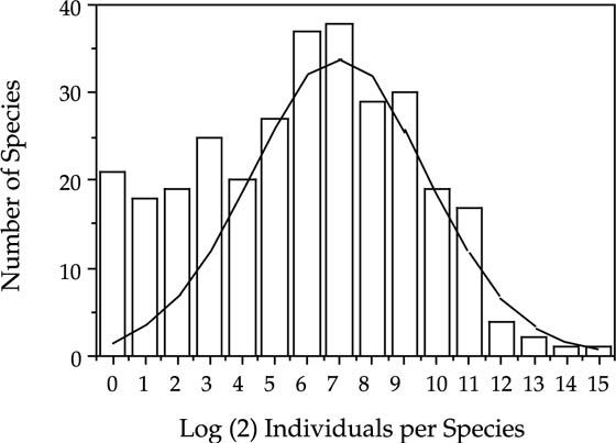
The dependence of lognormal-like relative species abundances on zero-sum ecological drift is illustrated by the contrasting relative abundance patterns of tree species in three tropical forests. Each of the communities were sampled by 50 ha permanent plots. Two of the communities, Pasoh and BCI, are closed-canopy forests in which zero-sum dynamics operate. The relative species abundance distributions for Pasoh (fig. 3.3) and BCI (fig. 3.4) are lognormal-like. They are remarkably similar in their variance and in their modal octave of species abundances, despite the fact that they have very different taxonomic compositions and evolutionary histories. The main difference is that the Pasoh plot has about two and a half times as many species as the BCI plot. The third tree community is located in Mudumalai Game Reserve in the Western Ghats of southern India. Mudumalai is an open-canopied forest with a grass-dominated understory and less than 25% total tree cover (R. Sukumar, pers. comm.). In contrast to Pasoh and BCI, the open-canopied forest at Mudumalai has a distribution of relative species abundance that is decidedly not lognormal-like (fig. 3.5). The unified theory explains this observation by the fact that the canopy of the Mudumalai forest is not saturated with trees. Therefore, the population dynamics of individual tree species are to a large extent independent of one another, and are not constrained to follow zero-sum dynamics like populations of tree species in the closed-canopy Pasoh and BCI forests.
FIG. 3.3. Lognormal-like distribution of the relative abundances of the tree species in the 50 ha plot in a closed-canopy forest in Pasoh Forest Reserve, Peninsular Malaysia. The best-fit lognormal is superimposed on a Preston plot of species frequencies per octave of abundance. Compare with the plot for the 50 ha plot on Barro Colorado Island, Panama (fig. 3.4). Note the poor fit to the rare species. This deviation in having too many rare species is another almost universal pattern in closed-canopy forests, about which more will be said later (see also fig. 3.4). Data from Manokaran et al. (1993). The graph represents counts of all stems >1 cm dbh. The zero-sum multinomial will be fit to the full curve in chapter 5.
Recall that Preston (1962) claimed to have found a canonical relationship among the parameters of the lognormals that seemed to characterize many ecological communities. If J/nr—the ratio of all individuals to the number of individuals of the rarest species in the community—was specified, then Preston argued that all of the other parameters of the lognormal could be deduced. Note that J/nr can be rewritten in terms of area as ρA/nr. In finite samples, nr will usually be unity, which is the smallest observable abundance. Therefore, if Preston’s empirical generalization were correct, then the canonical lognormal and the relaive species abundance distribution itself should be completely characterizable from the mean density of individuals per unit area, and the total area sampled. This is clearly false. MacArthur and Wilson (1967) did not remark on this prediction, but they did argue that the canonical lognormal predicted a quantitative species-area relationship, specifically a log-log linear relationship between the log of the number of species S and the log of J/nr. At intermediate regional spatial scales, this is true (May 1975), but, as I shall show in chapter 6, it is decidedly not true on local spatial scales. I shall also show that the metacommunity distribution of relative species abundance cannot be completely determined by the mean density of individuals and the total area sampled. The critical missing parametric ingredients are the rates of speciation and dispersal (see chapter 6).
FIG. 3.4. Lognormal-like distribution of the relative abundances of tree species in the 50 ha plot in a closed-canopy forest on Barro Colorado Island, Panama. The best-fit lognormal is superimposed on a Preston plot of species frequencies per octave of abundance. Compare with the plot for the 50 ha plot in Pasoh Forest Reserve, Peninsular Malaysia (fig. 3.3). Note the poor fit to the rare species. This deviation in having too many rare species is another almost universal pattern in closed-canopy forests, about which more will be said later chapter 5 (see also fig. 3.3). The graph represents counts of all stems >1 cm dbh. The zero-sum multinomial will be fit to the full curve in chapter 5.
FIG. 3.5. Nonlognormal-like distributions of the relative abundances of tree species in the 50 ha plot in open-canopy woodland in Mudumalai Game Reserve, Western Ghats, India. This is a forest that has a thick grass understory that burns in most years. The forest is also disturbed by elephants. The graph represents counts of all stems >1 cm dbh. Data courtesy of R. Sukumar.
The relative abundance distributions predicted by the zero-sum multinomial are only accidentally and occasionally canonical sensu Preston (1962). This is perfectly all right, in my opinion, because it is easy to show that the canonical relationship is neither a mathematical nor an empirical necessity, and indeed that it cannot be generally true. Canonical lognormals have typically been observed in communities having relatively small numbers of species and high variance in relative species abundance, or in cases of small sample sizes that have not unveiled the rarest species. Most of Sugihara’s (1980) example communities that exhibited canonical distributions were relatively species poor. On the other hand, species-rich communities in which the commonest species comprise only a small percentage of total individuals often do not exhibit canonical lognormals. For example, the lognormal-like distributions of relative tree species abundance in the Pasoh and BCI forests are not canonical. These distributions exhibit large excesses of rare species over the number predicted by the lognormal (figs. 3.3 and 3.4). Moreover, the modes of the Individuals Curves for Pasoh or BCI are not located in the ultimate octave of the Species Curve.
Preston (1980) himself later acknowledged finding communities with noncanonical lognormal relative species abundance patterns. In fact, it has to be the case that all “true” distributions of relative species abundance in nature are not canonical, a fact that will be revealed if and when they are adequately sampled. If relative abundance lognormals were always canonical, then from the logic of the putatively canonical species-area relationship given above, there should be one and only one possible number of species S in communities of density ρ and area A. In fact, the number of species in real communities occupying a fixed area is observed to vary considerably, from monodominant communities to species-rich communities—even though the total number of individuals in the fixed area does not vary greatly. Factors affecting S in a particular area (e.g., an island) include birth, death, and immigration rates—among the basic ingredients of MacArthur and Wilson’s theory of island biogeography.
The breakdown of the canonical relationship occurs primarily because of the long asymmetrical tail of rare species in real communities. Suppose species relative abundances were truly lognormal and the number of species, S, in the community were fixed as Preston claims. Then, in principle, one should be able to increase sample sizes sufficiently that the last and rarest species would have abundances greater than unity. This is because, in Preston’s universe, the number of species is finite, so that if a sufficiently large sample is taken, they will all be found. In order for the lognormal to be canonical, the number of octaves separating the rarest species from the commonest species must remain constant. Therefore, as the common species become commoner with increased sample size, the rarest species must also become commoner. However, in real samples, the abundance of the rarest species sampled, nr, almost invariably remains “locked” at unity. Thus, there is no fixed relationship between the total number of individuals in the community, J, and the abundance of the rarest species, nr. As sample size increases, new rare species never before sampled are added ever more slowly, and the rarest species become ever rarer relative to common species in a seemingly endless regression. This means that the number of octaves of abundance separating the rarest species from the commonest species grows steadily greater. This sampling phenomenon is observed and is predicted by the present unified theory, but not by Preston’s canonical lognormal hypothesis.
In reference to immigration, in island biogeography theory the number of species at equilibrium on an island is sustained only under a persistent rain of immigrants. There are parallels in the theory of ecological drift. Under drift without immigration, species will gradually be lost from the community because of local extinction. However, because the landscape remains saturated with individuals, the mean abundance of the surviving species must thereby increase. The elimination of species under ecological drift can be very slow, especially for large communities (chapter 4). Without immigration, the community eventually collapses to a single species in a final equilibrium. However, with immigration (or speciation), a persistent multispecies equilibrium community is achieved with a distribution of relative species abundances that is determined by community size J and the probability of immigration into the community. In these multispecies, multinomial equilibria, the number of species is not a free parameter as it was in the static, niche-assembly theories of relative species abundance discussed earlier (chapter 2). Instead, both the equilibrium number of species as well as their equilibrium relative abundances are predictions of the unified theory.
The next dynamical model I wish to consider is quite famous. It is the lottery model of Chesson and Warner (1981) and Chesson (1986). This model of community dynamics differs from the ecological drift model in having a frequency-dependent birth process. Rare species in Chesson and Warner’s model community enjoy a per capita advantage in reproduction over common species. The lottery model, originally proposed by marine ecologist Peter Sale (1977, 1980) for space-limited communities of coral reef fish, assumes that space is allocated at random or by “lottery,” and it is one specific case of what Chesson and Warner called the “storage hypothesis.” Because of recruitment fluctuations, rare species accrue an advantage in winning vacated space.
Chesson and Warner’s model of community dynamics is as follows. Let Ni(t) be the population of adults of the ith species at time t. Then the number of the ith species present one time step later is given by
Ni (t + 1) = (1 − µi) Ni (t) + Ri (t) Ni (t)
where µi is the adult death rate and Ri(t) is the time-varying, per capita recruitment rate of new adults into the population. Chesson and Warner suggest that a great number of varying environmental factors could influence Ri(t). They called the model the “storage hypothesis” because recruitment fluctuations only promote frequency-dependent coexistence if adults live for more than a single reproductive season, i.e., there are overlapping generations. The average lifespan is the inverse of the adult mortality rate, or  . Therefore, there are overlapping generations if µi < 1.
In the lottery case, the relative recruitment rate for species i at time t is simply the number of spaces vacated by deaths at time t multiplied by the fraction of all births in the community that are of species i. The total number of deaths in the community at time t is ΣkµkNk. If λi(t) is the per capita birth rate of species i at time t, then Ri(t) is
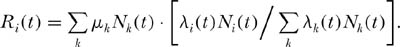
Note that if in a given time period species i is the only species reproducing, then λi(t)Ni(t)/Σk λk(t)Nk(t) is unity, and all the vacant sites are won by species i in that time period. Note also that this birth or recruitment function is identical to the drift model that forms the basis of the unified theory if the λ’s are constant and unity. In fact, except for rare species recruitment advantage, the lottery version of Chesson and Warner’s model is virtually identical to ecological drift. It differs in having a deterministic death process; but most importantly, it has the same zero-sum dynamics. Species are identical competitors in the following sense: if any species becomes rare, that species will enjoy the same frequency-dependent reproductive advantage as any other equally rare species, and all suffer the same frequency-dependent disadvantage if they become common.
The result that made Chesson and Warner’s model famous was their proof that variability per se could promote coexistence. Prior to their analysis, the conventional wisdom was that variability was just noise that would have no effect on, or even reduce the possibility of, coexistence. For example, Turelli (1978a,b) and Turelli and Gilpin (1980) studied Lotka-Volterra competition equations with stochastic variation in carrying capacities, competition coefficients, and intrinsic rates of increase, but found essentially no effect on coexistence. However, Chesson and Warner showed that temporal variation in the birth process, but not in the death process, could allow two competitors, or n competitors, to coexist under conditions that would otherwise lead to competitive exclusion under constant recruitment.
A simple hypothetical example told to me by Bob Warner illustrates the basic principle. Imagine a model reef fish community of two interspecifically territorial fish. One species is common and its adults currently occupy 90 of the 100 territories on the reef. The other species is rare and its adults occupy the remaining 10 territories. Now suppose that there is 10% annual adult mortality, and it is random across the two species. Then nine deaths are expected in the common species, but only one death in the rare species. If each species reproduces annually in proportion to their adult abundance, then the only changes in abundance that will occur will be due to random drift. However, if there is a tendency for the rare species to reproduce in years when the common species does not, then coexistence will occur. This is because of very strong rare-species advantage. In this numerical example, if the rare species occupies all of the vacated territories in a given year, its population will increase by 90%, whereas the common species will have decreased by only 10%. Chesson and Warner (1981) prove that all that is required for coexistence is that there be overlapping generations and some temporal variability in recruitment rate; recruitment does not have to be completely asynchronous.
Chesson (1986) noted that the frequency dependence in the model is strong enough to bound each species away from zero abundance so that coexistence will occur. However, one might argue that the frequency dependence is overly and unrealistically strong. For example, according to their model, a very rare species reduced to a single individual in a very large community can potentially produce enough offspring to win every vacant site. The larger the community, the more sites that are vacated per unit time, and the rarer a species is, the stronger the rebound-from-rarity effect becomes in their model. There is essentially no upper bound to the strength of frequency dependence in Chesson and Warner’s model. In actual communities, on the other hand, dispersal limitation (Tilman 1994, Hurtt and Pacala 1995) and biological constraints on individual fecundity will set finite limits on maximum per capita recruitment success. I suspect that the realized recruitment success of most rare species will be far lower than in Chesson and Warner’s model. Whatever frequency dependence rare species enjoy will often not successfully bound rare species away from zero abundance. And this must be so, because otherwise no species would ever go extinct, locally or globally.
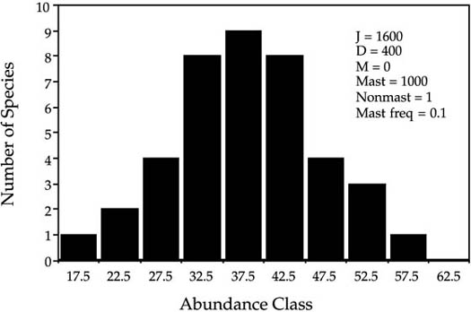
More germane to the present discussion, however, are the implications of Chesson and Warner’s model for relative species abundance. It is surprising, but this question has apparently never been asked. Without waiting for analytical results, which may be very difficult to obtain in any event, one can easily simulate the dynamics of a model community with frequency dependence in the recruitment process. I simulated tree communities of varying numbers of masting tree species. Tree species that mast—for example, the oaks in eastern North America, or the dipterocarps of Southeast Asia—are species that flower and fruit on variable intervals of several years (Curran et al. 1999). In many masting species, there is interspecific synchrony in masting years, presumably to reduce collective seed and seedling predation (Janzen 1974). In my simulations I modeled forests in which masting behavior was simply stochastic, occurring with probability ξ per year. The results were that, regardless of the value of ξ or the size of the mast, or the number of species in the community, the outcome was always coexistence, just as predicted by Chesson and Warner. However, the stochastic equilibrium relative species abundances were never lognormal-like. A typical example of the distribution of individuals per species from one of the simulations is presented in figure 3.6. In this figure, the abundance classes are plotted arithmetically, not log transformed, so it is easy to see that relative species abundances are very close to being perfectly normally distributed.
FIG. 3.6. Plot of the distribution of relative species abundance predicted by the lottery model of Chesson and Warner. Note that the histogram is of arithmetic abundance, not logarithmic abundance. The non-lognormality of the curve is apparent.
I have explored a number of other models of density and frequency dependence in addition to the lottery model, and the result has always been qualitatively the same under zero-sum ecological drift. The distribution of the number of individuals per species is never lognormal (or zero-sum multinomial). For example, one can study community dynamics and relative species abundance under stochastic logistic growth. Consider a case in which all species had a maximum carrying capacity of J (community size). Let the per capita birth and death rates, λ and µ, be the standard logistic expressions λ(Ni) = 1 − bNi and µ(Ni) = dNi, where slopes b and d are chosen so that J = (b + d)−1. The probability that species i will increase by one individual in one time step is therefore λNi/ Σk λ(Nk), and the probability that species i will decrease by one individual is µNi/ Σk µ (Nk).
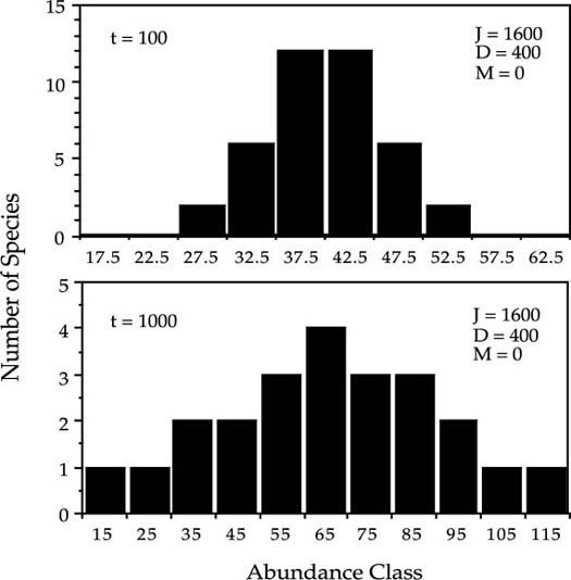
FIG. 3.7. Nearly normal transient distributions of relative species abundance for a community obeying zero-sum dynamics, in which each species grows according to a stochastic logistic, each with an identical carrying capacity of the community size, J. Species are only very slowly lost to extinction because of the density dependence. Note that the abundance classes are arithmetic, not logarithmic. Numbers of species represent the mean number of species in abundance classes in one hundred runs of the model.
I illustrate the qualitative behavior of the stochastic logistic community model with the results of one simulation (fig. 3.7). In this case the community size J was set at 1600 with initial conditions of forty equally abundant species having forty individuals apiece. In each disturbance cycle, a quarter of all individuals died and were replaced according to the stochastic logistic. A quasi-equilibrium, near-normal distribution of relative species abundance is achieved quite rapidly. Figure 3.7, top panel, shows the abundance distribution after one hundred disturbances. It is a quasi-equilibrium because the community loses species to extinction very slowly. As species are gradually lost, the variance in relative species abundance increases but the distribution remains very nearly normally distributed. After one thousand disturbances, the distribution is still essentially normal, not lognormal-like (fig. 3.7, bottom).
In my simulations, the distributions of relative species abundance produced by these models are always closer to being normal than lognormal. On reflection, it is clear why this is so under zero-sum ecological drift. Frequency and density dependence that give rare species a competitive advantage will tend to make rare species relatively more common, and simultaneously make common species rarer. Frequency dependence compresses the tails of the distribution of species abundances, lessening the skewness of the distribution when it is plotted arithmetically. Density and frequency dependence act as centrally tending forces that reduce the variance in abundances of species in the community by driving them toward middling abundances. In contrast, under zero-sum, ecological drift, there are no such centrally tending forces. These results do not imply the converse, however, that in the absence of zero-sum ecological drift, one cannot obtain a lognormal-like distribution of relative species abundance. The last dynamical model I discuss makes this point.
The final model represents recent theoretical work by Engen and Lande (1996). Their results are important for several reasons in the present context. First, they show that one cannot conclude that density dependence is absent from a community simply by observing relative abundance distributions that are lognormal. Second, their model allows for both demographic and environmental stochasticity in the population growth rate. Thus, Engen and Lande’s model is in many ways very close to the present theory. They introduce a new class of stochastic species abundance models that includes a process of speciation and density dependence. Their paper is rather technical, however, and so only a general overview of their results are discussed here. For more detail, the reader should consult their paper.
Engen and Lande assume that new species originate slowly by a Poisson process that can be inhomogeneous in the sense that species do not have to have the same speciation rate. They study the stochastic changes in abundance of an arbitrary species by assuming that small changes can be modeled by a diffusion approximation. Let the current abundance of such a species be x, and let the stochastic distribution of abundance be λ(x). For simplicity, assume that the speciation rate is constant (ω0). They then show that the mean amount of time that a species undergoing stochastic population fluctuations spends at abundances between x and x + ∂x is given by
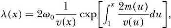
where m (x) and v (x) are the infinitesimal mean and variance of abundance. Now, let us suppose that population growth is density dependent. Consider the following general differential equation for density-dependent growth:
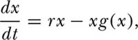
where r is the intrinsic rate of increase of the population. The density-dependent function g(x) can be anything, but a well-known function is the Gompertz, where g(x) = γ log(x) (they actually use a form of density dependence that is very close to but not exactly the Gompertz in order to get a closed integral solution). The per capita growth rate of the populations falls off linearly with the logarithm of abundance. Now, to make the growth equation stochastic, let the intrinsic rate of increase r have both an environmental variance  and a demographic variance
 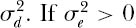 , then the distribution of abundance is given by
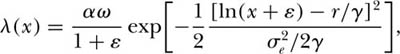
where
and
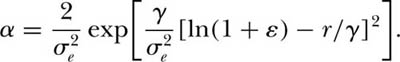
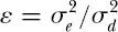
This equation for λ(x) is a lognormal model shifted or translated from x to x + ε, where ε is the ratio of environmental to demographic stochastic variance.
Engen and Lande’s (1996) model differs in a number of important ways from the neutral model developed in this book. First, it treats the effects of both environmental stochasticity and demographic stochasticity on population dynamics, whereas the theory I develop here thus far only has demographic stochasticity. Second, it incorporates density-dependent population growth without zero-sum dynamics. The theory here assumes zero-sum dynamics that cap maximum population size, but it does not impose per capita restraints on birth and death rates that change with population size. Thus far, their theory does not include migration rates, whereas the present theory does (chapters 4–6). It should be possible to evaluate which theory applies in a particular situation by the relationship between the mean and variance of population sizes across a community. More importantly, although Engen and Lande’s theory can produce a lognormal relative abundance distribution with the appropriate choice of model for stochastic density dependence, we have seen that most observed relative abundance distributions are not, in fact, lognormal. It remains to be seen whether their model can produce the asymmetrical zero-sum multinomial distribution of relative species abundance with its observed long tail of very rare species. I now turn my attention to the development of the unified neutral theory of biodiversity and biogeography.
1. Relatively few models have taken a dynamic approach to a theory of relative species abundance, building on processes of birth, death, migration, and speciation. The first of these dynamical theories, by Caswell, would have performed far better had the assumption of constant community size and zero-sum dynamics been explored.
2. The key first principle of the unified neutral theory is that the dynamics of communities are a zero-sum game. No species can increase in abundance in the community without a matching decrease in the collective abundance of all other species.
3. This principle follows immediately from the generally observed, remarkably precise, linear relationship between the number of individuals and sample area in a community, a relationship that holds quite generally in ecological communities, irrespective of the turnover of species from one local area to another.
4. If the dynamics of species abundances are neutral on a per capita basis under zero sum dynamics, then a theorem can be proven about relative species abundance that predicts that relative abundances will be described by a new statistical distribution called a zero-sum multinomial.
5. The zero-sum multinomial distribution is similar to a lognormal distribution for common species, but it differs in shape for the rare species. Unlike the lognormal, it is asymmetrical, typically with a long tail of very rare species. Most newer, larger datasets on relative species abundance in natural communities exhibit this asymmetry and long tail of rare species.
6. The long tail of very rare species means that relative abundance distributions are not canonical, sensu Preston, because there is no fixed relationship between the total number of individuals sampled and the abundance of the rarest species.
7. At least one other dynamical theory of relative species abundance has, with different assumptions, been able to generate lognormal distributions. However, none of the other theories except the present one reproduces the zero-sum multinomial distribution and the long tail of rare species observed in real datasets.