The rate at which species accumulate with increasing area surveyed—the species-area relationship—is perhaps the most basic and fundamental problem in biogeography. Yet on first consideration, a positive species-area relationship appears to be little more than a trivial corollary of the principle that Earth and its limiting resources are permanently and completely saturated with organisms. In an infinitely diverse world (θ = ∞), the number of species would equal the number of individuals, and the number of species would therefore increase linearly with area. Short of infinite diversity, however, the biotic saturation of landscapes dictates that the number of species must accumulate more slowly than the number of individuals. The inevitability of a positive species-area relationship has led some ecologists to suggest that it is of little biological interest (e.g., Connor and McCoy 1979, Gilbert 1980, Connor et al. 1983). However, the species-area problem is far deeper than it might at first seem. One must explain why species-area relationships show strong and recurrent qualitative and quantitative patterns (Johnson and Raven 1973, Connor and Simberloff 1978, McGuinness 1984, Williamson 1988, Palmer and White 1994, Rosenzweig 1995). This chapter explores the unified theory’s explanations of these recurrent patterns.
A debate over the relationship between species number and area has persisted for a long time. This controversy has been partly prolonged by failure to recognize that the species-area relationship obeys different scaling rules on different spatial scales (Palmer and White 1994, Rosenzweig 1995). But it has also been controversial because there is no theoretical foundation for species-area curves that derives from fundamental processes of population dynamics. Like most contemporary theories of relative species abundance, most current theories of species-area relationships are static and ad hoc sampling hypotheses. MacArthur and Wilson (1967) discussed the lognormal in relation to species-area curves in the first chapter of their monograph. However, they never actually formally connected their dynamical theory of island biogeography to species-area relationships (Williamson 1988). Later, May (1975) analyzed the expected accumulation of species with increasing area under a variety of statistical distributions, including the broken stick, logseries, and the lognormal. This approach presupposes that what matters most to the species-area relationship is the sampling of local species abundance. It ignores not only community dynamics but also dispersal limitation. If species are dispersal limited, then the expected local relative abundances of species will not be the same as random samples of the metacommunity (chapter 5). All species are dispersal limited on some spatial scale, and dispersal limitation becomes increasingly important on larger scales.
In hindsight, however, May (1975) made the almost prescient observation that “if relatively small samples are taken from some large and homogeneous area, the relation between sample area (or volume), A, and the number of species represented in the sample, S(A), is likely to obey the logseries.” The unified theory’s explanation for this observation is that taking many scattered small samples will tend to overcome and compensate for dispersal limitation, and thus more closely approximate a random sample of the metacommunity with its nearly logseries equilibrium distribution of relative species abundance (chapter 5).
In previous chapters I have focused on the predictions of the neutral theory for patterns of species richness and relative abundance in the metacommunity and in local communities or on islands. However, the explicit linkage of the theory to biogeography on continuous landscapes has not yet been made because space has been treated implicitly. Indeed, the original theory of island biogeography did not treat space explicitly, either. Treating space implicitly is permissible when discussing migration from a mainland metacommunity to islands whose dynamics occur on very different spatial and temporal scales. But it is no longer acceptable in a general theory of biogeography on continuous landscapes—the theory needed to achieve deeper understanding of species-area relationships. Treating space explicitly also causes one very significant change in the neutral theory. Under explicit space, the metacommunity is no longer uniquely determined by the fundamental biodiversity number θ alone. It also becomes necessary to specify the mean rate of dispersal of individuals over the metacommunity landscape.
Some analytical progress on dynamical contact-process models of species-area relationships has recently been reported by Durrett and Levin (1996), and their results will be discussed shortly. But many questions about species-area relationships and the distribution of species diversity on continuous landscapes remain unsolved analytically. Fortunately, however, little is lost because the spatially explicit version of the unified theory is easily simulated in numerical experiments, and the analytical results of previous chapters provide a useful guide to interpreting the results of these simulations.
In this chapter I first discuss the theoretical species-individual sampling curve that arises in the metacommunity under the simplifying assumption of no dispersal limitation. This result leads to a neutral theoretical justification for Fisher’s α. To examine species-area relationships and spatial patterns of species diversity under dispersal limitation, I study a spatially explicit version of ecological drift. I analyze the dynamical behavior of a metacommunity landscape “tiled” with identically sized local communities that exchange migrants with neighboring communities. I then discuss the steady-state species-area relationships that arise on this landscape as a function of θ, dispersal rate m, and local community of size J.
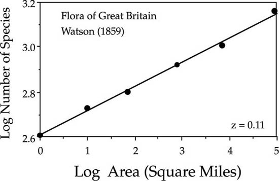
Before delving into the theory, it is useful to summarize briefly the major empirical patterns of species-area relationships and the current theories to explain them. For a thorough review of the subject, one should consult the book by Rosenzweig (1995). The empirical study of species-area relationships dates at least from H. C. Watson, who published the first known species-area curve for the vascular plants of Great Britain in 1859, the same year that The Origin of Species appeared (Williams 1964). Watson found a linear relationship between the logarithm of the number of species present and the logarithm of the area sampled, over areas ranging from a square mile to all of Great Britain (fig. 6.1). This is the most common pattern found on regional scales within relatively homogeneous landscapes (Gleason 1922, Williamson 1988, Rosenzweig 1995). The relationship is given by:
S = cAZ,
where S is the total number of species encountered in geographical area A, and c and z are fitted constants. This equation has come to be known as the Arrhenius species-area relationship after its most ardent champion (Arrhenius 1921), and is certainly now the most widely accepted relationship (Kilburn 1966, MacArthur and Wilson 1967, May 1975, Connor and McCoy 1979, Sugihara 1981). Note that if we let the constant c = ρz, where ρ is the mean density of individuals per unit area, then from our first principle we also obtain the number of species as a simple power function of the number of individuals J sampled S = Jz.
FIG. 6.1. Watson’s species-area curve for vascular plants of Great Britain, accumulating species from a starting point in Surrey. After Williams (1964) and Rosenzweig (1995).
Recently, Harte et al. (1999) have noted that the Arrhenius relationship is a power law that implies self-similarity in the distribution and abundance of species. Self-similarity implies that if one takes the ratio of any two areas, as long as one maintains a constant area ratio, the ratio of the number of species will also be invariant. Harte et al. assumed that the Arrhenius power-law relationship holds at all spatial scales, from which they could deduce the distribution of relative species abundance that is implied by a particular slope or z value. It is very interesting that the shape of the relative species abundance distribution implied by this power law is not a lognormal, but a distribution with a long tail of rare species that is highly reminiscent of a zero-sum multinomial distribution (chapter 5). However, there is a major problem with this assumption. The problem is that self-similarity in the species-area relationship is not maintained at all spatial scales, which destroys any potential functional relationship between a particular slope z and the distribution of relative species abundance. This implies that there are different scaling rules underlying the species-area relationship on different spatial scales. Therefore, the conclusion of Harte et al. that a one-to-one mapping exists between the exponent of the Arrhenius species-area power law and the relative species abundance distribution is not correct (Borda de Agua et al., manuscript). We shall now explore the causes for why the Arrhenius relationship does not hold at all spatial scales.
In a review of the patterns and causes of species-area relationships, Williamson (1988) posed four questions about these patterns. First, why is the Arrhenius relationship so common? Second, why do some surveys clearly not fit the Arrhenius relationship? Third, why is z the parameter of the Arrhenius relationship generally between 0.15 and 0.40? Fourth, why is there so much variation in z among surveys? I will address each of these questions from the perspective of the neutral theory, but out of Williamson’s original order.
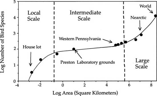
Williamson’s question number 2 has been empirically if not theoretically answered by Rosenzweig (1995). Rosenzweig found, in a review of a large number of species-area relationships, that the form of the species-area curve changes as a function of spatial scale. On local to global scales, species-area relationships are triphasic. The Arrhenius equation asserts that log-transforming both the number of species and area will linearize the species-area relationship, i.e., ln S = ln c+z·ln A. However, a linear log-log relationship is only typically obtained for intermediate spatial scales, but not on very local scales; and on large scales the slope increases. For example, Preston (1960) plotted the number of bird species over spatial scales ranging from an acre to the entire world, and obtained an S-shaped curve when log number of species was plotted against log area (fig. 6.2). In small contiguous areas, the curve was steep and curvilinear, then becoming shallower and log-log linear over intermediate to landscape and regional scales, and finally becoming steep once again over large intercontinental spatial scales, until the area of the entire world was included. The change in slope implies that scale-dependent changes in sampling units are occurring, a possibility of which Preston (1960) was clearly well aware. I will discuss this scale-dependent change in a more formal theoretical treatment shortly.
FIG. 6.2. Species-area curve for the world’s avifauna, spanning spatial scales from less than one acre to the entire surface of the Earth. The S-shaped curve suggests that the sampling units change as area is increased, from individuals, to species ranges, and finally to different biogeographic realms at local, regional to subcontinental, and finally to intercontinental spatial scales. Data from Preston (1960).
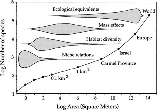
A similar S-shaped curve was obtained by Shmida and Wilson (1985), who plotted plant species-area relationships on local to global scales (fig. 6.3). They argued that the change in the form of the curve reflected changes in the biological determinants of plant species richness. On very local scales, niche-assembly rules would dominate. On somewhat larger spatial scales, mass effects and habitat diversity would become important. They define mass effects as an immigration subsidy from regional populations of a species that would go locally extinct without this immigration subsidy. Finally, they propose that at very large scales there are many “ecologically substitutable” species. As I will demonstrate in this chapter, however, a completely neutral dynamical theory of species-area relationships is fully capable of explaining such triphasic species-area curves without invoking any niche-assembly rules whatsoever.
FIG. 6.3. Shmida and Wilson’s (1985) hypothesis for the control of plant species diversity of different spatial scales, in relation to a species-area curve drawn from a local area in Israel (the mattoral region) to the entire world. Note the qualitatively similar shape to Preston’s (1960) curve for the world’s avifauna (fig. 6.2). Shmida and Wilson proposed that the biological determinants of species diversity changes from niche assembly on local scales, to habitat diversity and mass effects on intermediate scales, and to ecological equivalency on the largest spatial scales. The unified theory predicts these changes in the species-area relationship without positing any niche-assembly rules. Redrawn from Gaston (1994).
To classify these recurrent patterns, Rosenzweig (1995) offered a taxonomy of species-area curves in which he distinguished four types depending on the sampling scale and the evolutionary homogeneity or heterogeneity of the biota being sampled. Recasting his four types in the terminology of the unified theory, we have (1) species-area curves that arise in small areas within a single local community; (2) curves that arise in larger areas within a single metacommunity; (3) curves that arise among islands of an archipelago but still within the same regional metacommunity; and (4) curves that arise among different metacommunities with long-separate evolutionary histories. Rosenzweig’s classification can be simplified under the unified neutral theory. All four species-area patterns can be explained as different manifestations of the same underlying dynamical process, namely, zero-sum ecological drift operating on different spatial scales. However, in this chapter I limit the discussion to species-area relationships on continuous landscapes and do not consider type 3 further.
Taking a dynamical perspective, one realizes that the species-area relationship must represent a steady-state phenomenon just like the steady-state species richness on islands in the theory of island biogeography. In chapter 5 we proved that, in the implicit spatial case for “point mutation” specation, there exists a fundamental number θ which determines a unique relative species abundance distribution in the metacommunity at equilibrium between speciation and extinction. Now, simply allow the identical process of zero-sum ecological drift with speciation to occur over a continuous regional landscape. Then a steady-state spatially distributed “standing wave” of species diversity must also exist over this landscape. Every species originates at some point or in some region on the landscape, disperses out from this point or region of origin, and ultimately goes extinct. Therefore, our task is to find the steady-state spatial distribution of species richness and relative abundance predicted by the neutral theory. We assume here that this equilibrium arises in a metacommunity undergoing zero-sum ecological drift, random dispersal, and random speciation on a large but finite, homogeneous landscape.
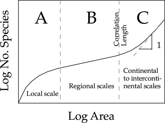
The theory’s explanation for the triphasic nature of species-area curves can be explained qualitatively as follows (fig. 6.4). At very local spatial scales, the species-area curve is very sensitive to the local commonness and rarity of species, as individuals are collected one by one. However, on regional to subcontinental spatial scales, the rate of encounter of new species depends much less on relative species abundance, and more on rates of speciation, dispersal, and extinction, and the resulting steady-state geographic ranges of species. At very large, intercontinental scales, species accumulate faster again as major barriers to dispersal are crossed—barriers between different biogeographic realms with long separate evolutionary histories (Rosenzweig 1995). There is an inflection in the species-area curve separating regional and very large scale sample areas, where the curve bends upward. This inflection point is the correlation length of the biogeographic process. The correlation length is very important because it specifies the natural length scale of the dynamical speciation-dispersal-extinction process, which in turn defines how big the natural biogeographic evolutionary units are on the metacommunity landscape. I will have more to say about biogeographic correlation lengths later.
FIG. 6.4. The qualitative shape of the triphasic species-area curve, as predicted by the unified neutral theory. On local spatial scales (region A) the species accumulation curve is most sensitive to relative abundance of species in the local community. On regional spatial scales (region B), the species accumulation curve is less sensitive to relative species abundance and more to the encounter of the ranges of species at steady state between speciation, dispersal, and extinction. On very large spatial scales (region C), the correlation length of the biogeographic process has been exceeded, and sampling is of biogeographic realms with completely separate evolutionary histories. The correlation length defines the natural length scale of the biogeographic process.
According to the unified theory, the answer to Williamson’s question number 4 is that slopes of species-area relationships vary so much because they depend dynamically on rates of speciation, dispersal, and extinction over regional to continental to intercontinental landscapes.
In general, sampling across dispersal barriers is always expected to steepen species-area curves because species that have not managed to cross the barriers will be relatively abruptly encountered for the first time. MacArthur and Wilson (1967) themselves invoked a verbal dynamical model to explain why species-area curves on the continuous mainland tend to exhibit shallower slopes than species-area curves for island archipelagos. This difference was attributed in part to the greater difficulty of dispersing to and among islands relative to dispersing among contiguous mainland communities, and in part to higher extinction rates on islands (MacArthur and Wilson 1967, Brown and Gibson 1983, Rosenzweig 1995). As we will show below, the unified theory predicts that the slope of the species-area curve will approach unity because at very large sampling scales, regional biogeographic processes become independent and uncorrelated.
I now turn to a more formal development of the neutral theory of species-area relationships. I first consider the theoretical species-area and species-individual curves for the metacommunity under the assumption of no dispersal limitation. Then I introduce dispersal limitation and determine how it affects the expected curves. Two of Williamson’s questions still remain, namely: Why is the Arrhenius relationship so common (question 1). And, Why do the slopes (z values) of these relationships commonly lie between 0.15 and 0.4 (question 3)? I will offer the unified theory’s explanations for these patterns in due course.
A dynamical theory of species-area relationships on all spatial scales is most easily approached through the theory for the metacommunity. We can relate the sample of size J to area by means of our first principle (chapter 3), which states that landscapes are essentially always biotically saturated with individuals of a specified community or taxon. Thus, J = ρA, where A is the area occupied by J individuals and ρ is mean density. As noted in chapter 5, this relationship also holds for the full metacommunity, JM = ρAM, so that we can express the fundamental biodiversity number θ as a simple linear function of area and density of organisms:
θ = 2ρAMν.
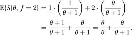
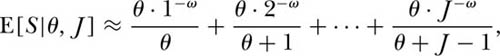
This relationship implies that a function of θ exists which specifies both the species-individual and the species-area relationships. If dispersal is not limited, then the unified theory makes a simple prediction for the cumulative species-individual and species-area curves. We can easily derive the expected number of species S in a sample of J individuals chosen randomly from the metacommunity from the formula for the probability, Pr{S, n1, n2, . . . , nS} (see chapter 5). Thus, for J = 1, the expected number of species is clearly unity (from the formula, θ/θ). For J = 2, the probability of obtaining a single species with two individuals is 1/(θ + 1), and the probability of two species each having a single individual is θ/(θ + 1). Thus the expected number of species in a sample of two individuals is the sum of the two expectations: E{S|θ J = 2} = E{S = 1|θ J, = 2} + E{S = 2|θ, J = 2}, or
Continuing in this manner, one can show by induction that for arbitrary J,
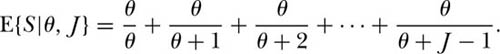
This expectation is for the species-individual curve sampled at random from the equilibrium metacommunity obeying zero-sum ecological drift. It specifies the expected rate of addition of species as individuals are collected one by one, and in principle can be extended out to the metacommunity size, JM. Note that we can convert this expectation into a species-area curve, E{S|θ, ρ, A} = Σθ/(θ+ρA−1) simply by making the variable substitution J = ρA. This expectation was originally derived by Ewens (1972) for the sampling of neutral alleles in the “infinite allele” case, which is identical to the ecological drift case. If one applies this to sampling in a spatial context, however, it only applies under the limiting assumption of complete mixing of the species, i.e., no dispersal limitation, as we shall discuss in a moment.
We can now show, from the equation for the metacommunity species-individual curve, that the fundamental biodiversity number θ, which derives from the theory of zero-sum ecological drift, provides a justification for Fisher’s α, the diversity parameter of the logseries distribution (Fisher et al. 1943). Recall from chapter 2 that Fisher’s formula for species accumulation is
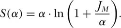
As JM increases, S(α) becomes asymptotic to α · ln(JM/α), a straight line on a graph of S vs. ln(JM/α) with slope α.
The theoretical species-individual curve predicted by θ and zero-sum ecological drift can be approximated closely by
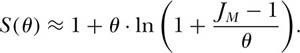
Note that as JM increases, S(θ) also becomes asymptotically parallel (displaced by unity) to ln(JM/θ) with slope θ. Thus, we have a very important result, namely that, as metacommunity size JM, increases toward infinity. Fisher’s α is asymptotically identical to the fundamental biodiversity number θ:
and the metacommunity distribution becomes asymptotically identical to Fisher’s logseries. This result was also discovered for Ewens’s formula in the infinite neutral allele case in population genetics (Watterson 1974). Because θ is not precisely equal to α, the distribution of relative species abundance in the metacommunity will be very similar to, but not precisely identical to, the logseries.
The implications of this simply stated result are quite profound. We have now connected Fisher’s logseries distribution to the theory of metacommunities undergoing pure ecological drift. We therefore conclude that if relative species abundances are well described by the logseries and Fisher’s α, then these data are consistent with zero-sum ecological drift and with random sampling of the metacommunity.
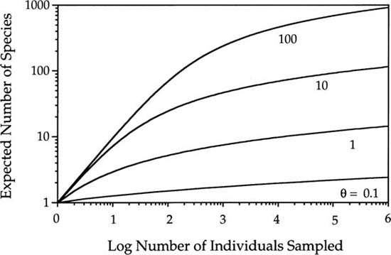
In the limiting case of no dispersal limitation, the meta-community equation E{S|θ, J} gives the expected species-individual and species-area curves at all spatial scales, from local to global. It works on local scales when J is small, and on regional scales when J is large. Figure 6.5 illustrates the expected metacommunity species-individual curves for three orders of magnitude of variation in θ on a double-log transformed plot. (Recall from above that we can convert cumulative individuals into cumulative area.) Note the curvilinearity of the lines on local scales, demonstrating the failure of the Arrhenius relationship, S = cAz, on local scales (Williamson’s question number 2). As mentioned above, this is because the species-area sampling process is especially sensitive to relative species abundance when J is small. At first, species are added fast with increasing sample size because the common species are collected quickly in the first samples, making the species accumulation curve rise steeply. Later, the curve rises more slowly as successively rarer and rarer species are collected. The theoretical curves never reach an asymptote, however. This is so because the infinite series  diverges as J → ∞. Divergence is perfectly acceptable because an infinite number of species can be accommodated among an infinite number of individuals. Of course, real metacommunities are not infinitely large, although JM is a very large number, and so, there can only be a finite number of possible species. Once a value of θ has been estimated, the expected number of species in a sample of any size can be determined, including, in principle, the entire metacommunity, assuming JM can be reasonably estimated. Note also that because
  , successively rarer species are added at an ever decreasing rate as the number of individuals increases.
FIG. 6.5. Expected species-individual curves for values of the fundamental biodiversity number θ ranging over 3 orders of magnitude from 0.1 to 100. Note double log scales. These are expectations for a random sample of individuals from the metacommunity (no dispersal limitation). Individuals sampled can be converted to area by making the variable substitution, J = ρA.
The curves in figure 6.5 also reveal the strong sensitivity of the species-individual and species-area curves to the fundamental biodiversity number θ. In a sample of a thousand individuals, for example, a community with a θ value of 100 will exhibit about twenty times as many species as a community with a θ value of unity, two orders of magnitude smaller. Because of the nonlinearity of the species-individual curves, however, two communities differing in their θ’s do not maintain a constant ratio of species diversity as sample size varies. Note that as J becomes larger, the species-individual curves become more similar in slope and approach linearity on the double-log plot (fig. 6.5). This anticipates the log-log linear species-area relationships that the theory predicts on intermediate (regional) spatial scales.
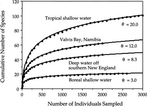
The similarity of the theoretical curves in figure 6.5 to many empirically derived species-individual curves is readily apparent. Nearly all such curves are initially steep and then become shallower, whether the curves are plotted arithmetically or logarithmically. For example, figure 6.6 shows a sample of the species-accumulation curves reported by Sanders (1969) for benthic marine communities collected in transect trawls at four sites spanning a large latitudinal range. These curves were constructed from a series of small, scattered trawls and, therefore, as noted above, are expected to be closer to a random sample of the metacommunity. In fact, May (1975) found that these curves were well fit by Fisher’s logseries, meaning that they are also expected to be fit by the unified theory’s metacommunity distribution.
FIG. 6.6. Species-individual curves for benthic invertebrate conmmunities at four sites spanning a broad latitudinal range. Dots are Sanders’s observations; solid lines are the expected curves. Redrawn from May (1975).
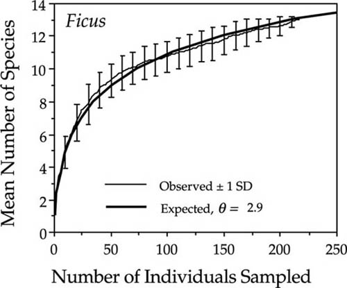
The theoretical metacommunity species-individual curve assumes random sampling, but it nevertheless also occasionally fits the data for local community species-individual curves quite precisely. A case in point is the excellent fit obtained for the species-rich genus of figs, Ficus (Moraceae), in the 50 ha plot on Barro Colorado Island, which yielded a fitted θ of 2.9 (fig. 6.7). The observed curve represents the mean of 10 randomized drawings of all individuals of the 13 fig species in the plot. The error bars are ± 1 standard deviation of species number for a given number of individuals drawn.
FIG. 6.7. Species-individual curve for 13 species of the genus Ficus in the 50 ha plot on Barro Colorado Island. The expected curve is a maximum likelihood estimated θ of 2.9. The error bars are ±1 standard deviation of 10 random sampling of Ficus trees in the plot. The meta-community distribution fits this genus well, probably because figs are very good dispersers.
When the metacommunity species-individual curve fits local data this well, it either means that the community or taxon is composed of species that are very good dispersers and are well mixed over fairly large landscape scales, or else that the sampling regime compensates to some degree for dispersal limitation. Ficus is a genus of stranglers or free-standing trees that are pollinated over relatively long distances by small windborne agionid wasps, and whose seeds are widely dispersed by fruit bats, frugivorous birds, and monkeys. This view of fig population structure is supported by studies of fig population genetics that indicate little genetic differentiation over large distances (Nason et al. 1996).
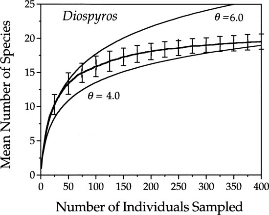
More generally, however, because of dispersal limitation, the metacommunity species-individual curve is not expected to fit local communities well, according to the unified theory. Consider, for example, the species-individual curve for the genus Diospyros (Ebenaceae), a species-rich genus of understory trees in the 50 ha plot at Pasoh Forest Reserve in Malaysia (fig. 6.8). These typically small-stature trees produce large multiseeded berries that are dispersed locally by ground mammals. After an initially rapid rise, the observed curve for Diospyros continues rising but more slowly than the theoretical curves, two of which are shown for comparison.
FIG. 6.8. Species-individual curve for 25 species of the genus Diospyros in the 50 ha plot in Pasoh Forest Reserve, Malaysia. Two theoretical curves for θ = 4 and θ = 6 are compared with the observed curve. The error bars are ±1 standard deviation of 10 random samplings of Diospyros trees in the plot. The metacommunity distribution does not fit this genus because its species are poor dispersers. Increasing dispersal limitation on larger spatial scales causes the increasing lag in observed species accumulation as sample size increases, relative to the metacommunity curves that assume unlimited dispersal.
The local species-individual curve will rise more slowly under dispersal limitation than without it. Unfortunately, no analytical result of the effect of dispersal limitation on the species-individual curve is currently available. However, we can derive an approximation that appears to be quantitatively very close to the true function. In continuous space, note that the probability m of a local death being replaced by an immigrant must be a monotonically decreasing function of the number of individuals, J, occupying the given area, A. The probability of immigration is unity for J = 1 (chapter 4), and m → 0 as J → ∞. As noted previously, the species-individual curve approaches the power law S = Jz, which implies that the probability of immigration must decline due to dilution from increasing J in proportion to the inverse of J raised to some power, i.e.,
m(J) ≈ J−ω,
where the dispersal limitation parameter ω ≥ 0. Incorporating this function into the equation for the local species-individual curve, we obtain the following function for the rate of addition of species under dispersal limitation:
or that 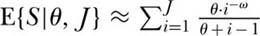 . Note that when ω = 0, this equation reduces to the limiting metacommunity case of no dispersal limitation. It should be stressed that this equation is appropriate only for dispersal limitation on local spatial scales. On regional to continental spatial scales, the effect of dispersal limitation is actually to increase the slope of the species-area curve (see below).
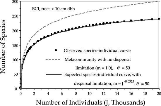
I illustrate the goodness of fit of the species-individual function under dispersal limitation to the observed species-individual curve data for trees > 10 cm dbh in the 50 ha plot on Barro Colorado Island (fig. 6.9). In chapter 5 we found that the dominance-diversity curve for BCI was well fit with a θ of 50 and a probability of immigration m of 0.10. The species-individual curve for BCI gives us a more precise method for measuring the probability of immigration, because it describes how species number increases at the level of the addition of individuals rather than of whole species. Moreover, we can now estimate the average community-level rate at which the probability of immigration declines as we increase the sample size, J, by estimating parameter ω. Figure 6.9 shows that the metacommunity species-individual curve considerably exceeds the observed number of species for a given number of individuals. It overestimates the true number of species in the 50 ha plot by more than a quarter (28% higher). However, if we take dispersal limitation into account (m < 1) and estimate the rate at which mean dispersal limitation increases with J, then we obtain a very good fit to the observed species-individual curve, with a maximum likelihood estimate for ω of 0.0325 for a θ once again of 50. Similar curves are obtained for the 50 ha plot in the Pasoh Forest Reserve. A more detailed discussion of species-area and species-individual curves in these plots can be found in Condit et al. (1996).
FIG. 6.9. Species-individual curve for trees > 10cm dbh in the 50 ha plot on Barro Colorado Island, Panama. The observed curve (dots) was obtained by averaging species richness in randomly chosen contiguous areas containing a given number of individual trees. The metacommunity species-individual curve overestimates the number of species in the plot by 65 species (28%). The parameters of the species-individual curve under dispersal limitation were estimated by maximum likili-hood, and yielded θ = 50 and ω = 0.0325.
I now turn to regional and larger spatial scales, the domain in which Rosenzweig’s (1995) species-area curve types (2) and (4) are found. As we move from local to regional to global spatial scales, dispersal limitation becomes far more important than relative abundance in controlling the species-area relationship. Thus the proportion of dispersal-limited species increases as area increases. Decreasing the average dispersal rate increases the proportion of species that will be dispersal limited for an area of a given size.
The neutral theory predicts opposite effects of dispersal limitation on the species-area curve on local versus regional scales. On local scales, dispersal limitation reduces the slope of the species-area curve because rare species are not encountered as fast as would be expected under random spatial mixing of species. On regional scales, dispersal limitation increases the slope of the species-area curve. This is not predicted by the theoretical metacommunity species-area curve, which exhibits an ever shallower slope with increasing area. However, this curve was derived assuming random sampling without dispersal limitation. The effect of dispersal limitation becomes increasingly pronounced as the sampling scale exceeds the steady-state range sizes of more and more species (i.e., exceeds the correlation length L), which in turn increases the encounter rate of previously untallied, dispersal-limited species. Therefore, the unified theory’s explanation for the change in the form of the species-area curve on different spatial scales is that the effect of dispersal limitation on the species accumulation rate changes from negative to positive with increasing spatial scale.
We can explore this change in the form of the species-area relationship more fully using two spatially explicit models of metacommunity drift on intermediate and large spatial scales. I first discuss the model of Durrett and Levin (1996), who studied a version of the “voter model” (Holley and Liggett 1975, Silvertown et al. 1992) applied to the species-area problem. The name “voter model” was originally inspired by theoretical studies of simple models of the spread of opinions. Imagine “voters” standing on an infinite gridded plain, with one person in each grid location. Each person keeps his or her opinion for an exponentially distributed time period, after which he or she adopts the opinion of a neighboring individual, such that the person located at (x) picks the opinion of the person at location (y) with probability p(x, y). Durrett and Levin (1996) added mutation or “speciation” to this model, whose spatial dynamics evolves according to the following rules. Let the “species” occupying a given site be identified by some random number chosen on the interval (0, 1). Rule 1 is that sites are always occupied by some species, but at rate δ, an individual dies and is replaced by an individual of a species chosen at random from the neighborhood, with probability p(|y − x|). Rule 2 is that at rate ν, ν,  δ, the occupant of a site changes or “speciates” into a new type
  (0, 1) not seen before.
Durrett and Levin (1996) cite proofs in Bramson et al. (1996) of the following results for the special case of p(|y − x|) = 1/4 when |y − x| = 1, or that immigration is possible in one time step only from the 4 immediate neighbors (ignoring neighbors on the diagonals). They report approximations that become more exact as the speciation rate ν → 0. They relate their results to the correlation length L of the biogeographic process. In their model this distance is defined as the inverse of the square root of the speciation rate: 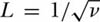 . This number is approximately equal to the expected distance under a two-dimensional random walk that an average species moves over its metacommunity lifetime from the site of its origination. They were able to prove several useful results, three of which will be mentioned here. First, they showed that the slope of the log-log species area curve approaches zero as the speciation rate ν → 0, and that when ν is small, this slope is approximately
where S is the number of species. Note that 2log L is simply the logarithm of a square area whose side is equal to the correlation length L. Second, they showed that at length scales less than L, as ν → 0 the number of species at equilibrium approaches a constant. This is a weaker theorem than in the present theory of ecological drift, where one can prove that when ν = 0, there can only be a single surviving species at equilibrium (chapter 4); but it agrees with the theory.
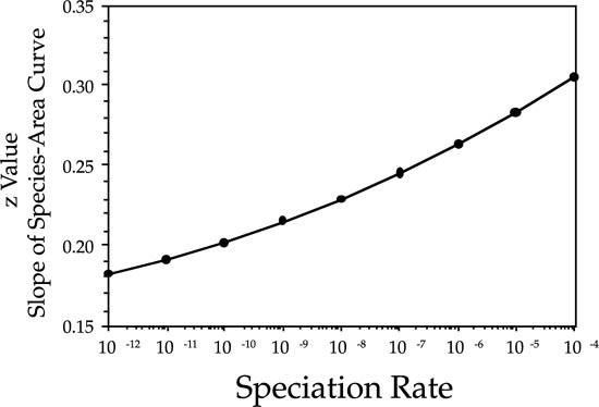
Durrett and Levin (1996) used their approximation for the slope of the log-log species area curve to provide a partial answer to Williamson’s (1988) last question, which was: Why is there so much variation in the slope of species-area curves? If we insert various values of the speciation rate, substituting 1/ for L, we obtain the relationship between speciation rate and z value shown in figure 6.10 for length scales less than L. The z value is low for slow rates of speciation and becomes progressively steeper for faster rates. Note also that the relationship is curvilinear: z values increase ever faster as the speciation rate increases.
Durrett and Levin (1996) showed that on length scales that are much larger than the correlation length L, the slope of the species-area curve becomes steeper and approaches unity. The slope increases to near unity because events become uncorrelated on length scales >> L—spatial scales that are large relative to the equilibrium range sizes and dispersal distances taken by species during their evolutionary lifetimes in the metacommunity. This explains the phenomenon of the steepening species-area curves discovered by Preston (1960) and Shmida and Wilson (1985) at large spatial scales (figs. 6.2 and 6.3). Rosenzweig’s (1995) puzzlement over the fact that “the [species-area] curve among provinces has z values near unity” (p. 379) is also now explained. This effect is another reflection of the fact that there is extreme dispersal limitation between major biogeographic provinces.
FIG. 6.10. Relationship between the z value (slope of the Arrhenius species-area curve) and the speciation rate, according to an approximation derived by Durrett and Levin (1996) for small ν.
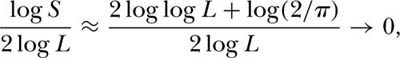
Another useful result of Durrett and Levin’s (1996) model is that it provides a theoretical justification for the prevalence of the log-log species-area relationship of Arrhenius (1921) on intermediate spatial scales—as does the present theory. This addresses Williamson’s (1988) question number 1. Durrett and Levin’s formula for the slope of the species-area curve is closely related to the unified theory’s equation, S = 1+θ·log[1+(J −1)/θ]. To see this, observe that Durrett and Levin studied, in unified theory terms, a finite meta-community of size L2 (since there was one individual per grid location), in which JM = ρA = L2. For large metacommunities, JM >> θ, and, taking logs, log S ≈ log[log(JM) − log θ] + log θ ≈ log log(JM) + log θ = log(2 log L) + log θ = log log L + log 2 + log θ. Dividing both sides of the equation by 2log(L) to compute the slope of the species-area curve, we obtain
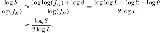
This formula clearly shows the influence of both JM and θ on the slope of the approximately log-log species-area curve for large JM or L. It differs somewhat from the formula of Durrett and Levin, which is expected since their formula was derived for a specific case of dispersal limitation (the voter model with p(|y − x|) = 1/4 when |y − x| = 1), whereas the unified neutral theory’s formula is based on the metacommunity species-individual curve with no dispersal limitation. Using the above equation, we can also calculate how the slope of the metacommunity species-individual curve changes with the number of individuals sampled. The slope of the tangent at any J is approximately [log log L + log θ] log J for J > 1. From this expression, one could also construct the approximate species-individual curve for the metacommunity.
In contrast, the species-area slope calculation of Durrett and Levin cannot be used to compute the species-area curve for a given speciation rate. This is because in their formulation one cannot vary the area parameter—the square of the correlation length L—without simultaneously varying the speciation rate ν. A second “problem,” more apparent than real, would seem to exist with the speciation rates that Durrett and Levin (1996) needed to obtain z values similar to those of observed species-area curves (fig. 6.10). These speciation rates ranged from 10−4 to 10−12 per birth, which might seem to be unrealistically high.
These “problems” disappear entirely in the unified theory with the introduction of the fundamental biodiversity number θ, which applies equally well to the voter model with speciation studied by Durrett and Levin. Because θ is a product of JM and ν, one can separate the effects of metacommunity size and speciation rate for the first time. A large meta-community with a low speciation rate can have an identical species-area curve as a small metacommunity with a high speciation rate, so long as the fundamental biodiversity number θ remains the same (under point mutation speciation). Increasing the metacommunity size while holding the speciation rate constant will increase the slope of the equilibrium species-area curve, just as increasing the speciation rate will. Increasing JM increases the number of speciation events per unit time because absolutely more births occur per unit time in a large metacommunity than in a small one.
I now study a somewhat more complicated model by simulation, one that is similar to the voter model, except that now we allow each grid location to be a local community of arbitrary size J > 1. Let each local community be coupled in a single time step through dispersal with probability m per birth with the local communities that comprise its immediate neighbors. The equations for the local dynamics of the ith species can be written down as follows. Let (x, y) be the coordinates and index name of the local community. Let deaths in local community (x, y) be replaced by local births or by immigrants with probability m in one time step from the surrounding frame of 8 neighboring communities, located at (x − 1, y − 1) to (x + 1, y + 1). This neighborhood is known as the “Moore neighborhood” in cellular automata theory. The metacommunity abundance parameter Pi is thereby replaced by the current abundance of species i summed over the surrounding frame of neighboring communities.
Including the probability of speciation, ν, the transition probabilities for the ith species having abundance Ni(x, y) in the local community (x, y) with immigration from the immediate neighboring communities in one time step, then become
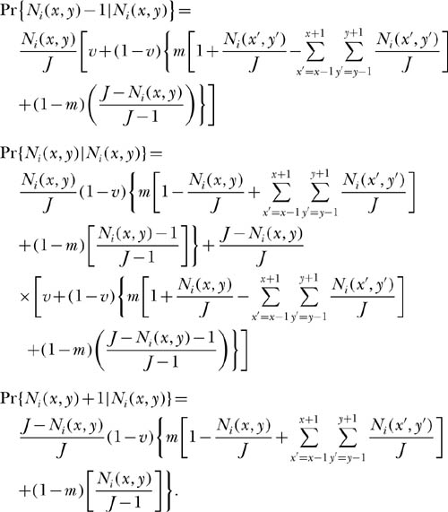
For example, the first equation is the probability that species i in local community (x, y) will decrease by one individual in the next time step. For this to happen, an individual of the ith species in community (x, y) must die and not be replaced by another individual of species i. This replacement individual can be a new species (with probability ν) or be a preexisting species (with probability 1 − ν), in which case it can either be an immigrant or a local birth of some species other than i. Note that Pi is no longer a constant, as it was treated in chapter 4, but is replaced by the current relative abundance of the ith species in the frame of local communities surrounding the focal community (x, y). Also note that m is no longer the probability of immigration from the entire metacommunity, but only from the surrounding local communities.
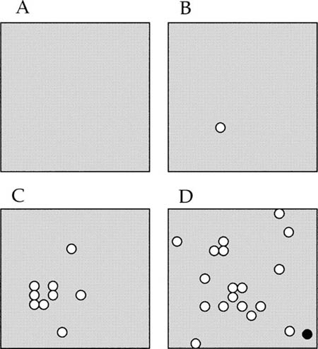
Suppose the initial ancestral condition is a single, monodominant species whose individuals saturate the metacommunity plain and all local communities. Now start an engine of speciation, such that a new species arises somewhere on the plain with probability ν per birth. New species will arise at random points of origination on the finite but large landscape and, if they are lucky, will multiply and disperse before ultimately going extinct. Figure 6.11 is a cartoon illustrating the spatially explicit process of zero-sum ecological drift in the metacommunity. The figure shows four early stages in the evolution of a steady-state species diversity and its geographical dispersion over a small piece of the infinite plain. Initially, at t = 0 (panel A), the plain is occupied everywhere by a single, monodominant species (shading). At some later time, t = t1 (panel B), a new species originates (white circle) from the original species. By time t = t2 (panel C), the second species has increased in abundance and spread out from its point of origin. At any given moment each species will have a distribution that reflects its unique history of repeated colonizations and extinctions in local communities up to that point. Later, by time t = t3 in this cartoon (panel D), a third species has arisen (black circle).
FIG. 6.11. Early stages in the evolution of species diversity on a portion of a homogeneous plain harboring a metacommunity. Initially (A), one species is monodominant in the metacommunity (shading). Later (B), a second species (white circles) originates, and subsequently (C) spreads out from its point of origination. Still later (D), a third species arises (black circle). The process continues indefinitely, and eventually a stochastic metacommunity steady-state species diversity between speciation and extinction is achieved.
Let us now study numerically the dynamical behavior of a metacommunity gridded into identical local communities, each of whose species obeys the above equations of zero-sum ecological drift. Conceptually, the metacommunity can be infinite in size, but in practice only finite representations are possible on a computer (and in the real world). One has basically two choices in modeling finite metacommunities: either with or without edges. There are advantages and disadvantages to both representations. To implement a metacommunity model without edges, one “wraps” opposite sides of the grid into a torus so that they become adjacent. The advantage of the torus model is that it completely eliminates edge communities and edge dynamics. However, it is unclear that species-area relationships will be the same on a torus and on a plain, particularly if the torus is relatively small. Moreover, to my knowledge there are no toroidal communities in nature, and their behavior is difficult to show in planar representations. One must disconnect the edges and “unwrap” the torus; but in so doing, the resulting maps make it appear that populations can suddenly jump from one side of the metacommunity to the other. This could introduce a significant artifact into the analysis of species-area relationships under dispersal limitation.
Of course, the disadvantage of planar models with edges is edge-effect dynamics. Local communities along edges behave differently because they have smaller source areas and more restricted immigration than local communities far from edges. The result is that edge communities are effectively more isolated and subject to ecological drift. They will generally exhibit steeper dominance-diversity curves than centrally located communities. Nevertheless, I prefer the planar approach, but one in which species-area relationships are studied far from edges to reduce edge-effect dynamics as much as possible. I simulated a relatively large metacommunity (101 × 101 local communities), but restricted my analysis of regional species-area relationships to a grid of 21 × 21 local communities at the center of the metacommunity, which comprises only 4.3% of the total metacommunity area. In the simulations that follow, I chose a local community size of J = 16 individuals unless otherwise indicated.
The first important result to establish is that a nontrivial metacommunity equilibrium species richness and relative species abundance distribution exists in the spatially explicit theory. We need to know that this equilibrium is unique and independent of initial conditions, and that it is similar to the equilibrium predicted by the metacommunity theory in chapter 5, when we treated space implicitly. These equilibria will not be identical, however, because dispersal limitation is present in the spatially explicit theory, whereas it is absent in the spatially implicit metacommunity theory. I am unable to prove uniqueness analytically in the spatially explicit model for local community size J > 1. However, simulation results leave no doubt that the equilibrium is nontrivial and unique, as is demanded by the spatially implicit theory given in chapter 5.
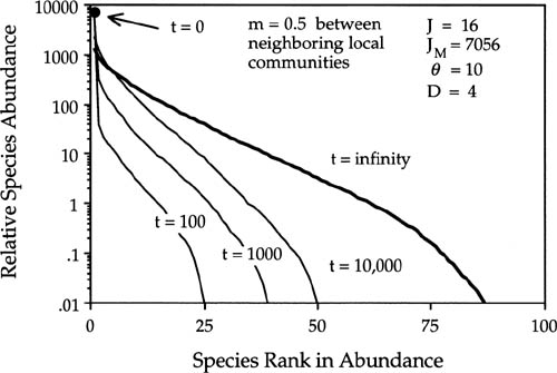
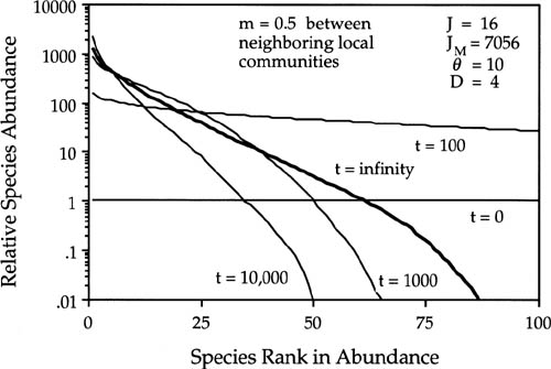
Figure 6.12 shows the convergence on the equilibrium metacommunity dominance-diversity curve starting from initial monodominance, for a case in which D = 4(25% mortality per disturbance cycle), m = 0.5, and θ = 10. Figure 6.13 shows convergence to the same equilibrium from initial conditions of “infinite” diversity at the other extreme, with one individual of each species at the outset. The curves represent means of one hundred simulations. In figure 6.13 the horizontal line at unity for t = 0 is the initial conditions of infinite diversity. The approach to equilibrium is more complex in this case than under monodominance (compare figs. 6.12 and 6.13). In the case of “infinite” initial diversity, it would appear from figure 6.13 that all species become more abundant early on, but in fact only some species do so. Figures 6.12 and 6.13 truncate the relative abundance distributions at the one hundred most common species.
FIG. 6.12. Transient approach from initial conditions of monodominance to the equilibrium metacommunity dominance-diversity under dispersal limitation. Local community size J = 16. Metacommunity size JM = 7056 individuals; m = 0.5; θ = 10. The bold line is the equilibrium dominance-diversity curve (t = 10,000 birth-death cycles). The curves are shown only for the one hundred most common species. A stochastic equilibrium is achieved that is indistinguishable from that obtained under initial conditions of infinite diversity (cf. fig. 6.13).
FIG. 6.13. Transient approach from initial conditions of “infinite” diversity to the equilibrium metacommunity dominance-diversity under dispersal limitation. Local community size J = 16. Metacommunity size JM = 7056 individuals; m = 0.5; θ = 10. The bold line is the equilibrium dominance-diversity curve (t = 10,000 birth-death cycles). The curves are shown only for the one hundred most common species. A stochastic equilibrium is eventually achieved that is indistinguishable from that obtained under initial conditions of monodominance (cf. fig. 6.12).
Although I have illustrated only one numerical case in these two figures, the following conclusions are general and hold for any and all values of the theory’s parameters in the spatially explicit unified theory. First, the equilibrium distribution of metacommunity diversity is independent of initial diversity conditions, as was the case in the spatially implicit theory. Second, the expected diversity distribution is uniquely determined by just three parameters: the fundamental biodiversity number θ, local community size J, and the probability of migration m. Finally, the approach to diversity equilibrium is much faster from initial conditions of infinite diversity (every individual is of a different species) than from initial conditions of monodominance.
This asymmetry stems from two factors. First, metacommunity species that are abundant and widespread are extremely resistant to displacement and extinction. Second, completely new metacommunity diversity must await speciation events, which are very infrequent, and even then the probability of successful establishment of new species is likely to be very low. This is particularly true under the “point mutation” model of speciation. However, if new species arise by “random fission,” then successful establishment of new species is more likely. These results have important implications for conservation. When most species are rare, metacommunity diversity will be easy to lose, whereas once metacommunity diversity is lost, it will be much harder and slower to recover.
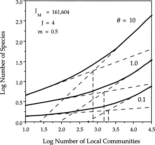
Having now established that a unique equilibrium dominance-diversity curve arises in the metacommunity in the spatially explicit unified theory, I return to the subject of species-area relationships. We are interested in the predictions of the spatially explicit model for species-area relationships on intermediate (regional) spatial scales—the scales on which the log-log linear Arrhenius (1921) relationship holds—and then on still larger spatial scales. Specifically, we wish to determine how variation in the fundamental biodiversity number θ and the dispersal rate m affect both the unit area intercepts (α diversity) and the slopes (z values, β diversity) of the equilibrium species-area curve at these spatial scales.
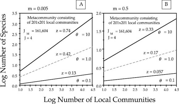
I examined steady-state species-area relationships on an intermediate spatial scale for a minimum area spanned by nine local communities to a maximum area representing 121 local communities each of size J = 4 sampled from the center of a metacommunity of 201 × 201 local communities, far from any edge. The initial conditions of the metacommunity were set to the dominance-diversity distribution dictated by a given θ for a metacommunity of size JM = 201 × 201 × 4 individuals under no dispersal limitation. Species were assigned initial locations at random. I first established that 20,000 birth-death cycles with one death per cycle in each local community (5000 complete turnovers of the metacommunity) was more than adequate time for the species-area curves to equilibrate. Several typical sets of results are shown in figure 6.14. Each species-area curve in the figure represents a mean of one hundred simulations for a given θ and m. In the left panel, m = 0.005, a low rate of immigration, and in the right panel the probability of immigration is one hundred times greater (m = 0.5).
FIG. 6.14. Effect of varying the fundamental biodiversity number θ and the probability per birth of immigration m, into a local community from neighboring communities on the small-area intercept (α diversity) and the slope (z value, β diversity) of the species-area curve at regional spatial scales. Metacommunity consists of 201×201 local communities, each of size J = 4. (A) Immigration rate m = 0.005. (B) Immigration rate m = 0.5.
Several general conclusions are illustrated by these graphs that are consistent with the analytical results of chapter 4. First, the theory shows that log-log linear Arrhenius power law species-area curves are always obtained on intermediate spatial scales. Second, the intercept and the slope (z value) of the species-area curve are controlled by two parameters: the fundamental biodiversity number θ and the probability of immigration m. The effects of the two parameters differ. Increasing θ increases the z slope as well as the small-area intercept, raising both α and β diversity. Conversely, increasing the dispersal rate m decreases the slope of the species-area curve (lowering β diversity) but increases the small-area intercept (raising α diversity). The reasons for these contrasting effects are simple. When dispersal rates are rapid relative to speciation rates, z values are low and species-area curves are shallow. But when dispersal is very limited, then many new and local species will be encountered as sample area increases, and the species-area curve will have a steeper slope. Quantitatively, in this example (fig. 6.14) a 100-fold increase θ from 0.1 to 10 resulted in about a 5.7-fold increase in the z value, whereas a 100-fold increase in m from 0.005 to 0.5 resulted in a 55%–60% decrease in the z value. More generally, the ratio of increase or decrease will vary depending on the range of actual values of θ and m.
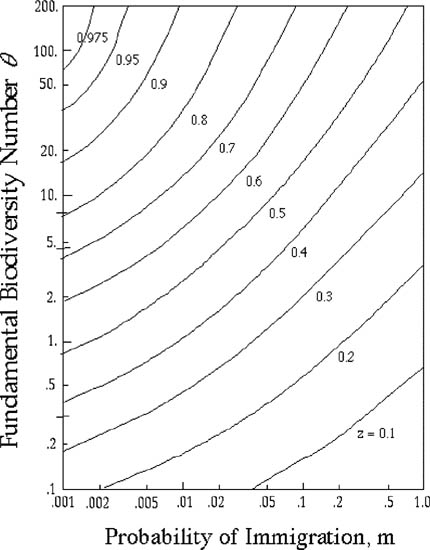
A large number of simulations show conclusively that the unified theory always generates log-log linear Arrhenius type species-area curves on intermediate spatial scales. Therefore, the more general question of how θ and m affect the z value of the species-area curve can now be answered. Figure 6.15 plots contours of equal slope z as a function of θ and m. In the figure, I have varied θ over slightly more than three orders of magnitude, from 0.1 to 200, spanning much of the range of θ’s observed in nature (with the possible exception of some highly diverse microbial communities; see chapter 5). I have also varied immigration rate m over three orders of magnitude, from 0.001 to 1.0. The precise location of the contours of iso-z lines in θ − m space depends upon the exact nature of the dispersal function used in the model, but several qualitative conclusions are universally true.
FIG. 6.15. The effect of varying the fundamental biodiversity number θ and the probability of immigration m on the slope (z)-value of the Arrhenius species area curve at regional spatial scales, according to the unified theory. Note that z → 1 as θ → ∞ and that z becomes smaller as m → 1. It should also be noted that m = 1 in the spatially explicit model does not correspond to infinite dispersal, as in the implicit-space theory, but rather to a case in which all local-community deaths are replaced by immigrants from the Moore neighborhood of immediately adjacent local communities. Results are from simulations (see text).
First, a general result is that predicted z values are steep for large θ and small m, and shallow for small θ and large m. Second, the effect of an incremental change in the immigration or dispersal rate on the slope of the species-area curve is larger for large m than for small m. Note that as m decreases, the isoclines of equal z become shallower and more nearly parallel to the m-axis. Generally, for very low values of m (e.g., 10−5 or lower), changes in m have very little effect on the species-area slope and the dominant variable affecting z values is simply the fundamental biodiversity number θ. For a given θ, it requires a lower immigration rate to achieve a given z value when θ is larger than when θ is small. From this we conclude that the slope of the species-area relationship becomes less sensitive to (more independent of) the dispersal rate, and relatively more dependent on the fundamental biodiversity number, as the connectivity or “panmixis” of the metacommunity decreases.
Finally, figure 6.15 also gives an answer to the last remaining question of Williamson (number 3), namely, why do so many slopes of species-area relationships fall between 0.15 and 0.40? The unified theory’s explanation is simply that a broad region of θ − m parameter space exists for which z values lie between 0.15 and 0.4. Note that we are referring here to species-area relationships within continuous biogeographic landscapes (Rosenzweig’s type 2 curves), not to the species-area curves obtained over an archipelago of discrete islands or habitat patches of different sizes (Rosenzweig’s type 3 curves).
I now consider very large spatial scales, larger than the correlation length L, i.e., the spatial scale on which the species-area curves begin to steepen. At these large spatial scales, biogeographic processes become less and less correlated as the spatial sampling scale exceeds the distance separating dynamically independent biogeographic regions (Rosenzweig’s type 4 curves).
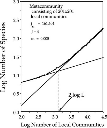
It is possible to define a measure of the correlation length that is more informative of the actual spatial scale on which the inflection point in the species-area curve occurs than the metric proposed by Durrett and Levin (1996). Recall that Durrett and Levin defined the correlation length L as the inverse square root of the speciation rate. They were interested in finding the upper bound of the slope of the species-area curve, and for this purpose it was useful to pick a very large number as a yardstick of large spatial scales. However, extensive simulation studies indicate that the upturn in the species-area curve always occurs well before a sampling area corresponding to L2 is reached. In the metacommunity illustrated in figure 6.16, for example, the speciation rate is equal to 3 · 10−6, which yields a Durrett-Levin correlation length L of 568.5 individuals, or 142.1 for L in terms of local communities of size J = 4. The corresponding log area is 2 log L, or 4.31, which considerably over-estimates the observed inflection point (3.18) (fig. 6.16).
FIG. 6.16. The increase in the slope of the species-area relationship at large spatial scales, illustrated for the case of a metacommmunity of 201×201 local communities each of size J = 4, for θ = 1.0 and m = 0.005. The inflection point defined by the intersecting tangents of the curve for intermediate and large areas yields an estimate of 2 log L = 3.18 local communities, which gives an estimated correlation length, L of 155.6 individuals. Mean of one hundred simulation runs.
To find the inflection point, construct the tangent slopes to the species-area curve for intermediate (regional) and large spatial scales (fig. 6.16). The intersection of the tangent lines defines the inflection point in the species-area curve. In the present example, the estimated log area (2 log L) at the inflection point is 3.18 local communities, which gives a value of L = 155.6 individuals, more than an order of magnitude smaller than Durrett and Levin’s L. Hereafter, I will refer to the “correlation length L” as the midpoint in the upward inflection of the species-area curve, rather than the parameter of the same name defined by Durrett and Levin (1996). It should be noted that the slope of the upper tangent line of the species-area curve in figure 6.16 is not unity. However, a slope of unity is only theoretically expected for an infinitely large sample area. Observed species-area curves for finite biogeographic regions in nature will only rarely approach a slope of unity even at the largest spatial scales. In any event, this presents no theoretical or practical difficulty, because the tangents method for estimating L will yield the realized correlation length that actually characterizes a given biogeographic region. As I will discuss below, a geographical constraint to the free dispersal of species is expected to affect the realized correlation length, causing it to deviate from the predicted L based on θ, m, and unfettered metacommunity drift on an infinite homogeneous plain.
Throughout this chapter I have consistently used individuals as a surrogate for area. One can always convert individuals to an area measure according to our first principle (chapter 3). Thus, for the metacommunity illustrated in figure 6.16, the correlation length is approximately the distance across 36.3 local communities stretched end to end (J = 4).
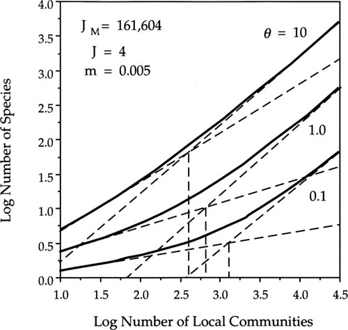
Figures 6.17 and 6.18 illustrate how the species-area curves at large spatial scales and the correlation length L are controlled by the fundamental biodiversity number θ and by the dispersal parameter m. In figure 6.17 I have varied θ over two orders of magnitude from 0.1 to 10, holding m constant at 0.005. From figures 6.14 and 6.15, we would predict that increasing θ for a fixed value of m will raise the local species richness (α-diversity) as well as the slope (z value, β-diversity) of the species-area curve at intermediate spatial scales (figs. 6.17, 6.18). As θ increases and the species-area slope steepens, the inflection point in the curve becomes less pronounced because the difference in slope above and below the inflection point becomes less and less. As θ increases, the upper and especially the lower tangent lines increase in slope. In figure 6.17, the upper tangent line increases from z = 0.886 for θ = 0.1 to z = 0.961 for θ = 10.0. The correlation length L decreases with increasing θ for a given value of m. This is because increasing the speciation rate increases the number of species in the metacommunity, which reduces the mean size of populations and their geographic ranges because of the zero-sum rule. However, the correlation length increases with increasing dispersal rate m for a given value of θ. Increasing dispersal distributes common metacommunity species more widely, and couples the dynamics of local communities more broadly geographically, enlarging average range sizes. Increasing the dispersal rate also reduces total metacommunity diversity, a phenomenon that will be examined more fully in chapter 7.
FIG. 6.17. Species-area relationships at large spatial scale for a metacommunity of 201 × 201 local communities, J = 4. Curves are drawn for θ = 0.1, 1.0, and 10.0, for a low migration rate (m = 0.005). The correlation length L decreases with increasing θ for small m. Mean of one hundred simulation runs.
FIG. 6.18. Species-area relationships at large spatial scale for a metacommunity of 201× 201 local communities, J = 4. Curves are drawn for θ = 0.1, 1.0, and 10.0, for a high migration rate (m = 0.5). The correlation length L increases with decreasing θ for large m. Mean of one hundred simulation runs.
The correlation length L is a really important concept and number because it measures and defines the natural length scale of a biogeographic process over which metacommunity events are dynamically and evolutionarily connected. It is an especially important number for conservation biology because it quantifies the size and region within which observed metacommunity biodiversity evolves, lives, and dies. Thus, the unified theory assumes that, besides relative abundance distributions, species-area curves also contain information about both the fundamental biodiversity number and mean dispersal rates throughout the metacommunity. Although the slope of the species-area curve does not functionally determine the values θ and m, z does constrain θ and m to lie along a single isocline in θ-m parameter space (fig. 6.15). Conversely, knowing θ and m, according to the unified neutral theory, is sufficient to predict the slope of the species-area power law relationship expected on intermediate spatial scales.
The theory developed here for species-area curves makes the assumption that speciation rate is independent of dispersal rate. In general, one would expect speciation and migration rates to be inversely related (Mayr 1963, Slatkin 1977, 1980). High rates of dispersal should promote panmixis and therefore inhibit the speciation rate, at least for some modes of speciation. As we have seen, however, even assuming no interaction between dispersal and speciation, high rates of dispersal lead to lower slopes of species-area curves. A negative effect of dispersal on speciation would reduce the slopes of species-area curves still further. In the absence of quantitative data on the effect of dispersal on speciation rate, there is little beyond this qualitative statement that can be said here.
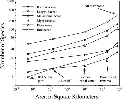
Before I conclude this chapter, it is useful to illustrate the application of the theory to interpreting species-area curves. My example consists of species-area relationships in twenty seven families of Panamanian trees and shrubs, compiled from regional checklists in the Flora of Panamá (D’Arcy 1987). Species-area curves were constructed for trees and shrubs achieving stem diameters > 1 cm dbh. The areas within which nested species counts were made ranged from the 50 ha plot (0.5 km2) on Barro Colorado Island (BCI) at the low end, to all of BCI (15 km2), to the area of the former Canal Zone (103 km2), to the province of Panama (2· 104 km2), and finally to the entire country of Panama (7.5 · 104 km2). From these data I computed the z values of the species-area curves for each family. Figure 6.19 presents the species-area curves for a representative sample of 6 families. Three of these are primarily families of midstory, canopy, or emergent trees in Panama (Bombacaceae, Myristicaceae, and Lecythidaceae), and three other families are generally shrubs or understory trees (Melastomataceae, Piperaceae, and Rubiaceae). I calculated the z values for the log-log linear portions of the curves, up to the area of the former Canal Zone.
Of the six sample families, the lowest z value occurred in the family Bombacaceae (z = 0.097), a family of mainly emergent, late secondary heliophilic species with small, wind- or bat-dispersed seeds (Croat 1978). Steeper curves were found in families of understory trees and shrubs (Melastomataceae, z = 0.201, Piperaceae, z = 0.195, and Rubiaceae, z = 0.190). Even steeper curves were found in the New World nutmeg family, Myristicaceae (z = 0.215) and in the brazilnut family, Lecythidaceae (z = 0.262). Myristicacs have large arillate, seeds dispersed by large frugivorous birds, but seldom far. Lecythidacs are a family of mainly midstory tree species, but with relatively poor seed dispersal. They have very heavy fruits containing large seeds that are eaten and scatter-hoarded by ground-foraging mammals. The diversity of species-area curves in figure 6.19 implies that the assumption of identical per capita dispersal and speciation probabilities among these families has been violated. However, as it turns out, the unified theory is quite robust to violations of this assumption, so long as the zero-sum rule still applies (chapter 10).
FIG. 6.19. Species-area curves for trees and shrubs > 1 cm dbh in 6 plant families in Panama, over a range of spatial scales from the 50 ha plot on BCI to all of Panama. Note the log-log linear curves at intermediate scales, up to the area of the former Canal Zone. It is suggestive and perhaps significant that all of the cures show a sudden upturn at approximately the same spatial scale, which corresponds to a correlation length of 70—130 km, the average width of the isthmus of Panama.
While it is perhaps not surprising that each of these plant families shows a unique species-area curve, what is striking is that all show a sudden upturn at about the same spatial scale (fig. 6.19). If we take this as a rough estimate of the correlation length, then it ranges from about 70 km to 130 km, approximately the average width of the isthmus of Panama. All but two of the twenty seven plant families show a similar inflection point. This strongly suggests that biogeographic processes of origination, dispersal, and extinction in the isthmus of Panama are constrained in some fashion by the fact that they are taking place on a long, narrow piece of land. This suggests that the geometry of a particular biogeographic area may override the theoretical expectations that each species-area curve should have its own intrinsic and endogenously generated correlation length.
We can estimate the approximate correlation lengths of the six Panamanian tree and shrub families in figure 6.19. All six curves are log-log linear up to a spatial scale of approximately 103 km2, the area of the former Canal Zone. Then all begin to bend upwards, more or less at the same spatial scale, steepening to the area of the province of Panama, and steepening once again to the area of the entire country of Panama. Note that the curves, although becoming steeper, do not attain a slope of unity by the time all of Panama has been sampled.
I used the smallest three sample areas for each family to estimate the lower tangent line, and the two largest sample areas—the province of Panama and all of Panama—to estimate the upper tangent line. These yielded the following L2 and correlation length L values for each of the six families: Bombacaceae: L2 = 11,000 km2, L = 105 km; Lecythidaceae: L2 = 16,000 km2, L = 126 km; Melastomataceae: L2 = 5,700 km2, L = 75 km; Myristicaceae: L2 = 7,000 km2, L = 84 km; Piperaceae: L2 = 6,800 km2, L = 82 km; and Rubiaceae: L2 = 4,600 km2, L = 68 km. It is interesting that all of the estimated correlation lengths are small and relatively similar, varying only over about a 2 fold range, from 68 km to 126 km. Also, the three plant families that are primarily understory shrubs and treelets (Melastomataceae, Piperaceae, and Rubiaceae) had the smallest correlation lengths.
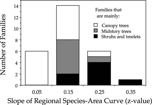
The historical, ecological, and evolutionary explanations for the variation in species-area curves among Panamanian tree and shrub families are currently unknown. Speciation rate aside, however, one might expect that dispersal rates would be affected by plant growth form. Canopy trees might be expected to disperse seeds on average farther and faster than small-stature understory shrubs or herbs. Therefore, plant families that are comprised mainly of canopy or emergent tree species might be expected to have shallower species-area curves than families comprised mainly of shrubs or herbs. The species-area data for the twenty seven Panamanian tree and shrub families show generally good agreement with this prediction (fig. 6.20). On intermediate spatial scales, families comprised mainly or exclusively of canopy or emergent tree species exhibited species-area curves having consistently lower z values than families comprised mainly of understory trees, treelets, or shrubs.
FIG. 6.20. Relationship between the characteristic stature of species in 27 tropical tree and shrub families in the flora of Panama and the slope (z-value) of the Arrhenius log-log linear species-area curves for families at intermediate spatial scales in Panama. Families comprised mainly of small-stature species have steeper species-area curves than families of large-stature species.
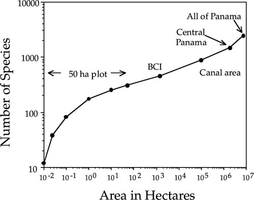
When we examine the species-area curve for the complete native tree and shrub flora of Panama, we see a similar upturn in the species-area curve at about the same spatial scale (fig. 6.21). Drawing the upper and lower tangents to the species-area curve yields an L2 of 4300 km2, and a correlation length of 65.6 km, which once again is commensurate with the average width of the Panamanian isthmus. We can also estimate the correlation length for the vascular plant flora of the world from fig. 6.3 (Shmida and Wilson 1985). The value of the squared correlation length is approximately 7 · 1011 m2, yielding an estimated correlation length L of 8.4 · 105 m, or 837 km. For the world’s avifauna, the squared correlation length is approximately 2.5·106 km2 (fig. 6.2), yielding a correlation length L of 1585 km.
FIG. 6.21. Species-area curve for the entire native tree and shrub of Panama, over a range of spatial scales from 10−2 ha (a 10× 10m quadrat within the 50 ha BCI plot) to all of Panama. In Panama, the range of intermediate spatial scales over which the log-log linear Arrhenius relationship applies is approximately from 1 ha to 105 ha, suggesting that the mean correlation length for the Panamanian tree flora lies somewhere in the range of 30—300 km. Data extracted from D’Arcy (1987). Note similarity in shape to Shmida and Wilson’s (1985) species-area curve for the world’s flowering plants (fig. 6.3).
1. When species-area curves are plotted from local to global scales, they are triphasic, indicating that different scaling rules apply on different spatial scales. As a result, the Arrhenius relationship, a linear log-log species-area power law—which implies self-similarity in the intermediate scaling region for which it applies—does not work at small and very large spatial scales.
2. The unified theory asserts that these triphasic species-area curves are the spatial manifestation of the steady state of a dynamical, neutral speciation-dispersal-extinction process playing out on the metacommunity landscape. The theory explains the triphasic nature of species-area curves without resorting to niche-assembly hypotheses.
3. On local spatial scales, species-area curves are sensitive to the local relative abundance of species and are curvilinear on a log-log plot.
4. On regional spatial scales, the theory always predict’s linear log-log species area curves whose slopes (z values) depend on the fundamental biodiversity number θ and m, i.e., on the relative rates of speciation and dispersal across the metacommunity landscape.
5. At large spatial scales, the neutral theory predicts the existence of a natural length scale, the correlation length L, which defines the mean size of evolutionary-biogeographic units on the metacommunity landscape; L is a function of θ and m.
6. As spatial sampling scales exceed L, the slope of the log-log species-area curve steepens toward unity as evolutionary-biogeographic processes on regional scales become increasingly uncoupled and dynamically uncorrelated with one another.
7. The spatially explicit theory needed for species-area relationships differs from the spatially implicit theory for the classical island-mainland problem posed by MacArthur and Wilson in that both the fundamental biodiversity number θ and the dispersal rate m must be specified.