The theory of island biogeography has been criticized in recent years for failing to take into account the fragmented nature of populations and the habitats that they occupy (e.g., Hanski and Simberloff 1997). Perhaps this criticism has some validity when applied to the classical island-mainland problem posed in the original theory. But in fairness, MacArthur and Wilson did consider the more complex problem of the biogeography of archipelagos of islands or habitats. Since their monograph appeared more than 30 years ago, great strides have been made in understanding and mathematically characterizing complex landscapes (Mandelbrot 1982, Milne 1997, Ritchie 1997, Ritchie and Olff 1999). Indeed, the whole field of fractal geometry did not exist then (Gleick 1987); but there is no reason in principle why the theory cannot encompass fractal landscapes and metapopulation biology. Probably the most important reason for incorporating the metapopulation perspective is the practice of conservation biology. Although natural habitats have always been patchy, the anthropogenic destruction of natural habitats has greatly worsened the problem of habitat fragmentation (Tilman et al. 1994), and fragmentation is a fact of life that is here to stay.
How are the conclusions we have reached in previous chapters affected by habitat fragmentation? How does the metacommunity equilibrium distribution of relative species abundance change on a fragmented landscape? How are the expected times to extinction of individual species affected by habitat fragmentation under the neutral theory? A full examination of these questions is beyond the scope of present work, and lies in the future. However, there are a number of initial questions we can explore with the existing theory. I first consider a single-species population and ask: Under ecological drift and random dispersal, what is the probability that a species is present or absent from a local community, as a function of local community size, the probability of immigration, and the metacommunity relative abundance of the species? Then I consider an archipelago of islands or habitats and ask: What is the covariance of abundance of the ith species among islands or habitat patches? Finally, I consider metacommunities and ask: How is biodiversity explicitly spatially distributed on a continuous metacommunity landscape?
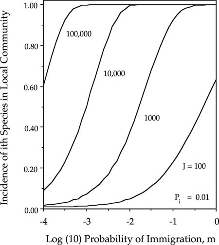
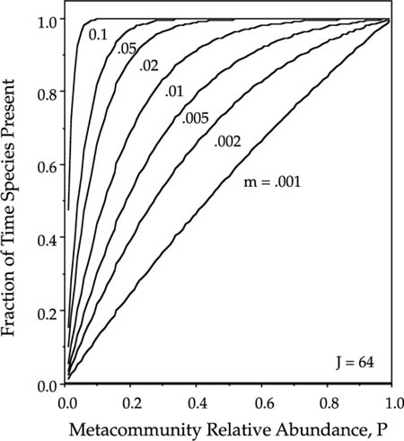
One of the most important questions for the conservation of particular focal species is the probability that the species is present in a given patch. This is formally equivalent to the proportion of time that the species occupies the habitat patch. We can study such incidence functions from the theory developed in chapter 4 for the dynamics of single species undergoing zero-sum ecological drift. The incidence function specifies the equilibrium fraction of time that the ith species will be present in the local community, which is given by the sum of the elements of the eigenvector Ψ(n) for Ni ≥ 1 (see chapter 4). Increasing both m and Pi increases the incidence of the ith species in the local community (fig. 7.1). An important conclusion from figure 7.1 is that it does not take a very high rate of immigration or a high metacommunity relative abundance of the focal species to have a high probability of being present in a local community. However, obviously the immigration rate must be nonzero, and there must be a metacommunity from which immigrants can come. This result is from the implicit space version of the theory (see Chapters 4 and 5), and it assumes a very stable metacommunity from which immigrants are drawn, stabilized by the law of large numbers.
FIG. 7.1. Equilibrium incidence functions for the ith species in an ergodic community undergoing zero-sum drift, as a function of probability of immigration m, and metacommunity relative abundance Pi for a local community of size J = 64.
Increasing the size of patches also has a large effect on the probability that a species will be present in the given patch or local community (fig. 7.2). For example, if the patch or local community size J is 105, then an immigration rate of 10−3 will maintain the presence of a rare metacommunity species (1% of the metacommunity) essentially 100% of the time. Larger communities also lower the extinction rate. This is because larger communities allow larger population sizes to develop, which in turn delays the inevitable local extinction. This is the primary insight that led MacArthur and Wilson (1967) to draw extinction rate curves as a function of island size in their graphical model of island biogeography. The smaller the community size or habitat patch of individuals, the more likely a species is to be absent and the more variable the species composition of the community will be. Also, the more isolated a community is, the more likely a given species is to be absent, in accordance with MacArthur and Wilson’s theory.
FIG. 7.2. Equilibrium incidence functions for the ith species in an ergodic community undergoing zero-sum drift, as a function of probability of immigration m, and a metacommunity relative abundance Pi = 0.01, for four orders of magnitude variation in local community of size.
Another perspective is obtained from calculating the persistence function. The persistence function gives the mean passage time of a species between abundance i and abundance j. A particularly important persistence function is that which characterizes the mean passage time between colonization and extinction events of a species in the local community or island. The shortest passage times to extinction will be found in species with lowest abundances, which will include most recent colonists. However, if a species manages to become common in the community, its expected passage time to extinction will increase. The mean persistence times can be calculated for the ergodic community as follows. For any ergodic process, which is defined as one in which every state is ultimately reachable from every other state, there exists a matrix T = {tij} of the mean number of steps to reach abundance j for the first time, starting in abundance i. Matrix T is given by
T = W − Wdg
W = {I − E + CEdg}D,
where I is the identity matrix, E is the fundamental matrix of the ergodic process, C is a matrix whose entries are all unity, Wdg and Edg are matrices with the same elements on the principal diagonal as matrices W and E, respectively, and zeros elsewhere, and D is a diagonal matrix with each element on the principal diagonal equal to 1/Ψj. The fundamental matrix E is given by
E = {I − B + Ψ}−1,
where B is the matrix of transition probabilities for the ergodic process, and Ψ is a matrix whose elements are ψi across each row (see chapter 4).
It is instructive to consider again our simplest ergodic community, when J = 1. The mean passage time to extinction for the resident species is easily found from the above equations to be
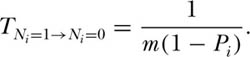
This demonstrates that persistence time in the patch or local community is inversely related to the immigration rate m and also inversely related to the collective relative abundance of all species other than species i in the metacommunity. As the ith species increases in metacommunity relative abundance toward monodominance (i.e., as Pi → 1), the persistence of the ith species tends toward permanent occupancy (TNi=1 → ∞) of any given local site. Also note that the site is permanently occupied by species i (i.e., by whatever species is initially present) if there is no immigration (m = 0). The inverse relationship between persistence and immigration rate may seem counterintuitive. However, recall that the immigration rate in MacArthur and Wilson’s original model applied to all species—not just a given focal species. Therefore, increasing the immigration rate has the effect of increasing the rate of species turnover in a patch or local community, displacing resident species by other species immigrating into the patch from the metacommunity.
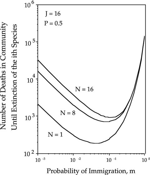
The mean passage time to extinction is the shortest for Ni = 1. For initial abundances Ni > 1, the mean passage times become longer and the persistence functions become more complex in communities of size J > 1. Figure 7.3 shows the case of a patch or local community of size J = 16, and the persistence functions for Ni = 1, J/2, and J. The persistence functions are now U-shaped for J > 1. At very low and very high rates of immigration, the persistence times are longer than at intermediate rates of immigration. At low rates of immigration, there is no force of immigration to increase the turnover rate of species in the patch. At very high rates of species immigration, the immigration provides a subsidy of the species in the patch, and this subsidy delays the local extinction of the ith species. This is the unified theory’s formal confirmation of the “rescue effect” postulated by Brown and Kodric Brown (1977). The parallels with the absorbing case discussed in chapter 4 are obvious.
FIG. 7.3. Persistence fuctions (number of deaths in the patch or local community until extinction) of the ith species in the patch, as a function of the probability m and the initial population size, Ni, in a patch of size 16, and for a focal species with a relative abundance in the metacommunity Pi of 0.5.
As in the absorbing case, the length of time to extinction rises rapidly with increasing community size and with initial abundance. However, the possibility of immigration from the metacommunity adds richer behavior to the persistence functions.
The variances of the persistence functions can also be calculated. The matrix of variances in time to reach abundance j starting at abundance i is given by
Var(T) = W{2Edg D − 1} + 2{EW – C(EW)dg}.
Among the elements of Var(T) are the variances in passage times to extinction from any starting abundance. As in the absorbing case (chapter 4), the time to local extinction in the ergodic community is approximately gamma distributed.
I now consider the covariance of the abundance of the ith species between two discrete habitat patches, islands, or local communities. Imagine an archipelago of habitat patches or islands and let this archipelago be bathed in a background immigration rate. Now consider two islands, and imagine that they are dynamically coupled both through the background metacommunity immigration, and through the exchange of migrants specifically between the two islands or habitat patches. The expected total abundance of the ith species in the two equal-sized habitat patches or islands of size J is simply 2JPi. But how does the abundance of the ith species covary in these habitat patches as a function of reciprocal migration? Presumably, local communities that are immediately adjacent to one another will be more similar in abundance of the ith species than communities separated by greater distance. These local communities are dynamically coupled to one another, and the strength of this coupling depends on the rate of exchange of migrants, the size of the local communities, as well as the fundamental biodiversity number. This covariance in the ith species among two local communities can be studied analytically.
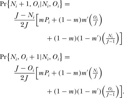
Consider the dynamics of the ith species in the context of the ergodic community studied in chapter 4. Now, however, let us consider the coupled dynamics of two local communities that exchange migrants per birth with probability m′, and let m once again be the probability that either local community receives an immigrant from the metacommunity in which they are imbedded. Note that m′ may be larger than m, but it will often be smaller than m because the metacommunity typically is a much larger source area than a single other local community or another island in an archipelago, and so it has a higher “mass effect” (Shmida and Ellner 1984). Let Ni and Oi be the abundances of the ith species in the two local communities, respectively, each of which is of size J. Assume D = 1 for simplicity. We can now write down the transition probabilities for changes in the joint abundance of the ith species:
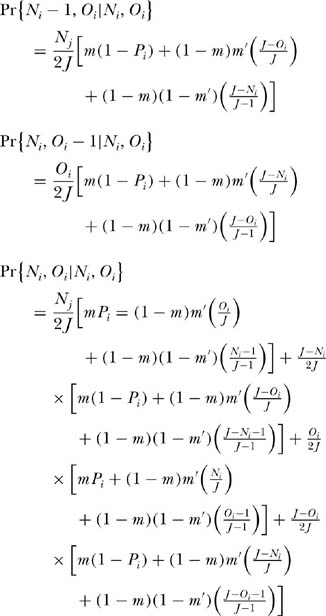
Note that these equations differ from those for the single ergodic community in having an additional term for immigration from the other local community. Also note that each probability is multiplied by one-half. This is because of the condition that D = 1 and the single death per death-birth cycle occurs in one or the other local community with equal probability, 0.5.
We can once again compute the eigenvector for this system of equations. For the simplest case of two local communities of size J = 1, the eigenvector is
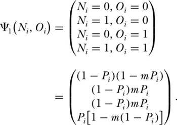
When two local communities are considered jointly, the J = 1 case is no longer independent of the probability of immigration from the metacommunity, m, as it was in chapter 4. However, the J = 1 case is independent of the probability of migrants from one local community to the other m′. Note that as m → 1, Pr{0, 0} → (1 − Pi)2 and Pr{1, 1} →  . As Pi → 1, Pr{0, 0} → 0 and Pr{1, 1} → 1; conversely, as metacommunity abundance Pi → 0, Pr{0, 0} → 1 and Pr{1, 1} → 0.
The eigenvector for arbitrary J > 1 is algebraically extremely messy, but it is easy to compute exactly. From this eigenvector, we can directly calculate the covariance of the abundance of the ith species in the two local communities. The expected abundance in each local community is identical to the expectation derived in chapter 4 in the single local community case: E{Ni} = E{Oi} = JPi. Therefore, the covariance in abundance of the ith species is
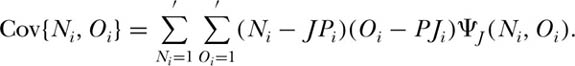
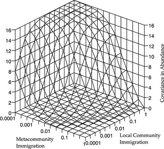
Figure 7.4 illustrates the functional dependence of the covariance in the abundance of the ith species on the probabilities of immigration from the source metacommunity m, and from the other local community m′, for a local community size J = 8. The covariance exhibits contrasting dependence on m vs. m′. Increasing the migration rate from the metacommunity decreases local community covariance, whereas increasing the reciprocal migration rate between the local communities increases their covariance. The covariance between local communities is zero when m = 1 and m′ = 0. Conversely, the local communities maximally covary when m → 0 and m′ = 1, in which case the limiting maximal covariance is (JPi)2.
We can now answer the question of how the abundances of the ith species in two local communities will covary as a function of their dynamic coupling through reciprocal migration. We can measure distance between local communities of equal size J in units of  . In the last chapter we noted that, on local spatial scales, the probability of immigration to a local community from the metacommunity will fall off approximately as some power function of local community size, m(J) = J−ω. Assuming that the background immigration rate m from the metacommunity is not affected by varying the spatial separation of the two local communities, and because J increases linearly with area, then we simply compute the covariance as a function of m′ = n(J/ρ)−ω′/2, where ω′ is empirically measured, and n = 1, 2, 3, . . . .
FIG. 7.4. Covariance of the abundance of the ith species in two habitat patches or islands as a function of the probability of immigration from the metacommunity, m, and from the other local community, m′. In this example, local community size J = 8 and metacommunity abundance Pi = 0.5.
The preceding analysis is most appropriate for a fragmented landscape or an archipelago of islands where one can treat space implicitly. I have not worked out the covariance when the two local communities are imbedded in a landscape in an explicitly spatial model. In this case, there will be distributed effects of dispersal from near and far communities, and the covariance function will be considerably more complex than the case computed here. This is another example of the many interesting theoretical problems in the neutral theory that remain for the future.
I turn now to a consideration of the distribution of total biodiversity on the metacommunity landscape. Although there are few analytical results for the explicit spatial case, the results of many simulations lead to a number of important qualitative generalizations that are consistent with the analytical results presented in chapters 4 through 6. As we have seen in chapter 6, the steady-state species-area relationship is controlled by the fundamental biodiversity number θ and by the probability of dispersal m. This implies that speciation and dispersal limitation (m < 1) will affect the distribution and maintenance of biodiversity on local to regional scales under zero-sum ecological drift, and the spatial autocorrelation of community species composition. We can illustrate several of the most important generalizations with the results of a numerical experiment, simulating a metacommunity consisting of 101 × 101 local communities, each of size J = 16. I initialized diversity at one individual per species, and ran simulations for 100,000 birth-death cycles with four deaths per local community per cycle, resulting in 25,000 complete turnovers of the metacommunity. In this example, the fundamental biodiversity number θ was set at 14, a reasonable value, say, for a southern temperate forest. Let dispersal in one time step be restricted to the Moore neighborhood (chapter 6) of any given local community.
Now consider two cases: case I, in which migration rates are very low (m = 0.005) and local communities are quite isolated from one another; and case II in which migration rates between neighboring communities are very high (m = 0.5) and local communities are quite connected by dispersal. In case II, one out of every two births is an immigrant, whereas in case I, immigration accounts for only one out of every two hundred births.
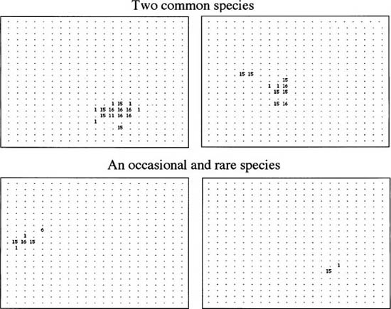
What do we predict about the spatial structure of species populations in the metacommunity from the neutral theory? Recall from the analytical results of chapter 4 that under severe dispersal limitation, a focal species is expected to spend most of the time either locally extinct or, less often, monodominant. This implies that local communities will become less diverse, lose species, and show increased dominance under low immigration rates and greater isolation. If dispersal rates are low, then some species or other gets carried by ecological drift to high local abundance and potentially monodominance. Conversely, if the dispersal rates are high, then local communities will have more species and monodominance will be rare or absent. In figure 7.5 I show sample results for case I (low dispersal rate), and I have plotted the distributions of four representative species in a block of 21 × 21 local communities in the center of a 101 × 101 metacommunity: two common species, a species of intermediate abundance, and a rare species.
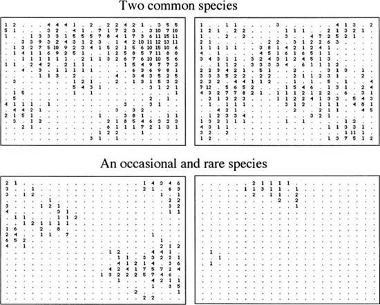
Under case I, when dispersal is extremely limited, a tile-like mosaic pattern becomes apparent (fig. 7.5). Common and rare species alike show a strong tendency toward monodominance in their respective patches. Thus, low rates of migration strongly reduce local community species richness and increase local dominance. Note that these monodominant local communities tend to have occasional satellite individuals in adjacent communities, but rarely more than one or two individuals at a time. Thus, as predicted, strong dispersal limitation reduces local community species richness and increases local community dominance. This effect becomes stronger as m → 0. The spatial distributions of species under case II are completely different from case I (fig. 7.6). When local communities are strongly coupled dynamically through high rates of dispersal, the tile-like mosaic of monodominant species completely disappears. In its place, we have much more amorphous and diffuse spatial distributions, and local community species richness is higher while dominance is lower. Because this is a stochastic equilibrium, the individual species distributions on the metacommunity landscape are not static but continue to move about as species come and go. Note also that metacommunity populations of individual species may become fragmented into isolated demes, and look and behave like metapopulations. It is interesting that such fragmentation arises more frequently when dispersal rates are high rather than low.
FIG. 7.5. case I: Local communities are very isolated (m = 0.005). Typical species distribution maps at steady-state under spatially explicit ecological drift in the central block of 21 × 21 local communities each of size J = 16. The numbers in the grids are the local abundances of the given species. Fundamental biodiverity number in the grids are the local abundances of the given species. Fundamental biodiversity number θ = 14. The species in the top two panels are maps of two common species; the bottom two panels are an occasional (left) and a rare species (right), respectively. Note that all species form patches of partial to complete local monodominance producing a mosaic metacommunity. Total metacommunity size is 101 × 101 local communities.
FIG. 7.6. case II: Local communities are highly coupled by migration (m = 0.5). Typical species distribution maps at steady-state under spatially explicit ecological drift in the central block of 21 × 21 local communities each of size J = 16. Numbers in the grids are the local abundances of the given species. Fundamental biodiversity number θ = 14. The species in the top two panels are maps of two common species; the bottom two panels are an occasional (left) and a rare species (right), respectively. Note that species are much more diffuse in dispersion patten, and much more intermingled in local communities than in case I. Total metacommunity size is 101 × 101 local communities.
These simulated spatial patterns are only caricatures of the much more complex patterns that would be found in actual natural communities, but they are nevertheless sufficient to make the following very important general point. Under low rates of dispersal, species are found at higher local abundance in patches of lower local species richness. Conversely, under high rates of dispersal, species occur at lower abundance in local communities having higher species richness.
This means that there is a change in the distribution of α (local) and β (regional) diversity with a change in the dispersal rate (fig. 7.7). High rates of dispersal bring more regional diversity to the local community, but a consequence is that abundant and widespread metacommunity species drive rare and local species extinct from the metacommunity. The result is that total metacommunity biodiversity is reduced by high dispersal rates. Conversely, low rates of dispersal let many rare local “endemics” survive in small pockets of high abundance, so that total metacommunity biodiversity is increased. Low dispersal rates mean that ecological drift has adequate time between dispersal events or carry a species to high local abundance. Because dispersal is infrequent, there is little force of immigration to break up these local pockets of high abundance or monodominance. As was shown in chapter 4, monodominant species in local communities take much longer to drift to local extinction than less abundant species in the local community. Thus, the general result is that under high rates of dispersal, local diversity is high but metacommunity diversity is low; whereas under low rates of dispersal, local diversity is low but metacommunity diversity is high.
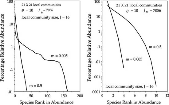
Note in figure 7.7 that the dominance-diversity curve for the metacommunity in the dispersal-limited case has somewhat of a staircase-like appearance. This is due to the high frequency of species having abundances that are multiples of the local community size J, which in this case was set to 16. Thus, there are greater numbers of species with abundances of 16, 32, 48, etc., than would otherwise be expected without such frequent local monodominance. This staircase is in essence a modeling artifact of having to simulate very small discrete community sizes in the computer. With continuous intergradations of local communities, the frequency of perfect local monodominance becomes very small, and this staircase appearance disappears. One would not expect to see this effect in spatially continuous ecological communities in nature.
FIG. 7.7. Comparison of the steady-state dominance-diversity curves that arise under strong dispersal limitation (case I: m = 0.005), and under strong dispersal coupling (case II, m = 0.5) among local communities of size J = 16. Left: Metacommunity dominance-diversity. Right: Local community dominance diversity. Dominance-diversity curves were computed for the central block of 21 × 21 local communities in a metacommunity of 101 × 101 local communities after 100,000 birth-death cycles, and four deaths in each local community per cycle.
Let us now consider the question of how the similarity of communities changes with distance across the metacommunity landscape. Many ecological and evolutionary processes will produce a loss in similarity between two ecological communities with increasing separation distance. Under niche-assembly theory, distance decay is predicted to result from species turnover along local and regional environmental gradients or among habitats. In nature, habitats are often patchy and recurrent, so that the decay of community similarity with distance may frequently not be smooth. However, the neutral theory also predicts a decay in community similarity with distance, and it does so on completely homogeneous landscapes. Indeed, perhaps the smoothest decay in similarity with distance should be predicted by neutrality because no other forces are operating besides ecological drift, random dispersal, and random speciation. The reason for the decay in similarity is that large steady-state differences exist in the metacommunity abundances of species, coupled with dispersal limitation that is increasingly severe in ever rarer species. The steady-state distribution of metacommunity species abundance and the level of dispersal limitation are dictated by the fundamental biodiversity number θ and by the dispersal rate m. We have already seen that the neutral theory predicts species-area relationships chapter 6), so it should come as no surprise that the theory also predicts the distance decay in similarity in communities, which in a sense is simply the inverse problem.
In an excellent analysis of the distance decay of similarity in biogeography and ecology, Nekola and White (1999) analyzed data on the decay of similarity in several plant metacommunities. Perhaps the most relevant of their datasets for testing the neutral theory (because of its relative homogeneity) is one on boreal upland white spruce forests, a dataset collected by LaRoi (1967) and LaRoi and Stringer (1976). The dataset consisted of species lists in thirty-four 9 ha plots over a 6000 km transcontinental transect from Newfoundland to Alaska. These plots collectively contained 561 species of vascular plants. To measure similarity in communities, Nekola and White used Jaccard’s Index (Mueller-Dombois and Ellenberg 1974), which is probably the most widely used and familiar index of similarity. They used a Mantel’s test with 10,000 replications to obtain bootstrap estimates of the significance of their statistical models (Manly 1991).
With this and other datasets, Nekola and White (1999) were able to ask a number of fundamental questions, including the following. First, what is the functional form of the distance-decay curve? Second, does this curve depend on what component of the plant community is considered, such as trees, shrubs, or herbs? Third, do species of differing metacommunity abundance contribute differentially to the decay curve? Fourth, is there evidence of involvement of mode of dispersal in the rate of distance decay, i.e., do better dispersing taxa have slower rates of distance decay?
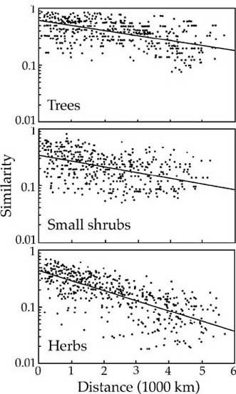
The similarity decay curves for trees, small shrubs, and herbs in upland white spruce forests across Canada and Alaska are shown in figure 7.8 over the 6000 km range. In answer to question 1, Nekola and White (1999) found that these decay curves were all fit best by simple negative exponential functions. In answer to question 2, the steepness of these decay curves was a function of plant growth form. It was shallowest for trees, and became progressively steeper the smaller the plant growth form (fig. 7.8). In answer to question 3, the component of abundant and widespread species had shallower decay curves than the component consisting of species of intermediate abundance (not illustrated). However, the rare-species component also showed very little decay in similarity because it was already maximally dissimilar due to the generally very local distribution of rare species. Finally, in answer to question 4, mode of dispersal did influence the decay of similarity. Animal-dispersed, fleshy fruited species had slower rates of decay than wind- or spore-dispersed species. These results are entirely congruent with the results presented in chapter 6 on the species-area relationships for the tree flora of Panama.
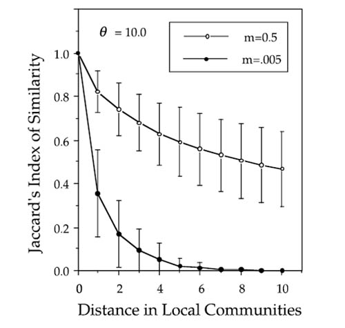
The neutral theory’s qualitative predictions are completely consistent with Nekola and White’s results, but they differ slightly in the predicted functional form of the decay curve because the expected curves are not perfect exponentials. And they should not be for the very reasons given by Nekola and White (1999): namely, that communities consist of mixtures of widespread and abundant metacommunity species, and of rarer and more local species whose distance decay is steeper. This heterogeneity will produce somewhat rounded distance-decay curves that are compound exponential, with a different exponent for each added species abundance class of the community. Typical curves that one obtains from the neutral theory are shown in an arithmetic plot in figure 7.9, and in a semilog plot in figure 7.10. They start more steeply because they are dominated by the turnover of rare and occasional species that are not widespread. However, as more and more of the local species drop out, the species that remain are the widespread and abundant species, so the distance-decay curve will begin to slow down and have a shallower and shallower slope.
FIG. 7.8. Distance decay in Jaccard’s Index of Similarity for three components of upland white spruce forest from Newfoundland to Alaska over nearly 6000 km. Three components of the vascular plant community are sown: trees (top), small shrubs (middle) and herbs (bottom). Slopes of semilog plots are as follows: trees, −0. 19; small shrubs, −0. 28; and herbs, −0. 40 After Nekola and White (1999).
FIG. 7.9. Distance decay in community similarity according to Jaccard’s Index. Decay in similarity is much faster for low rates than for high rates of dispersal. These curves were averages over one hundred simulations of a 101 × 101 metacommunity, with a local community size of J = 8 and a fundamental biodiversity number θ of 10. The curves are drawn for the central 21 × 21 community region in the middle of the metacommunity. Error bars are one standard deviation of the mean. These curves appear exponential on an arithmetic plot, but they are actually compound exponential. See figure 7.10.
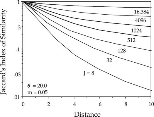
FIG. 7.10. Semilog plot of the distance decay of Jaccard’s Index of Similarity, revealing the compound exponential nature of the decay curves. The curvilinearity is easier to detect when using a small sampling “grain size” or local community (i.e., small J) rather than large J, and when the decay curves are plotted semilogarithmically. Distance is measured in number of local communations.
Note that the distance-decay curve is strongly influenced by the mean dispersal rate over the metacommunity (fig. 7.9). High dispersal rates prevent differentiation of local communities through ecological drift. Conversely, low dispersal rates allow much more local differentiation of community composition, and the distance-decay curves are much steeper. Once again, this is completely consistent with the analytical results of chapter 4.
The curvilinearity of the distance decay is more obvious for small J and when the decay curves are plotted semilogarithmically. The degree of curvilinearity will depend on the degree of differentiation of relative species abundance in the metacommunity, which depends on the fundamental biodiversity number θ and on the dispersal rate m. This effect is seen in figure 7.10, in which I have varied J, the size of the local community as the sampling unit. The compound nature of the exponential distance decay curve will be harder to detect if the local community size is large. This corresponds to choosing a large spatial sampling unit or “grain size” sensu Palmer and White (1994). This effect happens because most of distance decay in similarity of the rare and local species will occur rapidly at shorter distances. Given the scatter in the data on distance-decay curves such as those shown in figure 7.9, and given the relatively slight curvature expected on these spatial scales, it may be difficult to detect the predicted curvilinearity in the distance-decay relationship. However, the very fact that shallower slopes were obtained for widespread taxa than for taxa of intermediate frequency indicates that this curvilinearity must be present in the datasets used by Nekola and white (1999).
The effects of dispersal on α and β diversity have major implications for conservation strategies. Changes in the mean dispersal rate cause changes in the spatial distribution of total biodiversity and the degree of local endemism across the metacommunity landscape. In recent papers, Harte and Kinzig (1997) and Harte et al. (1999) point out that the species-area curve for endemics has the same functional form as total species-area curves on intermediate spatial scales, i.e., S = cAz, but the exponent z is much steeper for endemics than for total species richness. This phenomenon is predicted by the unified theory because a low dispersal rate has the effect of making species locally more abundant but also rarer and endemic to smaller regions of the metacommunity landscape as a whole. Thus, species-area curves are significantly steeper when dispersal limitation is greater, consistent with our results from the preceding chapter.
These results also have important implications for the twenty-five-year-old debate about reserve design, and the wisdom of having one large reserve versus many small scattered reserves (Diamond and May 1975, Wright and Hubbell 1983, Burkey 1995). From the perspective of the unified theory, this question cannot be resolved definitively without understanding the degree of dispersal limitation affecting the metacommunity and how dispersal limitation will be affected by fragmentation of the landscape. The message from the theory, therefore, is that we need to gather much better and more extensive information about dispersal ability and actual movements of species over the metacommunity landscape. Qualitatively we can say, however, that the more dispersal limited or fragmented the metacommunity, the more likely that a multiple reserve design will be necessary to save local endemics. This point was also stressed by Harte and Kinzig (1997).
Tilman et al. (1997) discussed the trade-off between dispersal limitation and competitive ability in this context. They argued that good competitors, which are species capable of holding onto sites but are generally not good dispersers, will suffer the most from fragmentation of the landscape because their movement will be more affected by fragmentation than the movement of good dispersers. Species in the unified theory do not exhibit this trade-off, and so the present neutral theory does not make such a prediction. However, it does predict that species that are common and widespread throughout the metacommunity prior to fragmentation will also be the most resistant to the effects of fragmentation. Thus, the unified theory asserts that the most critical factor determining the long-term survival of a species is its metacommunity abundance and distribution. We have seen that widespread species are more “competitive” in the sense that they persist longer than rare species, and they can even hasten the demise of rare species if dispersal rates are increased. In this sense, fragmentation may actually permit the longer persistence of rare local endemics by decreasing dispersal rates. However, local endemics may not be among the most common species in a given fragment at the time of its isolation. In this case, they are still more likely to be eliminated than are common metacommunity species that are also more abundant in the fragment when it is isolated from the metacommunity.
In conclusion, the landscape distribution of metacommunity diversity is remarkably complex and rich under the unified theory and ecological drift. Species populations in these model landscapes, particularly under moderate to high dispersal rates, are often fragmented into subpopulations that wax and wane in abundance. In qualitative terms, the patterns of metapopulations in nature look very similar to those in figures 7.5 and 7.6. This is true even though there are absolutely no differences on a per capita level among the species. However, on the species level, common species are much more competitive because they are more abundant and persistent in the metacommunity, and this gives them a great advantage over rare species under high dispersal rates. Common species simply overwhelm rare species, with the result that rare species are pushed to extinction from the metacommunity under high dispersal rates. The very different fate of common and rare species in the metacommunity under the unified theory underscores once again the fundamental importance of making the neutrality assumption at the individual level, not at the species level (chapter 1).
A final few words are in order about the equilibrium behavior of metacommunity biodiversity under the unified theory. In figures 7.5 and 7.6 it was essentially arbitrary that I considered the local communities as imbedded in a continuous landscape. What was crucially important, however, was the connectivity of local communities or habitat patches by dispersal. Connectivity by dispersal controls the equilibrium species richness and relative species abundance over a fragmented landscape as well. In the simulations presented in figures 7.5 through 7.7, I assumed that dispersal did not connect all local communities equally in the metacommunity. If all the islands or habitat patches in an archipelago are bathed in the same background immigration rate m from the metacommunity as a whole, then the aggregate behavior of biodiversity across the archipelago will be indistinguishable from that in a single, unfragmented metacommunity equal to the aggregate size of all the local communities or islands. Indeed, this must be so because the species-area curves for archipelagos look essentially the same as those on the mainland except that they have steeper slopes (MacArthur and Wilson 1967). But these steeper slopes in archipelagos, according to the unified theory, are due primarily to a reduction in the dispersal rate m, rather than to fragmentation per se. Therefore the critical aspect of fragmentation is less the fragmentation itself, but more its impact on mean dispersal rates and the connectivity of patches or islands, and the interaction of limited dispersal with the stochastic dynamics of biodiversity in the individual patches or local communities. We explored these questions in greater detail in chapters 5 and 6. Because dispersal limitation is universally present, it is universally true that the precise spatial structure of the habitats in a fragmented landscape and their connectivity will be important (Tilman 1994, Karieva and Wennegren 1995, Harrison 1994, Hurtt and Pacala 1995). In the last few years, there has been a revolution in the making in new mathematical tools for describing patchy landscapes, which often turn out to be fractal (Milne 1991, Ritchie 1997, Richie and Olff 1999). Exploring this burgeoning subject, however, is beyond the limited scope of the present work; but it is clear that there is much room for fruitful development of the theory in these new directions.
1. The neutral theory says that only a small amount of dispersal connecting the metacommunity is sufficient to maintain presence of a given species in a local community, if the species is reasonably abundant in the metacommunity.
2. The incidence or frequency of a species in a set of local communities increases rapidly with local community size.
3. The covariance in the abundance of a species on two islands of an archipelago is affected not only by immigration from the metacommunity, but also via the exchange of migrants. Covariance is maximal when interisland exchange is large relative to the effect of source-area immigration.
4. Under the neutral theory, the steady-state distribution of biodiversity on the metacommunity landscape is controlled by the fundamental biodiversity number θ and the dispersal rate m.
5. When the dispersal rate is high, populations of individual species are amorphous and diffuse; however, when dispersal rate is low, species tend to occur in more discrete patches of locally high abundance, with high rates of endemism.
6. There is an interaction between dispersal and α and β diversity in local communities and in the metacommunity. When dispersal rates are high, local diversity is high, but metacommunity diversity is low because common metacommunity species wipe out rare endemics. Conversely, when dispersal rate is low, local diversity is lower, with patches of locally common endemics, but metacommunity diversity is much higher. In this case, there is a reduced force of dispersal to displace and cause extinction of the local endemics.
7. The distance decay of similarity in community composition under ecological drift and random dispersal is expected to be compound exponential. It is compound because abundant and widespread metacommunity species show shallower decay curves than less abundant, more locally distributed species. Distance decay rates are also slower if the metacommunity is linked by high rates of dispersal.