According to MacArthur and Wilson’s theory of island biogeography, a given local community or island achieves a steady-state species richness under a persistent rain of immigrants of already extant species inhabiting the much larger metacommunity source area. In the previous chapter I derived the probability density function for the abundance of the ith species in an ergodic local community as a function of Pi, the metacommunity relative abundance of the ith species. The ergodic community and MacArthur and Wilson’s theory both implicitly assume the permanence of the ith species in the metacommunity. In reality, of course, communities are only ergodic on local spatial and temporal scales. Sooner or later, every species in the metacommunity suffers a final global extinction. Thus, the dynamics of particular species in metacommunities are governed by absorbing, not ergodic, processes, albeit with very slow dynamics due to the stabilizing effect of the law of large numbers.
Because all species ultimately go extinct, diversity is maintained, in the last analysis, solely by the origination of new species in the metacommunity. This is true whether or not niche assembly tends to stabilize communities on small spatio-temporal scales. MacArthur and Wilson’s theory is conceptually incomplete in this regard because it lacks a speciation mechanism. Although species can go extinct in their model, no brand-new species are allowed to arise in their source area or on their islands. Speciation in the metacommunity is the analog of immigration in the theory of island biogeography. As I will endeavor to prove in this chapter, incorporating speciation into the theory of island biogeography has some surprising and potentially far-reaching implications. One of the most important is that it unexpectedly results in unification of the theories of island biogeography and relative species abundance. The unified theory reveals the existence of a fundamental biodiversity number, θ, that controls not only species richness but also relative species abundance in the source-area metacommunity.
In the absence of a generally accepted, quantitative, genetical, or ecological theory of speciation (Stebbins 1950, Mayr 1963, Rosenzweig 1978, White 1978, Templeton 1981, Barigozzi 1982, Singh 1989), I have chosen to model speciation by the simplest possible mechanism. I leave the details of species origination vague and simply erect a parameter for the probability of speciation—however one may choose to define species and speciation. New species arise in the theory like rare point mutations, and they may spread and become more abundant, or more often, die out quickly. I now introduce a parameter, ν (appropriately pronounced “nu”), for the speciation rate, defined as the probability of a speciation event per birth in the metacommunity. I make no assumptions about the tempo of speciation other than to surmise that it is likely to occur at an extremely slow rate.
This mode may reasonably characterize many speciation events, such as the origin of new plant species by abrupt changes in ploidy number (Stebbins 1950, Arnold 1997). To give it a name for present purposes, I will dub it the point mutation mode of speciation. However, many species arise through the vicariant allopatric subdivision of ancestral species (Mayr 1963) and never pass though a period of absolute rarity at origination. In the present chapter, I restrict myself to the analytically more tractable case of speciation as if by point mutation. Allopatric speciation is examined in chapter 8, where I also study a mode of speciation in which species arise by the random partition of a preexisting species into two daughter species. I will call this mode the random fission mode of speciation. Random fission captures the essence of allopatric speciation for purposes of the present theory, in which the actual physical nature of the barrier causing the allopatry is assumed to be unimportant. As I will show in chapter 8, the point mutation and random fission modes of speciation have different consequences for the distribution of metacommunity species richness and relative species abundance. Also one more parameter is needed to uniquely determine the metacommunity under random fission than under point mutation. Random fission speciation has a strong effect on mean times to extinction as well as steady-state metacommunity species richness and relative species abundance.
For the moment, however, let us restrict the discussion to the point mutation mode of speciation. Including speciation in the theory creates special theoretical difficulties to overcome. Our most familiar theories in ecology all concern the population dynamics and community ecology of specific, named, or labeled species, each of which has an assigned dynamical equation or set of equations. However, because the dynamics of any given set of species in the metacommunity obey an absorbing process (all species eventually go extinct), no fixed, nontrivial equilibrium dominance-diversity distribution can exist for any set of named species in the metacommunity. Thus, the analysis of metacommunity dynamics is qualitatively different from most classical ecological theory. Note that it is also different from the theory employed to describe the dynamics of the ith species in the ergodic local community in the last chapter. Nevertheless, a metacommunity equilibrium between speciation and extinction under zero-sum ecological drift does exist. A steady-state species richness and dominance-diversity distribution will arise in the pool of unnamed species slowly turning over in the metacommunity. This steady-state abundance distribution of unnamed transient species in the metacommunity is what we must now derive.
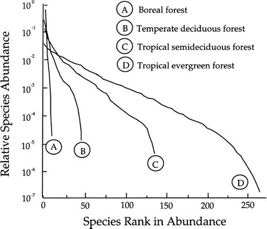
Before delving into this theory and its predictions, it is useful to illustrate briefly the empirical patterns of metacommunity relative species abundance for which we seek a theory. In the first figure of this book (fig. 1.1), I illustrated the dominance-diversity curves for a rather heterogeneous array of communities. However, here I show a more homogeneous set of communities—the relative abundance of tree species in closed-canopy forests—for historical and peda-gogical reasons. I choose them because they are the communities with which I am most familiar and because their dominance-diversity curves are the very ones that stimulated the central theoretical idea in this book. Four dominance-diversity curves for tree communities spanning a latitudinal gradient are shown in figure 5.1. They range from a boreal coniferous forest to a lowland evergreen forest in the equatorial Amazon region.
FIG. 5.1. Dominance-diversity curves for tree species in four closed-canopy forests, spanning a large latitudinal gradient. The four curves seem to represent a single family of mathematical functions, suggesting that a simple theory with few parameters might capture the essential metacommunity patterns of relative species abundance in closed-canopy forests. Redrawn from Hubbell (1979).
The boreal forest is a 0.2 ha sample of the red spruce–Fraser fir community located on the summit of Clingman’s Dome in Great Smoky Mountains National Park (sampled before the advent of acid rain) (Hubbell, unpublished data). This forest displays the geometric progression of relative species abundance characteristic of simple tree communities having high dominance and few (<10) species. This forest is similar to communities that Motomura (1932) described and modeled, and whose relative abundance patterns were later attributed to niche-preemption by Whittaker (1965) (chapter 2). Next there is a distribution for a species-rich, low-elevation temperate forest, a 1 ha sample of cove forest, also in Great Smoky Mountains National Park (Hubbell, unpublished data). This sample has about forty species and exhibits a typical S-shaped lognormal-like distribution of the sort found by Preston (1948). Finally, there are two tropical forests, one relatively species-poor (about 120 species in 13 ha of semideciduous forest in Guanacaste, Costa Rica) (Hubbell 1979), and the other a 4 ha sample of a species-rich (>200 species) evergreen forest near Belém, Brazil) (Hubbell 1979). Both of these tropical tree communities, although represented by different sample sizes, exhibit lognormal-like distributions of relative species abundance. The differences in these dominance-diversity curves are real; they do not result from the different plot sizes.
What is especially intriguing about these dominance-diversity curves is not their differences, but their similarities. The four curves appear to form a single family of closely related functions. This strongly hints that a simple dynamical theory with a parsimonious number of parameters might exist that predicts them all and shows how they are mathematically related. Three of the curves are S-shaped and appear lognormal-like but with different means, variances, and numbers of species. As species richness decreases, the distribution of relative species abundance becomes steeper, and the common species become even more dominant. Thus, there is an increase in the variance of relative species abundance as communities become poorer in species.
The only dominance-diversity curve that would appear not to be lognormal-like is the distribution for the boreal forest. But perhaps this interpretation is incorrect. The smooth progression of the dominance-diversity curves suggests that the boreal forest distribution is just an extreme case of a single process that produces lognormal-like distributions when there are many species, but geometric-like distributions when there are few species. With few species and an especially high variance in relative abundance, the distribution will appear relatively straightened and compressed on a semilog dominance-diversity plot compared to curves for species-rich communities.
Although each of the forests in figure 5.1 is a local community, the patterns in dominance and diversity are qualitatively representative of diversity patterns in boreal, temperate, and tropical forests, and of broad latitudinal changes in metacommunity relative abundance patterns. In island biogeography theory, local community dominance-diversity patterns are expected to be derivative of the metacommunity patterns. Therefore, I first consider the question of the origin and maintenance of species richness, dominance, and diversity in metacommunities. As I will now show, a pattern of dominance-diversity like that in figure 5.1 arises as a consequence of metacommunity dynamics under zero-sum ecological drift. This is the second of the theorems that follow from the biotic saturation of ecological communities (chapter 3).
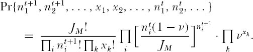
Let us now turn to the problem of the simultaneous zero-sum ecological drift of all the species in the metacommunity. This problem is harder than the one we considered in chapter 4, where we only had to keep track of the dynamics of a single species at a time. An analogous multinomial problem exists in the neutral theory of population genetics, enabling us to take advantage of an analytical strategy developed by Ewens (1972) and Karlin and McGregor (1972) to solve for the metacommunity steady-state dominance-diversity distribution. Let JM be the size of the metacommunity and let ν be the speciation rate. Now consider a discrete-time, nonoverlapping-generations model of metacommunity dynamics. We will assume that the metacommunity is so large that sampling with replacement is a good approximation (cf. chapter 4) so that multinomial probabilities accurately describe processes of ecological drift in the metacommunity undergoing zero-sum dynamics. For simplicity, let a single individual be capable of reproduction. Let  be the abundance of species i in generation t. Then, under ecological drift, the multinomial probability that the abundance of the ith previously extant species will be
  in generation t + 1, i = 1, 2, 3, . . . , plus abundance xk of the kth newly arisen species, k = 1, 2, 3, . . . , is
This multinomial probability implies that, in principle, a specifiable Markovian process exists for the multinomial zero-sum random walk. However, the process is obviously extremely complex, and there are a very large number of states to consider for reasonably large  . Therefore, an alternative analytical strategy is needed to find the stationary dominance-diversity distribution in the metacommunity.
The strategy consists of calculating the unconditional probability as t → ∞ of every possible configuration of relative species abundance in a sample of J individuals drawn at random from the metacommunity. These configurations range from the low-diversity extreme of a single species having J individuals, to the high-diversity extreme of J separate species, each represented by a single individual—and all possible configurations in between. At equilibrium, by definition there is no change in the expected abundances of unlabeled species represented by 1, 2, 3, . . . individuals from one generation to the next. We can make use of this fact to solve the problem. Although the number of probabilities to calculate is still large to very large, it turns out to be possible to write down a fast sampling algorithm for the computation of the equilibrium dominance-diversity curve, the recipe for which is given in chapter 9.
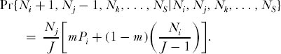
Let us first write down a function for the probability that two individuals drawn at random from the metacommunity in generation t + 1 are of the same species, as a function of the same probability in generation t. If the two individuals are to be of the same species, neither individual can have just speciated, the probability of which is (1 − ν)2. Both individuals can either have had the same parent (with probability 1/) in the preceding generation, or they could have been offspring of different parents of the same species, which in turn shared a common ancestor in some earlier generation. Let  be the probability of drawing two individuals of the same species in generation t+1. Since all individuals of a given species can trace their ancestry back to a common ancestor (the original speciation event), we can write the following recursive function:
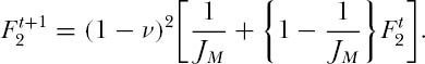
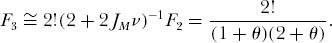
When the metacommunity dominance-diversity equilibrium is reached, then there will be no change in this probability from one generation to the next, i.e.,  . Solving for F2, and ignoring small and higher-order terms in ν, which we can safely do since the speciation rate ν is a very small number relative to unity (e.g., ν
  10−10) we have
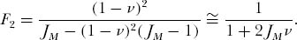
It turns out that 2JMν is a composite parameter that appears throughout the subsequent theory. Because of its fundamental importance, we will give this parameter a special symbol, θ. Thus, θ = 2JMν, and 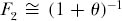 . Although JM is a very large number, and ν is a very small number, the product θ is finite and of intermediate value.
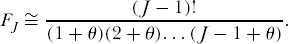
Now consider the probability of drawing three individuals of the same species at random from the metacommunity. None of the three can be a new species [probability (1 − ν)3]. Furthermore, there are now more combinatorial ways of drawing the three individuals of the same species than in the case of two individuals. All three could be offspring of the same parent in generation t, an event with probability (1/JM)2. Or they can have descended from two parents, with probability 3(JM − 1)(1/JM)2. Finally, they could have descended from three different parents of the same species, with probability (JM − 1) (JM − 2) (1/JM)2. This gives the recursive equation
Again, at equilibrium there is no change in this probability between generations t and t + 1, so that  Substituting in the expression for F2 and solving for F3, and again ignoring small and higher-order terms in ν, we obtain
again where θ = 2JMν. By induction, one finds that the probability of drawing J individuals all of the same species is very close to
But this is also the probability that a random sample of J individuals contains just one species. We now need to compute the probability of each multispecies configuration among the J individuals in the sample. So, for example, we can now use FJ to find the probability that a random sample of J individuals contains J − 1 individuals of one species, and one individual of a second species. For any single ordering of individuals, the probability is FJ−1 − FJ. But in this instance there are J possible orderings of {J − 1, 1} individuals in the sample, so the probability is therefore
 for J ≥ 3; and for J = 2, the probability is Pr{1, 1} = θ/(1 + θ).
Continuing in this manner for other multispecies configurations, we can obtain by induction (Karlin and McGregor 1972) the desired unconditional probability for an arbitrary dominance-diversity configuration. For a sample of size J individuals, the probability of obtaining S species with n1, n2, . . . , nS individuals, respectively, where J = ∑ ni, is
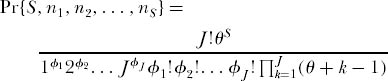
where θ = 2JMν and φi is the number of species that have i individuals in the sample of size J. This proves that under ecological drift there is a nontrivial dominance-diversity equilibrium between speciation and extinction among the unlabeled species in the metacommunity.
However, we are still one step away from having the expected equilibrium dominance-diversity distribution. With no loss in generality, rank order the species in each dominance-diversity configuration, whose probability, Pr{S, n1, n2, . . . , nS}, we have just computed, from the commonest (first position) to the rarest (last position). Let a given ranked dominance-diversity configuration be denoted by {r1, r2, . . . , rS, 0, 0, . . . , 0}, where sufficient zeros are added to fill out the set {ri} to a total of J elements. (The set is filled out to J, because this is the maximum number of species that can occur in a sample of size J.) Adding zeros to the set does not change the corresponding probability, Pr{S, r1, r2, . . . , rS, 0, 0, . . . , 0}.
It is now possible to write down the expected abundance ri of the ith ranked species in the equilibrium metacommunity dominance-diversity distribution for a sample of size J, as follows:
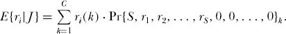
where C is the total number of configurations, ri(k) is the abundance of the ith ranked species in the kth configuration, and Pr{S, r1, r2, . . . , rS, 0, 0, . . . , 0}k is the probability of the kth configuration. The rank order distribution of species abundances, i.e., the metacommunity dominance-diversity curve, is now simply the ordered expectations, E{ri} i = 1, 2, . . . , ordered such that species of the lowest rank are the commonest.
From these results we can compute the expected species richness and relative species abundance in a metacommunity obeying zero-sum ecological drift at equilibrium between speciation and extinction. The preceding two equations are functions of a single parameter θ (apart from sample size J). Since these equations completely determine the metacommunity diversity equilibrium, we have a truly remarkable result: θ controls not only the equilibrium species richness but also the equilibrium relative species abundance in the metacommunity. Parameter θ is a dimensionless, fundamental quantity that appears pervasively throughout the remainder of the theory at all spatio-temporal scales. For this reason, I believe that θ is justifiably named the fundamental biodiversity number.
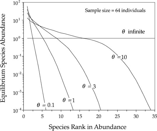
How θ controls the shape of the dominance-diversity curve in the metacommunity is shown in figure 5.2. When θ is small (e.g., 0.1), the expected dominance-diversity curve is steep and geometric-like, with high dominance. However, as θ becomes larger, the expected dominance-diversity distribution becomes more lognormal-like, exhibiting the typical S-shaped curve observed in many species-rich communities (e.g., figure 5.1). At infinite diversity, in the limit as θ → ∞, every individual sampled represents a new and different species, regardless of how large a sample is taken. In this limiting case, the dominance-diversity curve becomes a perfectly horizontal line. At the other extreme, when θ = 0, the distribution collapses to a single monodominant species throughout the metacommunity.
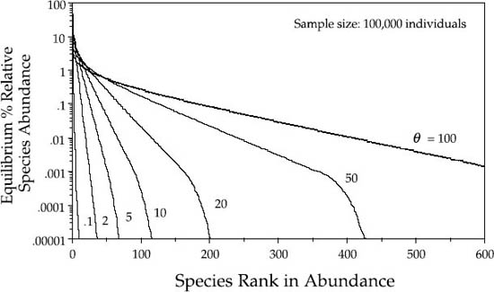
As the sample size increases toward infinity, the expected dominance-diversity curve rapidly converges on a stable relative species abundance distribution for a given θ. The distributions for a sample size of 100,000 are close to the limiting distributions, and are shown in figure 5.3, in which the equilibrium relative abundances are plotted as percentages.
Anticipating a result of chapter 6, it turns out that the fundamental biodiversity number θ is asymptotically identical to Fisher’s α—the measure of diversity in the logseries distribution of Fisher et al. (1943) originally proposed more than 50 years ago. Moreover, the zero-sum multinomial distribution of relative species abundance in the metacommunity is asymptotically identical (in the infinite size limit) to the logseries! Watterson (1976) obtained a similar result for the equivalent genetical theory of Ewens (1972) and Karlin and McGregor (1972). Thus, we finally have a dynamical theory for diversity based on fundamental birth and death processes that justifies the empirically fit logseries distribution of Fisher et al. (1943).
FIG. 5.2. Expected metacommunity dominance-diversity distributions for a sample of 64 individuals, for various values of the parameter, θ. When θ is small, the expected dominance-diversity curve is geometric-like. As θ becomes larger, the expected dominance-diversity curve becomes lognormal-like. As θ → ∞, the distribution approaches a horizontal line. In the limit, when θ is infinite, every individual in the sample is a new and different species, however large a sample is taken.
Recall, however, that Preston (1948) rejected the logseries because it always predicted that there would be more rare species than he observed in his samples of relative species abundance (see chapter 2). When Preston plotted the frequency of species in doubling classes of abundance, in large samples there was almost always an interior mode in one of the abundance octaves representing species having more than a single individual. It was this interior mode which generated the characteristic lognormal-like appearance of the distribution. In contrast, when Fisher’s logseries was similarly plotted, the category of singleton species always had the most species. Preston had no theoretical explanation for his empirical generalization.
FIG. 5.3. As sample size J → ∞, the distribution of relative species abundance approaches a stable limiting distribution of relative abundances for a given value of θ, which is estimated here from a sample of 100,000 individuals.
It turns out that Fisher and Preston were both correct but on very different spatial and temporal scales. According to the unified theory, an interior mode and a lognormal-like distribution (i.e., a zero-sum multinomial) of relative species abundance is expected in a local community or island, whereas a logseries-like distribution is expected in the metacommunity. This is the theoretical expectation only under the point mutation model of speciation, however. Under random fission speciation, the metacommunity distribution is also a zero-sum multinomial, as we shall discover in chapter 8. But for the moment, let us explore why the theory predicts zero-sum multinomial distributions for local communities but logseries-like distributions for the metacommunity under point-mutation speciation. This requires that we now formally unify the theory of biogeography and relative species abundance over the two spatio-temporal scales.
To unify the theory, let us derive the dominance-diversity distribution that arises on an island experiencing immigration from the metacommunity—the classical island-mainland problem posed by MacArthur and Wilson (1967), extended to relative species abundance. Since we have already derived the rank-order abundance distribution for species in the metacommunity, then for the ith ranked species in the metacommunity, we have

From this we see that it is no longer necessary to specify Pi because E{ri} is completely determined by the fundamental biodiversity number, θ. Hence, we can dispense entirely with any and all species-specific parameters in the theory. The unified theory then simplifies to just three parameters: the fundamental biodiversity number θ, the probability of immigration m, and the local community size J. The parameter θ is of course a compound parameter of the metacommunity size JM and the speciation rate ν, but these two parameters appear combined in θ in the theory for point mutation speciation. However, under random fission speciation, it will be necessary to keep these two parameters separate, and then four parameters need to be specified to uniquely determine the metacommunity (chapter 8). To calculate the probability density function for the ith species in the local community, we simply substitute E{ri}/JM for Pi in the eigenvector of equilibrium abundances derived in chapter 4.
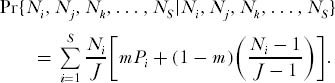
By itself, the eigenvector for the ith species is not sufficient to obtain the multispecies dominance-diversity curve for the local community or island. This requires calculating the equilibrium of the joint random walk, under zero-sum ecological drift, of all species in the local community, and coupled by immigration to the metacommunity. Consider a local community of size J < JM, which is semi-isolated by dispersal limitation from the metacommunity (m < 1). Suppose that there are S species as determined by θ in the metacommunity of size JM. Create a transition probability matrix whose states are all possible combinations of integer abundances of the S species that sum to the local community size J. Consider the analytically more tractable case in which only a single death and replacement occurs (D = 1). In this case, transition probabilities are nonzero only between abundance states that differ by one substitution, or states that remain unchanged. Thus, the probability that species i increases by one individual and species j decreases by one individual is given simply by
and the probability of no change in relative species abundance is
The eigenvector of the matrix of these transition probabilities gives the equilibrium probabilities of each relative abundance combination for the local community distribution. Let this eigenvector be denoted by φ(κ), where κ is the index for each relative abundance combination. Then in strictly analogous fashion to the computation of the dominance-diversity distribution for the metacommunity, the expected abundance of the ranked species in the local community of size J is given by
where C is the total number of configurations, ri(κ) is the abundance of the ith ranked species in the κth configuration, and φ(κ) is the probability of the κth configuration. As in the metacommunity case, the abundances of ranked species, i.e., the local community dominance-diversity curve, is now simply the ordered expectations, E{ri}, i = 1, 2, . . . , ordered such that species of the lowest rank are the commonest. It is important to note in the local community case, unlike the metacommunity, that ri in the above equation does not refer to the rank of the labeled ith species in the metacommunity equilibrium distribution. It refers instead to the ith rank position in the local community, which can be occupied at any given moment by any of the metacommunity species. Thus, the preceding equation computes the expected abundance of the rank 1, 2, 3, et seq. positions regardless of which species currently occupies that rank in the local community. This will be made clearer by following a worked numerical example that is given in chapter 9 for illustration.
The computation of φ(κ) and of the preceding equation is unfortunately only feasible analytically up to a J of about 10, after which the number of combinations of relative abundance makes the analytical approach impractical. Fortunately, the equilibrium distribution of relative species abundance in the local community can be found very simply by simulation even for J values many orders of magnitude larger. The local community distributions of relative species abundance in the remaining part of this chapter are simulation results, but they have all been checked against the analytical results for small JM and J.
This completes the unification of the theory on the local and metacommunity scales and completely solves the classical island-mainland problem of MacArthur and Wilson. We explore the implications of this unification next.
The neutral theory combining the metacommunity and local community dynamics into a single unified theory predicts a new statistical distribution of relative species abundance, the zero-sum multinomial, already alluded to in chapter 3. This distribution describes the relative abundance of species in the local community at dispersal equilibrium with the metacommunity. This distribution is sufficiently close to the lognormal to be easily confused with it, at least in its shape for common species. However, it differs from the lognormal in usually having a long tail of very rare species. An example of a zero-sum multinomial, plotted as a Preston-type curve, is shown in figure 5.4. The zero-sum multinomial is also much more flexible in shape, and its shape is a function not only of the fundamental biodiversity number θ, but also of local community size J and the immigration rate m. Unfortunately, no analytical moment generating function for the zero-sum multinomial distribution is yet available, but the distribution is easily obtained by simulation recipes outlined in chapter 9.
FIG. 5.4. An example of a zero-sum multinomial distribution, showing its typical skewing with a long tail of very rare species. This is the distribution predicted by the unified neutral theory for the distribution of relative species abundance in a local community at an immigration-extinction steady state with the metacommunity source area.
We can also examine the shape of the zero-sum multinomial as a Whittaker-style dominance-diversity curve. When the immigration rate is greater than zero, a nontrivial equilibrium dominance-diversity distribution arises in the local community or island as a steady state between immigration and local extinction—just as MacArthur and Wilson’s theory predicted a nontrivial island equilibrium in species richness. Consider a model island community of size J = 1600 experiencing different immigration rates from the metacommunity source area. We obtain a family of equilibrium island dominance-diversity distributions whose shapes depend upon the immigration rate (fig. 5.5).
When all of the deaths due to disturbance are replaced by immigrants, the dominance-diversity curve is the same as that of the metacommunity (i.e., logseries-like), with identical relative abundances as expected for a sample of size J individuals from the metacommunity. However, as fewer local deaths are replaced by immigrant individuals, the equilibrium dominance-diversity curve for the local community becomes steeper and more geometric-like. Note that it takes rather severe isolation to produce extremely steep dominance-diversity distributions—unless the metacommunity itself is species poor. For example, the steepest of the curves in figure 5.5 corresponds to just a single immigrant per 10,000 deaths. Conversely, when only 10% of the deaths are replaced by immigrants, the equilibrium dominance-diversity curve is still very similar to the source area distribution. All of these local distributions are examples of the zero-sum multinomial distribution. Thus, the unified theory predicts that the local community distribution of relative species abundances will differentiate in both shape and in total species richness from the mainland metacommunity distribution. We can now state a general principle: on islands, common species will be commoner, and rare species rarer, than in the metacommunity. The degree of this differentiation is determined by the degree of isolation of the local community from the mainland, which in turn is controlled by the immigration rate m.
FIG. 5.5. Equilibrium island dominance-diversity distributions for an island under different rates of immigration from a mainland source area. Island community size has been set at 1600 individuals in this numerical example. The bold line is the expected dominance-diversity distribution if all deaths are replaced by immigrants from the source area. The equilibrium distribution becomes steeper and more geometric-like with increasing isolation from the metacommunity.
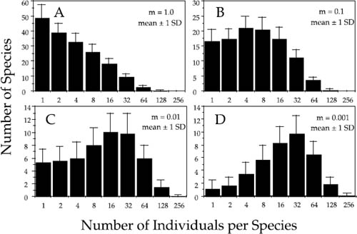
Herein lies the explanation for why Fisher and Preston were both correct. If we replot the relative species abundance distributions for the local community as Preston-type frequency plots, it is clear why (fig. 5.6). Consider once again a local community of size J = 1600. At infinite dispersal (m = 1), the local community is not isolated from the metacommunity. In this limiting case, the local relative abundance distribution will be a random sample of the metacommunity logseries-like distribution, and singleton species will be the most frequent abundance class in a Preston-type plot (panel A). However, as m becomes smaller, the island or local community becomes progressively more isolated, and the shape of the relative abundance distribution changes (panels B–D). As m decreases, rare species become rarer and less often present, and common species become commoner and more consistently present, in the local community. This results in a depression of the abundances of rare species and a rightward shift of the mode of the distribution to higher-abundance classes.
FIG. 5.6. The effect of dispersal limitation (isolation) on the expected zero-sum multinomial distribution of relative species abundance in a model local community or island according to the unified neutral theory. Relative abundance distributions are plotted by doubling classes of abundance, following the method of Preston (1948). In all panels, the error bars represent ±1 standard deviation. (A) – (D): Model community of J = 1600 individuals and θ = 50. (A) No dispersal limitation (m = 1). This is the distribution of relative species abundance expected in a random sample of 1600 individuals from the metacommunity logseries. (B) Relatively low local community isolation and dispersal limitation (m = 0.1). (C) Moderate isolation and dispersal limitation (m = 0.01). (D) Severe isolation and dispersal limitation (m = 0.001).
The unified theory thus predicts that the shape of the local distribution of relative species abundance will be a function of the immigration rate. This is the resolution of the conflict between Fisher and Preston. The unified theory explains the interior mode of the relative abundance distribution discovered by Preston as simply the result of restricted immigration, i.e., dispersal limitation. Thus, Preston’s distribution was a sampling theory for relative species abundance in local communities, whereas Fisher’s distribution, as we now realize in retrospect, was a sampling theory for the metacommunity.
These changes in shape also explain the asymmetry observed in the local distribution of relative species abundance in many Preston plots of empirical data. Recall from chapter 3, for example, that the Preston plots of relative species abundance in the 50 ha permanent plots in Pasoh Forest Reserve, Peninsular Malaysia, and on Barro Colorado Island (BCI), Panama, showed large excesses of rare species over what was predicted by the best-fit lognormal (see figs. 3.3, 3.4).
I have replotted the BCI and Pasoh distributions in figures 5.7 and 5.8, respectively, showing that the zero-sum multinomial distribution of the unified neutral theory fits the empirical distributions much better than the lognormal. The neutral theory achieves this improved fit with no more parameters than the lognormal (three). Probably more important than the number of parameters, however, is the fact that, for the first time, the parameters of the distribution are interpretable in terms of a birth-death-dispersal process. They aren’t simply fitted means and variances of a generic statistical distribution. Moreover, because the theory generating the relative abundance distribution is dynamical, for the first time we can also put error bars on the expected number of species in each abundance class. These error bars arise from the demographic and community stochasticity underlying zero-sum ecological drift, and they are calculated from the expected variances in the steady-state relative abundance distribution.
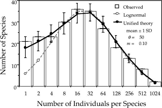
FIG. 5.7. Preston-type plot of relative species abundance for tree species >10 cm dbh in the 50 ha BCI plot, compared with expectations from the lognormal, and from the zero-sum multinomial of the unified neutral theory, for θ = 50 and m = 0.10. The error bars are ±1 standard deviation.
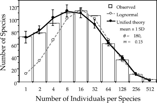
FIG. 5.8. Preston-type plot of relative species abundance for tree species >10 cm dbh in the 50 ha Pasoh plot, compared with expectations from the lognormal, and from the zero-sum multinomial of the unified neutral theory, for θ = 180 and m = 0.15. The error bars are ±1 standard deviation.
Because the relative abundance distribution is a function of the immigration rate, we can use changes in shape of the distribution to estimate parameter m and thereby quantify the average dispersal limitation and degree of isolation affecting a given local community or island. For example, the estimated value of m for the BCI plot is 0.10. This is equivalent to the statement that 90% of the trees in the plot have been locally produced (“births”), and 10% were immigrants. This is a reasonable value for m given that 10% of the area of the plot lies within 17 m of the outer perimeter. The estimate of m for the Pasoh plot is slightly higher: 0.15. The main canopy at Pasoh is twice as high as at BCI (50 m vs. 25 m), which may mean that seeds disperse slightly farther in absolute distance from the average tree crown in the Pasoh forest. Once dispersal limitation is factored in, the expected equilibrium relative abundance distributions fit the observed distributions almost exactly (figs. 5.7, 5.8).
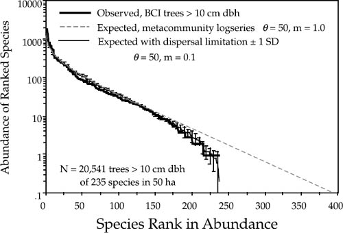
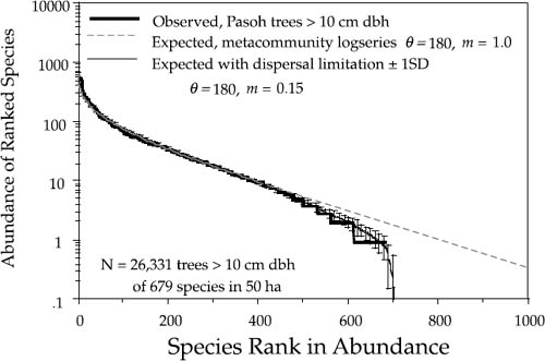
The goodness of fit of the theoretical distributions to observed dominance-diversity curves is often quite remarkable. This is a much more demanding fitting exercise than the Preston-type plot because the abundances of all species are individually displayed and ranked in the curve. I have plotted the dominance-diversity curves for BCI and Pasoh in figures 5.9 and 5.10, respectively.
The expected metacommunity logseries relative abundance distribution was calculated from a sample size of 1,000,000 (see fig. 5.3). It was then scaled to local community size for comparison to the local distribution in each figure. The metacommunity logseries distribution is the diagonal line extending downward beyond the empirical curves to the lower right. The metacommunity distribution was calculated for a fitted θ value of 50 in the case of the BCI forest, and for a fitted θ value of 180 in the Pasoh forest. Then the parameters for dispersal limitation and local community size were included to predict the local community dominance-diversity curves in each forest plot. Local community size was 20,541 trees > 10 cm dbh in the BCI plot, but it was 28% higher (26,331) in the Pasoh plot. The previously estimated values of m of 0.10 and 0.15 for BCI and Pasoh, respectively, were used. The precision of the predicted local dominance-diversity curves in each plot is readily apparent from figures 5.9 and 5.10. The expected distributions fit even the abundances of the rarest species extremely well. The process of parameter estimation under the unified theory is discussed in detail in chapter 9.
FIG. 5.9. Fitted and observed dominance-diversity distributions for trees >10 cm dbh in the 50 ha plot on Barro Colorado Island, Panama. The best fit θ had a value of 50. Note the departure of the metacommunity distribution for very rare species, but that the observed distribution is fit well once dispersal limitation (m = 0.10) is taken into account. The error bars are ±1 standard deviation.
FIG. 5.10. Fitted and observed dominance-diversity distributions for trees > 10 cm dbh in the 50 ha plot in Pasoh Forest Reserve, Malaysia. The best fit θ had a value of 180. Note the departure of the metacommunity distribution for very rare species, but that the observed distribution is fit well once dispersal limitation (m = 0.15) is taken into account. The error bars are ±1 standard deviation.
The unified theory predicts that rare species will be even rarer and less frequent on islands or in local communities than one would expect from their metacommunity relative abundances. The theory explains this phenomenon as an interaction between dispersal limitation and extinction-proneness of rare species on islands. Rare species are more likely to go extinct per unit time, and are less likely to reimmigrate after local extinction, than common metacommunity species. The net result is that at equilibrium, rare species will constitute a smaller fraction of the community on islands than in the mainland metacommunity. This has important implications for conservation, because it means that rare species will be harder to conserve in a fragmented landscape.
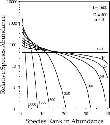
Let us now consider a case that is more like the classical island-mainland case discussed by MacArthur and Wilson. Their theory hypothesized that the lower species richness on oceanic islands compared to same-sized sample areas on the mainland was due in part to lower rates of immigration than would occur among adjacent areas of a continuous mainland (chapter 1). The best test of the theory’s predictions would be a case in which islands were once connected to a mainland but subsequently became isolated from it. If the immigration to an island is suddenly greatly reduced, the island will experience a steady loss in species richness, accompanied by a shift to more geometric-like, dominance-diversity distributions. Figure 5.11 illustrates the transient behavior expected during diversity loss in a model island community of size J = 1600 individuals that is completely isolated from the mainland metacommunity. For illustrative purposes, the initial community on the island was started with forty equally abundant species. In this case of complete isolation, the equilibrium community is a single monodominant species.
FIG. 5.11. Transient dynamics of the dominance-diversity curve in an island community of size J = 1600 undergoing zero-sum ecological drift under complete isolation from the metacommunity. Numbers indicate how many disturbance cycles since the island community was initiated with initiated with forty equally abundant species. The absolute death rate per disturbance is 400 in this example.
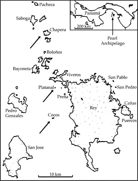
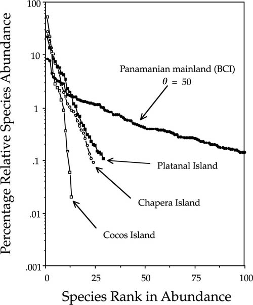
Such a test was possible in the Pearl Archipelago in the Bay of Panama (fig. 5.12). Several years ago, S. J. Wright enumerated tree species >10 cm dbh on three small islands (Chapera, Cocos, and Platanal) with similar topography, soils, and climate in the Pearl Archipelago in the Bay of Panama. During the Wisconsin glacial maximum, these islands were part of a broad, continuous coastal plain attached to the mainland. At that time they presumably had the full complement of mainland tree species. However, since isolation, they would have been expected to lose species through local extinction, and this appears to have been the case (fig. 5.13), as predicted by the theory of island biogeography. If the unified neutral theory applies as well, then the dominance-diversity distributions for the tree communities on these islands should also have become steeper and more geometric-like. This too is observed. The most abundant species reached levels of dominance more typical of a temperate deciduous forest than of a tropical forest. Each island ended up with a different dominant species in spite of similar topography, soils, and climate, also consistent with ecological drift.
The steepness of the dominance-diversity curves, and their nearly geometric form, suggests that these islands now experience low to very low immigration rates of trees. Suppose we can assume that these islands have reached their equilibrium dominance-diversity distributions. Then we can estimate the immigration probabilities for each island, assuming equilibrium, which are on the order of a low of six in 10,000 births for Cocos Island to a high of seven in 1000 births for Platanal Island (Hubbell 1997). Cocos, the smallest and most remote island, had the steepest dominance-diversity curve and the fewest species, as expected. Platanal, the next-smallest island, nevertheless had the greatest species richness and the shallowest dominance-diversity curve. The proximity of Platanal Island to Rey Island, the largest of the islands in the archipelago (fig. 5.12), may explain Platanal’s higher diversity. Chapera, the largest of the three islands but also fairly remote from potential source areas, had intermediate tree species richness and dominance diversity. As predicted by theory, the variance in relative species abundance was greater on the islands than on the mainland. Dominance of the rank-1 species ranged from 29% on Platanal to 52% on Cocos Island.
FIG. 5.12. Map of the Pearl Archipelago of islands off the southern coast of Panama. These islands were connected to the mainland during the Wisconsin glacial maximum, but became isolated about 10,000 years ago, when rising sea levels drowned the Pacific coastal plain. Tree communities were enumerated (trees > 10 cm dbh) on three islands—Chapera, Cocos, and Platanal—by S. J. Wright of the Smithsonian Tropical Research Institute.
FIG. 5.13. The dominance-diversity distributions for the tree communities on Chapera, Cocos, and Platanal Islands of the Pearl Archipelago, compared to the dominance diversity for the forest on Barro Colorado Island (BCI), which serves as a representative Panamanian mainland site. The BCI data are truncated at one hundred species so that the dominance-diversity curves for the islands can be better displayed. Las Perlas data courtesy of S. J. Wright, Smithsonian Tropical Research Institute.
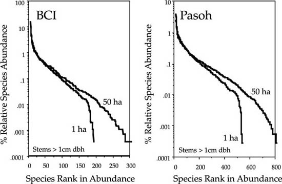
If dispersal limitation in combination with local extinction is causing relative species abundances to differentiate on islands, a similar but weaker effect ought to be detectable in local stands of forest on continuous landscapes. In both the BCI and Pasoh plots we can, in fact, detect the predicted small shift in the shape of the dominance-diversity distributions in single hectares of forest relative to the 50 ha plot as a whole (fig. 5.14). These curves are compared on a percentage dominance basis to normalize the distributions for different total numbers of trees in 1 vs. 50 ha. As predicted, there is both a slight increase in dominance and a steepening of the dominance-diversity distribution in 1 ha plots vs. the entire 50 ha plot in both forests. In spite of major differences in species composition, stem density, tree species richness, and fitted θ values, the BCI and Pasoh forests are remarkably similar in the small-scale spatial differentiation of their dominance-diversity curves. The tailing-off of the rare species in the plots is as predicted from the greater effect of dispersal limitation on rare species.
FIG. 5.14. Small-scale spatial differentiation of the dominance-diversity curve within the 50 ha plots on Barro Colorado Island, Panama (left), and in Pasoh Forest Reserve, Malaysia (right). The mean dominance-diversity curve for single hectares is shown along with the curve for the entire respective 50 ha plot.
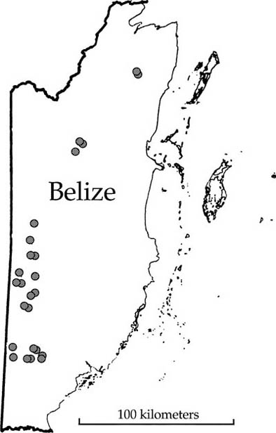
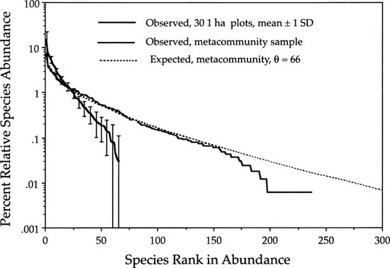
We also find a similar differentiation of local and regional dominance-diversity curves on much larger spatial scales. For example, here are data from a study of the forests of Belize (Bird 1998). A series of 1 ha plots was established in closed-canopy forest in a 200 km north-south transect running most of the length of the country (fig. 5.15). We can use the total dataset as a measure of metacommunity biodiversity, and compare this with the biodiversity of the 1 ha plots. When we do this, we obtain a very good fit for the metacommunity with a θ of 66 (fig. 5.16). There is a slight tailing-off of rare species even in this dataset, indicating that there is dispersal limitation even at these very large geographical scales. However, there is much stronger evidence of dispersal limitation for the 1 ha plots, which show much greater dominance, fewer species, and steeper dominance-diversity curves, as predicted. The abundance of the rank-1 species in the 1 ha plots is about 15%, but it is only about 6% in the entire metacommunity.
FIG. 5.15. Map of Belize showing the locations of thirty-eight 1 ha plots of closed-canopy forest in a 200 km north-south transect. Data from Bird (1998).
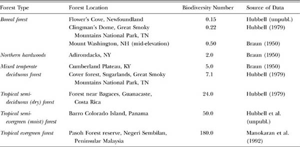
Before concluding this chapter, it is worth taking a closer look at the fundamental biodiversity number θ. The paramount importance of θ is that, for the first time, we have a formal theory of biogeography that ties speciation to patterns of diversity and relative species abundance on local to regional scales. Earlier I described latitudinal gradients in dominance-diversity patterns in closed-canopy forests (fig. 5.1). When θ is fitted to a geographical range of tree communities, values vary from a low of 0.15 for a sample of boreal spruce-fir forest in northern Newfoundland, to a high of 180 for Pasoh, a tropical lowland mixed-dipterocarp evergreen forest in Malaysia (table 5.1). The neutral theory explains these broad latitudinal patterns of dominance diversity in tree metacommunities as primarily the result of geographical variation in the fundamental biodiversity number θ.
FIG. 5.16. The dominance-diversity curves for the forest of Belize. The pooled dataset for all thirty-eight 1 ha plots is quite well fit by a θ of 66. Nevertheless, even the metacommunity shows some evidence of dispersal limitation in the tailing off of the abundances of very rare species. The observed mean and standard deviations of the 1 ha plots show much greater dispersal limitation, and species richness is less than a third of the regional species richness. Data obtained from Bird (1998).
Why is there geographic variation in θ? It could arise through systematic geographic variation in the size of metacommunities, in the speciation rate, or in some combination of the two. The metacommunity dominance-diversity equilibrium will also reflect variation in exogenous extinction rates that are additional to those expected under ecological drift. In high-latitude forests, speciation rates appear to be low relative to extinction rates, and geometric-like distributions obtain. Conversely, at equatorial latitudes, speciation rates are evidently high relative to extinction rates, and so species accumulate, resulting in very flat, lognormal-like steady-state distributions of relative species abundance. As I will discuss further in chapter 6, dispersal limitation also increases steady-state metacommunity diversity. The theory does not explain why extinction rates should be higher relative to speciation rates at high latitudes. One possibility is that disturbances are more frequent and/or more severe in high-latitude communities, elevating extinction rates relative to speciation rates. This was the thesis of the time-stability hypothesis put forward by Sanders (1968, 1969) and Slobodkin and Sanders (1969). They argued that the relatively greater age and stability of the tropics has allowed species to accumulate in the tropics and persist longer before extinction occurs. Another contributing factor is undoubtedly a simple climate-area effect. Terborgh (1973) has noted that there is far more land area per degree temperature change in the tropics than there is at higher latitudes.
TABLE 5.1. Estimated values of the fundamental biodiversity number θ for a broad range of closed-canopy tree communities, mainly New World
I do not know how large realized θ values can become, but probably very large in microbial communities. Recent work inferring the diversity of soil microbial communities from surveys of DNA sequence variation for both culturable and nonculturable species suggests that, while diversity is not infinite, it is very large. John Tiedje (pers. comm.) found no repeats in more than four hundered strain isolates, i.e., a perfectly flat dominance diversity curve with every “species” represented by one and only one sample.
The fundamental diversity number θ is remarkable because it is finite and a moderately sized number. Its finiteness is remarkable because θ is the product of two numbers that differ enormously in size: the metacommunity size, JM, and the speciation rate, ν (times two). We know very little about these numbers, but we can be certain that the speciation rate per birth is a very small number. Because the observed value of θ ranges roughly between 0.1 and 200, we must conclude that the metacommunity size JM must be a very large number, i.e., on the order of 0.05 to 100 times the inverse of the speciation rate. For example, suppose the speciation rate is one in a trillion (1012) births. Then the metacommunity size must be between roughly 50 billion (5 · 1010) and 10 trillion (1014) individuals (births).
What is a reasonable size for the speciation rate or for the metacommunity? At this point it is difficult to say. The value of θ can be held constant if the size of the metacommunity is reduced but the speciation rate is increased to compensate. I will return to the question of estimating speciation rates in chapter 8 and discuss the implied magnitude of speciation rates in greater detail then.
Because of the difficulty of coping with such large numbers of individuals, it may be easier to use an area-based formula for θ rather than an individual-based formula. Note that θ can also be written as a simple linear function of the area AM occupied by the metacommunity:
θ = 2ρAMν,
where ρ is the mean density of individuals per unit area in the metacommunity. Note that this formula shows that the fundamental biodiversity number θ is directly tied to the biotic saturation of landscapes. Note also that ρ measures the productivity of a unit of area in landscapes to support organisms. Therefore, θ ties the biodiversity of the metacommunity directly to the productivity of the landscape.
The unified neutral theory thus reaches the simple but potentially profound conclusion that one can predict both the species richness and relative species abundance in a metacommunity undergoing zero-sum ecological drift by knowing just a few things. One needs to know the area and the average speciation rate in the biogeographic region, the density of organisms per unit area, and, finally (as I shall show in chapter 6), the mean dispersal rate of species over the landscape. With these few parameters, the neutral theory gives a complete description of the metacommunity under ecological drift, random dispersal, and random speciation. The unified theory appears capable of explaining many broad as well as specific patterns in relative species abundance in ecological communities from a few very simple neutral assumptions. The generality of the theory as applied to a wide variety of communities will be explored more fully in chapters 9 and 10.
One of the most important findings of the unified theory is that metacommunity dynamics are so slow under drift that ecological and evolutionary rates of change will become commensurate on large landscape scales. Indeed, this must be true because we can prove that a diversity equilibrium will inevitably arise between speciation and extinction in the metacommunity. It is largely this single fact that has made a unified theory of biogeography, speciation, and relative species abundance a reasonable goal to pursue.
1. The unified neutral theory predicts the existence of a dimensionless biodiversity number θ, which is equal to twice the speciation rate times the metacommunity size. This number appears to be fundamental in the sense that it appears throughout the theory at all spatio-temporal scales.
2. Under the “point mutation” mode of speciation, a formula containing θ as the only parameter completely controls metacommunity species richness and relative species abundance at steady state between speciation and extinction.
3. With two additional parameters, immigration rate and local community (island) size, the neutral theory also predicts species richness and relative species abundance in local communities (islands).
4. This relative abundance distribution on islands (local communities) is a new statistical distribution called a zero-sum multinomial, whose shape depends on θ, the size of the local community (island), and the immigration rate. The distribution usually has a long tail of very rare species. It can be logseries-like, lognormal-like, or geometric-like, depending on the degree of isolation from the metacommunity source area.
5. On islands (local communities), common species are commoner and rare species are rarer and less numerous than expected from random samples of the metacommunity. This is because rare species are more extinction prone and less likely to reimmigrate quickly after local extinction.
6. These results reconcile the classical dispute between Preston and Fisher over the shape of the relative abundance distribution. In retrospect it is clear that Fisher was describing the metacommunity sampling distribution, whereas Preston was describing the local community distribution.