I have deferred until now issues of sampling and parameter estimation in the unified theory, as well as a discussion of the theory’s generality. I first consider sampling, which might seem a prosaic and uninteresting subject. But one of the big questions about biodiversity that has captured considerable attention recently is a sampling question, namely: How many species are there on Earth—or on any part of it (Erwin 1982, May 1988, Wilsm 1995)? Because of the potentially fractal nature of biodiversity, there is an issue of how one identifies and tallies taxonomic units in the unified theory (chapter 8), but for the moment we can set this problem aside. The answer to this question is less important than understanding the biology of species and their interactions in communities (Janzen 1997). However, in attempting to answer it we also learn about the processes underlying the origin, maintenance, and loss of biodiversity. To be meaningful we need to restrict our question to some particular taxon or trophically defined community. For some groups of organisms, particularly large or charismatic taxa such as birds, large mammals, and butterflies, groups which are well known, there is little difficulty in enumerating the species. However, for many groups of invertebrates and microorganisms, this question has proven to be an extraordinarily difficult challenge to ecologists, systematists, and biogeographers (Erwin 1997, Stork 1997, Wheeler and Cracraft 1997).
In any case, asking how many species there are is fundamentally a sampling question. Total counts might seem appealing at first because they appear to have greater objectivity and precision than estimates based on sampling, but this is not necessarily so. Moreover, a total count of the world’s species is not feasible—and not even approachable without heroic international investments of time, human resources, and money. Even the more modest goals of making complete species inventories of particular communities or ecosystems (e.g., “All Taxa Biological Inventories,” Janzen and Hallwachs 1994) have had to face extraordinary difficulties, not the least of which is the global shortage of trained taxonomists (Wheeler and Cracraft 1997). I am not suggesting that we should abandon these efforts. Quite the contrary, systematics provides the critical information base for all of ecology and biogeography, and we need to increase the number of taxonomists. However, these efforts could be considerably strengthened by having a strong sampling strategy based on a sound theory of biodiversity. Such a theory could help answer the question of how many species there are much more rapidly, accurately, and economically.
Both Fisher et al. (1943) and Preston (1948) had sampling theories that could be used to estimate the total number of species as well as relative species abundance. Indeed, that the logseries and lognormal had sampling theories is probably the single most important reason why so much attention has been devoted to fitting these distributions to empirical data (Anscombe 1950, Bliss and Fisher 1953, Patrick et al. 1954, Preston 1962, Williams 1964, Patrick 1968, 1972, Bulmer 1974, Kempton and Taylor 1974, May 1975, Pielou 1975, Taylor et al. 1976, Slocumb et al. 1977, Engen 1978, Gray 1979, 1981, Routledge 1980, Sugihara 1980; see also reviews in Magurran 1988 and Tokeshi 1993, 1997, 1999). However, Fisher and Preston had no underlying theory of population and community dynamics from which to derive expected distributions of relative species abundance. If a distribution fits or fails to fit the data adequately, it is unclear what significance to attach to this result because the parameters of the lognormal and logseries are generic (e.g., mean, variance, Fisher’s α, etc.). These generic parameters do not reveal their derivation from fundamental processes of birth, death, migration, and speciation. This derivation is now clarified by the unified theory.
However, Preston (1948, 1962) concluded erroneously that it was possible to obtain a good estimate of the total number of species in the community from the lognormal (chapter 2). Because the lognormal is a symmetrical distribution, Preston thought that, once sample sizes were large enough to reveal the mode, one could estimate the total number of species in the community simply by doubling the number of species to the right of the mode. But as we have noted in previous chapters, virtually all observed distributions of relative species abundance for large sample sizes are negatively skewed, with a long left-hand tail and a large excess of rare species over what is predicted by the lognormal.
According to the unified neutral theory, the distribution of relative species abundance in local communities is better described by the asymmetric zero-sum multinomial distribution than by the symmetric lognormal. On larger landscapes the theory predicts that the metacommunity distribution will either be the logseries or the zero-sum multinomial, depending on the prevailing mode of speciation. Like Fisher’s and Preston’s theories, the zero-sum multinomial also has an associated sampling theory. Unfortunately, this sampling theory is not analytically tractable except for very small community sizes (see below). As a result, almost always the parameters of the zero-sum multinomial must be estimated by simulation. It is possible that further analytical work will enable discovery of a generating function for the zero-sum multinomial, but currently none exists. In order to make the zero-sum multinomial more user-friendly for the present, we intend to publish tables of the distribution for a very large set of possible parameter values. These will be provided on some medium such as CD-ROM or on the Internet. A fitting routine will also be available in this statistical package for fitting the user’s relative abundance data.
The theory via simulation permits us to estimate the mean and variance of the total number of species in a local community, as well as the expected number of species in a subsample of the community of arbitrary size J. We can also estimate the mean and variance of the total number of species in the entire metacommunity if the size of the metacommunity is known or estimable. The total number of species in the metacommunity will have a sample variance and not be a constant because the steady-state metacommunity biodiversity is a stochastic equilibrium. Sometimes there will be more, and sometimes fewer species, depending on the actual history of random births and deaths.
The total number of species in the metacommunity can, in principle, be estimated from a finite and relatively small random sample of the metacommunity and from the density of individuals and the area occupied by the metacommunity. The estimate of the fundamental biodiversity number θ will be best if the sample truly is random. However, in most real-life situations, ecologists will have a dataset for a particular local community. This community is expected to exhibit differentiated relative abundances that reflect its size and isolation from the metacommunity. If the metacommunity relative abundance distribution is logseries, then, in principle, the fit of θ to the data should yield an estimate of the fundamental biodiversity number. As we have seen in chapter 5, the number θ is asymptotically identical to Fisher’s α, which explains why the number is so stable in the face of increasing sample size. However, if the dispersal limitation affecting the local community is strong, it is likely that the true metacommunity value of θ will be underestimated. An illustration of this fitting problem can be found in the data for tree diversity in Belize forests (fig. 5.16). If all one had were the 68 1-hectare plots, the fitted value of θ would be around 11. However, when we pooled all the data from the entire length of the country, the metacommunity data fit well with a θ of 66. If one knows the value of θ for the metacommunity, then it is possible to estimate the degree of dispersal limitation and the parameter m from the degree of which local relative abundances have differentiated from the metacommunity relative abundance distribution. Because common local species are likely to be widespread metacommunity species, a better estimate can often be obtained from fitting only the common species in the local community. I will have more to say on this below.
A caveat is needed at this point. The fitting of the fundamental biodiversity number θ to relative abundance data is just that. It does not actually “test” the assumptions of the theory behind the number. To do that will require independently estimating the speciation rate ν and the metacommunity size JM. If it is possible to obtain reliable estimates for these two numbers, then an independent calculation of θ will be possible to compare with the fitted values obtained from relative abundance data. However, as we have argued in the last chapter, all of our current estimates of speciation rate are biased low, and it is difficult to say at the present time how serious this bias may be (chapter 8).
So let us now look in more detail at the problem of finding the expected values for the relative abundance distributions predicted by the unified theory. In chapter 5 I proved that, under point mutation speciation and in the implicit spatial case, the metacommunity distribution of relative species abundance at equilibrium between speciation and extinction is completely specified by the parameter θ, a composite of metacommunity size JM and speciation rate ν. However, in chapter 6 I showed that in explicitly spatial models, obtaining the metacommunity distribution then also requires estimating the dispersal rate m.
In principle, the exact expectations are computable for any community size, but in practice only for J up to about 10, which is far too small a community to be biologically interesting. Fortunately, the expected values can be found to an arbitrary degree of accuracy by simulation, even for very large community sizes (e.g., JM or J > 1010). Before discussing the simulation recipe, however, it is important to study the analytical answers for small JM and J. Though tedious to compute, they are important checks to ensure that one’s simulations are indeed generating the right expected values. For this reason, I briefly outline the procedure used in the analytical calculation of expected multispecies relative abundances. The expectations can be found exactly numerically for small JM and J from the multispecies version of the zero-sum random walk of the ith species studied in chapter 4.
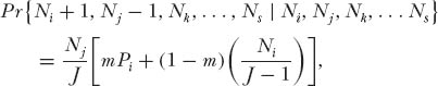
The procedure is a two-step process. The first step is to calculate the logseries expectations of relative species in the metacommunity of size JM with fundamental biodiversity number θ from the expressions derived in chapter 5. The abundances expressed as a fraction of JM are the expected proportional relative species abundances Pi in the metacommunity. The second step is to calculate the relative abundances in the local community. Consider a local community of size J < JM, which is semi-isolated by dispersal limitation from the metacommunity (m < 1). Suppose that there were S species in the metacommunity of size JM. Create a transition probability matrix whose states are all possible combinations of integer abundances of the S species that sum to the local community size J. Consider the case in which only a single death and replacement occurs. In the case of D = 1, transition probabilities are nonzero only between abundance states that differ by one substitution, or states that remain unchanged. Thus, the probability that species i increases by one individual and species j decreases by one individual is given simply by
and the probability of no change in relative species abundance is
As J and S become larger, the number of possible integer combinations of relative abundance rapidly becomes very large. For example, for J = 10, the number of unique combinations of relative abundance (integers adding up to 10) is 42; but the number of corresponding combinations of 10 species for these combinations of relative abundance is 6360. For J = 20, these numbers increase to 627 and 4.67 × 10⁷, respectively! Fortunately, we can reduce the dimensionality of the matrix by combining states for all species combinations that represent the same distribution of relative abundance. But to do so, we must sum all the transition probabilities for all named species for a given relative abundance distribution. A computer program can be written to do this. The necessary program calculates the transition probabilities among the states, which comprise all possible distributions of relative species abundance that sum to J. Now find the eigenvector of this numeric matrix. This eigenvector gives the unconditional (equilibrium) probability of each possible combination of relative species abundance in the local community of size J. Finally, calculate the expected abundance of the ranked species, by taking the abundance of the rth ranked species in each relative abundance distribution (state), and multiply it by the eigenvector probability for that state. Then sum these products for the rth ranked species in all states. The sum thus obtained is the analytically expected relative abundance of the rth ranked species in the local community.
A worked numerical example may make the process clearer. Suppose the metacommunity contains three species A, B, and C, each with the same metacommunity abundance (P = 1/3), and let the immigration probability be relatively modest (m = 0.1). Suppose we let local community size J = 3. There are then ten possible states of relative abundance and species mixtures. The ten states are: three monodominant states: (3A), (3B), and (3C); six states with two species (2A, 1B), (2A, 1C), (2B, 1A), (2B, 1C), (2C, 1A), and (2C, 1B); and one state with all three species (1A, 1B, 1C). Permutations of species order do not matter. These ten species-combination states correspond to just three relative abundance states (3), (2, 1), and (1, 1, 1). The eigenvector for the ten-state matrix is { 0.2723, 0.2723, 0.2723, 0.0292, 0.0292, 0.0292, 0.0292, 0.0292, 0.0292, 0.0079 }, corresponding to the species mixtures in the order listed above. The first three states all have the same equilibrium probability (the monodominant states) as do the middle six states (the two-species combinations) because we chose our metacommunity relative abundances of the three species to be equal. The reduced matrix with three relative abundance states has the eigenvector { 0.8169, 0.1752, 0.0079 }, corresponding to states (3), (2, 1), and (1, 1, 1).
The final step is to calculate the expected relative abundances of the ranked species. In the convention used throughout this book (and in the literature as well), species tied in rank are not given mean rank scores, but are simply assigned the tied cardinal ranks at random. This is the only way that computation of mean abundance of ranked species makes sense. In the present example, the expected abundance of the rank-1 species is 3(0.8169) + 2(0.1752) + 1(0.0079) = 2.8090; the expected abundance of the rank-2 species is 1(0.1752) + 1(0.0079) = 0.1831; and the expected abundance of the rank-3 species is 1(0.0079) = 0.0079. The sum of these expected abundances is 3.0000, which is equal to J, completing the analytical result.
This numerical example is useful for demonstrating that a semi-isolated habitat or island will always differentiate a steeper dominance diversity curve than the dominance diversity curve for the metacommunity or mainland. The effect of isolation on relative species abundance is dramatized especially in this example because all the species in the metacommunity were given equal abundances.
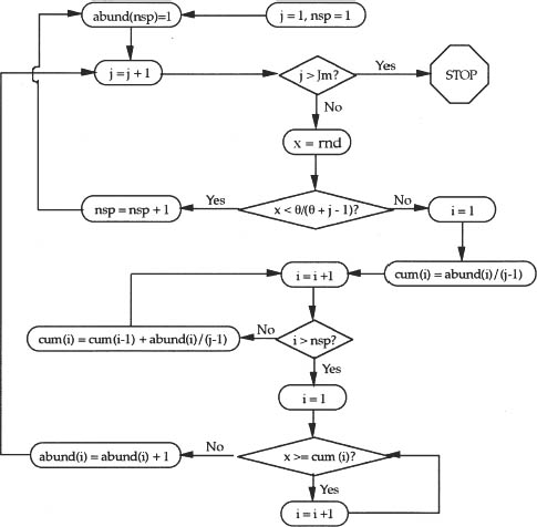
In almost all calculations of expected values, the preceding analytical approach will not be pursued because of the computational problems posed by large JM and J. I now discuss a simulation algorithm which works for large and small J. The following recipe is due to Warren Ewens (pers. comm.). Call the quantity θ/(θ + j − 1) the species generator. It represents the probability that the next individual sampled is of a new species not previously collected. Draw the first individual, and label it species 1. Now collect the second individual, and draw a random uniform number x between zero and one. If x is less than the value of the species generator for J = 2, i.e., x < θ/(θ + 1), then individual 2 is a new species. However, if x > θ/(θ + 1), then the second individual is another specimen of the first species. Now collect the third individual and draw a new random uniform number x between zero and one. If x is less than the species generator for J = 3, i.e., if x < θ/(θ + 2), then the third individual is a new species; otherwise, it belongs to a species previously encountered.
In this case, since the individual is of a previously encountered species, we must determine to which of these already collected species the individual belongs. Do the following. First, calculate the current fractional abundance of each species from the first species to the last species found. Suppose the current abundance of the ith species is ni before adding the jth individual. Then the fractional abundance of the ith species is ni/(j−1) before the jth individual has been classified. Add these current fractional abundances in any order from the first species to the last, and record the partial sums (yielding the cumulative distribution). Now draw a random uniform variable x from zero to one and determine in which interval of the cumulative distribution of current relative abundances the random number lies. Add one to the abundance of the corresponding species. Now collect individual j + 1, and repeat the steps above to determine if it is a new species or an individual of a previously collected species. Repeat this process until the sample size J has been reached. A single run of this algorithm produces one sample distribution. To estimate the sample mean and variance of metacommunity relative species abundance to an arbitrary degree of accuracy, run this algorithm an arbitrarily large number of times, and compute the ensemble mean and variance of the abundance of the rth ranked species for a sample of fixed size J. In my experience, there is little change in the estimates of ensemble mean and variance after 100 runs. The logic of the algorithm is depicted as a flow chart in figure 9.1.
The previous algorithm is appropriate for finding the expected metacommunity distribution under no dispersal limitation (m = 1). However, if one wants to compute the expected relative abundance distributions for local communities or islands that are subject to dispersal limitation, another approach is needed. There are several ways to compute the expected distribution under dispersal limitation. One way is approximate and works for relatively small sample sizes. Since I am assuming for the moment that θ and m are known, we can modify the species generator in the algorithm above to include dispersal limitation: θ·j−ω/(θ+j−1), where m(j) = j−ω. Caution is necessary in using this generator, because it is only approximate; recall that there is as yet no analytical expression for the species-individual curve under dispersal limitation. A more laborious but also more accurate method is to simulate the island-mainland coupled dynamical equations. The mainland or metacommunity distribution is found by the algorithm given above for a given θ and a metacommunity sample much larger than the size of the local community. Then ecological drift in the local community on an island is simulated for a given value of m and local community size J. A set of simulation runs is performed, and, as before, the mean and variance of the rth ranked species is computed over the ensemble of runs.
FIG. 9.1. Flow chart of the logic of the algorithm for computing the metacommunity distribution of relative species abundance for known θ and given sample size JM. Variable nsp is the current number of species in the sample up to j − 1 individuals. Variable abund is the vector storing the current abundances of the species collected so far, and variable cum is a vector representing the cumulative distribution of the fractional relative species abundances of the species collected so far. Function rnd delivers a random variable distributed uniformly between zero and one, and it gives a new pseudorandom value of the variable every time it is referenced.
I turn now to the issue of fitting relative abundance when the parameters θ and m are unknown. For fitting purposes, the value of J is already known and equal to sample size, so fitting the relative abundance distribution reduces to the problem of estimating the most likely values of the two remaining parameters, θ and m, given the observed relative abundance data. The expected distribution of relative species abundance is then fit to the observed data by the method of maximum likelihood.
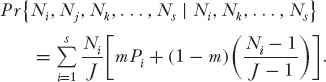
In theory, the general procedure is as follows: Let Ψ = {θ*, m*} be a particular set of trial values for the parameters. Let nr be the observed number of species with abundance r, and let Er{Ψ} be the expected number of species with abundance r from the unified theory. The log likelihood function is then given by
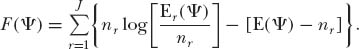
We then find the maximum of F(Ψ) as we vary Ψ. In general, relative abundance data are sparsely distributed over all possible abundances < J, so it is often more convenient to consider the expectations for grouped observations, such as in doubling classes of abundance in the case of Preston-type plots.
Unfortunately, it is only possible to write down the analytical expectations in F(Ψ) for the metacommunity case, not the local community case, and these are only practically computable for small JM. Therefore, an alternative method is required, which is to fit θ and m sequentially. The sequential fitting method works well because the estimate  is very insensitive to variation in m. Recall from chapters 4 and 5 that the locally common species on average are also the most common species in the metacommunity. Because of the stability of the law of large numbers, the local relative abundances of common species are also expected to be very close to their metacommunity relative abundances (on a percentage basis). Rare species tend to be relatively rarer in the local community than in the metacommunity (chapter 5). Therefore, in step 1, only the commonest species in the local community are used to fit the metacommunity parameter θ. For step 1, the expected metacommunity relative abundances for a random sample of size J are obtained from the algorithm given in figure 9.1. As a convenient rule of thumb, use all species more common than the median abundance to fit θ in step 1 of the estimation procedure. Once θ has been estimated, , then one proceeds to step 2 to estimate m from simulations to obtain the expected distribution of all the species, common and rare. The value of θ is fixed at , and local community dynamics are simulated for various values of m. The final estimate of m,
  , is that value which yields the maximum likelihood. This sequential estimation procedure was used to obtain θ and m for the BCI and Pasoh 50 ha plots (see figs. 5.8 and 5.9), as for the other communities discussed later in this chapter.
It is worth emphasizing that there are actually two quite different sources of variance in empirically derived distributions of relative species abundance in local communities. The first is simple sampling variance. Assuming that there exists a “true” distribution that describes the relative abundance of all species currently present in the community, then subsamples of the total community will have an associated sampling variance. This variance is the only component of variance expected from a static sampling process (e.g., the logseries or the lognormal). One can estimate the sampling variance for a dominance-diversity curve by computing the expected cumulative distribution function of the relative species abundances for the fitted values and , and then randomly sampling this distribution with a random uniform variable until the desired sample size is reached. If sample sizes are a substantial fraction of the community being sampled, then the distribution function should be created from species abundance counts (i.e., not be fractional relative species abundances), and the sampling should be done without replacement. The sampling variance is then estimated over a large number of independent trials of this random-draw procedure.
The second component of variance is perhaps the more important, and results from the dynamical process of demographic stochasticity that underlies ecological drift in the unified theory. This variance is estimated by simulating ecological drift in the local community for the fitted parameters and . One can then compute the variance in the abundance of the ranked species over an ensemble of simulation runs. In these simulation runs there is no sampling variance because all the species abundances are completely and exactly known. The total variance observed when one is sampling a real community is thus the sum of the sampling variance and the variance due to demographic stochasticity. The total variance is the measure of variation that should be used in designing statistical tests of the fit of the distributions predicted by the unified theory.
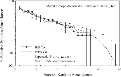
I now briefly discuss hypothesis testing about relative species abundance distributions. Typical questions likely to be asked about relative abundance include the following: Is a particular observed distribution consistent with the hypothesis of ecological drift? Are the sample distributions from two different communities statistically different? Is there excess dominance in the community over what drift alone can explain? Consider a temperate tree community example. In her book on the forests of eastern North America, Braun (1950) published numerous inventories of relative tree species abundance in many stands. Consider two mixed mesophytic forests on the Cumberland Plateau of southern Kentucky, one in Bell County and one in nearby Perry County. In the Bell County forest, the rank-1 species was sugar maple, and the second most abundant species was basswood. However, in the Perry County forest, the most abundant species was tulip poplar, and the second most abundant was beech. Based on the aggregate of a larger number of samples of stands over the Cumberland Plateau of Kentucky, I estimated the fundamental biodiversity number for the mixed mesophytic forest metacommunity. Recall that aggregating small samples from all over the metacommunity tends to overcome the effects of dispersal limitation, and the resulting distribution is expected to be closer to a logseries (chapter 6). This distribution is shown later (fig. 9.6).
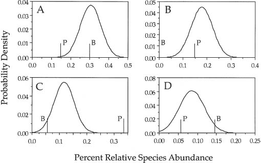
The dominance-diversity curves of the Bell County and Perry County forests are shown in figure 9.2 along with the expected metacommunity distribution for θ = 5.2 and m = 0.2, fitted by the methods given earlier. For the simulations I assumed an annual mortality rate of one percent. Based solely on the dominance-diversity curves by themselves, one can conclude that these two forests are consistent with drift and the zero-sum multinomial distribution. However, a closer examination at the species level shows that, although their dominance-diversity curves are consistent with zero-sum dynamics, these two forests are also significantly different in species composition. Figure 9.3 shows the expected distribution of relative abundance for sugar maple, beech, tulip poplar, and basswoood in terms of the percentage relative abundance of the species in the metacommunity. Beech was completely absent from the Bell County forest (panel B). The Perry Co. site also had too little sugar maple (panel A) and too much tulip poplar (panel C) to be neutrally dispersal assembled from the metacommunity. These conclusions of course depend on the assumption that the metacommunity composition of the mixed mesophytic forest has been measured accurately. A far larger regional sample would be preferable to check this assumption.
FIG. 9.2. Relative species abundance distributions for two temperate tree communities in Kentucky. The two stands were of mixed mesophytic forest on north-facing slopes a few miles apart on the Cumberland Plateau. The fitted parameter values θ and m yielded confidence intervals that completely bracketed each distribution.
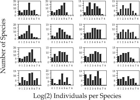
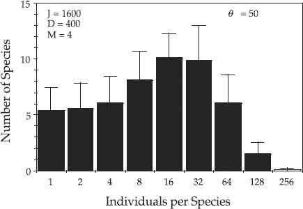
Before leaving the topic of hypothesis testing, I wish to illustrate the dangers of judging distributions of relative species abundance by visual inspection alone rather than by statistical test. Individual “snapshots” of relative species abundance distributions taken at single points in time and space may look very different from lognormals—that is, zero-sum multinomials—even when the underlying process is indeed a stochastic, zero-sum game. Depending upon the parameter values and the disturbance rate to which a community is subjected, the variance in relative abundance distributions over time can be large or small under zero-sum ecological drift. Figure 9.4 shows Preston-type plot of relative species abundance for twenty-four simulations of a model community undergoing zero-sum drift. The local community size was J = 1600 individuals, and the metacommunity had a θ of 50. The immigration rate m was 0.01, and the death rate per disturbance cycle was 400. In each run the distribution of relative species abundance was initialized as a random sample of the metacommunity. The stochastic dynamics of the community were then simulated for one thousand disturbance cycles before the relative abundance distribution was calculated. This represents 250 complete turnovers in the local community, more than adequate time for it to achieve stochastic equilibrium. The top three rows of figure 9.4 are snapshot distributions of relative species abundance for each of the first twelve simulations. The bottom row of distributions represents four of the more extreme cases that were encountered in one hundred runs. As is clear from the figure, the local community stochastic equilibrium can exhibit considerable variance, especially if the local community is subject to high disturbance rates (high turnover rates), as in the case illustrated. Many of the individual snapshot distributions do not look very much like a zero-sum multinomial, yet the underlying community dynamics do generate the expected stochastic equilibrium, zero-sum multinomial relative species abundance distribution, as shown in figure 9.5.
FIG. 9.3. Relative abundance distributions for selected individual species in 2 stands on north-facing slopes in mixed mesophytic forests in Kentucky. The curves represent the distribution of the expected percentage relative abundance of a given species based on the metacommunity relative abundances of each species, and the vertical lines are the observed percentages in the three stands. The letter B indicates the Bell Country forest, and the letter P the Perry Country forest. (A) Sugar maple, (B) beech, (C) tulip poplar, (D) basswood.
FIG. 9.4. Stochastic variation in the relative species abundance distributions of a model community undergoing zero-sum ecological drift. The metacommunity value of θ is 50. The local community size J is 1600. Immigration rate is 0.01. One quarter of the individuals are replaced per disturbance cycle. Relative abundance distributions were calculated after 1000 disturbance cycles (after 250 turnovers of the community). The top twelve panels were the results of the first twelve runs. The bottom four panels are four extreme cases found among the one hundred runs.
In a symposium on benthic marine ecology, Lambshead and Platt (1985) published a review and general critique of Preston’s hypothesis. They argued that the evidence for the pervasiveness of lognormal distributions, not only in benthic communities, but in terrestrial communities as well, was not compelling, contrary to claims in the literature (e.g., May 1975, Sugihara 1980). However, they made no formal test of goodness of fit to the lognormal. Lambshead and Platt (1985) qualitatively compared the shapes of a large number of Preston-type plots of relative species abundance distributions from various sources and concluded by visual inspection that they were rarely lognormal; or, if they were, that the lognormals were only obtained in the case of aggregated heterogeneous samples.
FIG. 9.5. Stochastic equilibrium relative species abundance distribution for the model community studied in figure 9.4. The means of one hundred independent simulations are shown. Error bars represent ±1 standard deviation. The magnitude of the error bars depends particularly on the disturbance rate (D > 1 or multiple deaths per disturbance cycle; see chapter 4).
Lambshead and Platt did not have the benefit of the unified theory in making their argument. Their failure to perform goodness of fit tests is problematic, but such tests may still fail without a dynamical hypothesis to explain the relative abundance distributions. That is, the observed variation about the expected distribution may be larger than predicted by the sample variance alone, due to the underlying stochastic demographic process. The conclusion from figures 9.4 and 9.5 is that one cannot merely visually inspect snapshot samples of the relative species abundance distribution in a community and safely conclude much of anything. The differences among the distributions in figures 9.4 are considerable despite the fact that the distributions were all produced by the identical dynamical process in a community undergoing zero-sum ecological drift. This is not to say that Lambshead and Platt were wrong about many of the communities they examined. Many communities may fail to obey zero-sum dynamics because they are so severely and frequently disturbed, that all limiting resources are not, in fact, consumed, or because the assumptions of a zero-sum game are not met.
Sampling issues and hypothesis testing regarding relative species abundance distributions are important because these distributions are widely used in attempts to measure the “health” of ecosystems (Gray 1981, Kevan et al. 1997). The rationale for these tests arises from the usually untested assumption that if communities exhibit lognormal-like distributions of relative species abundance, then they are healthier than if they do not. The unified theory provides some justification of this assumption. Relative abundance distributions are expected to deviate from the zero-sum multinomial if the disturbance rate is so severe that limiting resources are not totally saturated, so that zero-sum dynamics do not apply to the community (chapter 3). However, some researchers have concluded that finding non-lognormal-like distributions means that the communities are unhealthy. This is not necessarily so. For example, geometric-like distributions may be steady-state zero-sum multinomials in communities that are species poor simply for reasons of moderate to extreme isolation from the source-area metacommunity. The critical issue is whether the distribution remains a zero-sum multinomial, not whether it is a geometric-like or a lognormal-like multinomial.
For example, Kevan et al. (1997) compared the pollinator communities over an eight-year period in thirteen blueberry heaths in New Brunswick, Canada. Some of these heaths and the surrounding forest had been treated long-term with pesticides, whereas others were nearly pesticide free. Kevan et al. reported that they found lognormal distributions of pollinator species abundance in the pesticide-free heaths, but often did not in the pesticide-exposed heaths. They concluded that the lognormal was a reliable and sensitive diagnostic tool to diagnose ecosystem health. This may be so, but at least some of the non-lognormal distributions that Kevan et al. report are fit quite well by the zero-sum multinomial distribution.
Relative species abundance distributions have also been used to assess ecosystem health by aquatic ecologists studying benthic communities (Patrick 1968, Gray and Mirza 1979, Gray 1981, 1983). Initially it was thought that, if the lognormal was the expected distribution for undisturbed communities (Preston 1980), then departures from the lognormal, particularly toward geometric-like distributions of relative species abundance with higher dominance, could be used as sensitive indicators of disturbance, particularly by pollution (Gray and Mirza 1979, Andrews and Rickard 1980, Gray 1981, Mirza and Gray 1981, Bonsdorff and Koivisto 1982, Thompson and Shin 1983) and other environmental stresses (Gulliksen et al. 1980, Hicks 1980, Ortner et al. 1982, Soulsby et al. 1982).
As time passed and more communities were sampled, however, ecologists discovered that many unpolluted benthic communities exhibited geometric-like, not lognormal-like distributions. In these studies, most of the sample sizes were fairly small, so Hartnol et al. (1985) carried out a study to see whether relative abundance distributions would become more lognormal-like as sample sizes were increased. They took very large samples of the benthic fauna of unpolluted subtidal and tidal sands along the coast of the Isle of Man. To their surprise, even in these unpolluted sites and in large samples, they obtained geometric-like, not lognormal-like, distributions of relative species abundance. Hartnol et al. therefore concluded that departures from the lognormal could not be reliably used as an indicator of pollution disturbance or stress.
From the perspective of the unified theory, we need to qualify their conclusions. As we have seen, the theory predicts that if a local community is subject to strong dispersal limitation, then this community will exhibit a steady-state dominance-diversity curve that is geometric-like—even in the absence of any exogenous stresses such as pollution. Clearly, a stronger case for a pollution effect could be made if an actual change were observed in a given community from a lognormal-like to a geometric-like zero-sum multinomial, and if this change were associated with an alteration in pollution level. Such a change would be predicted by the theory if pollution were to cause local extinctions of some species in the community. Then, under the zero-sum rule, the surviving species in the species-poorer community would exhibit a steeper and more geometric-like dominance-diversity curve, with higher dominance of the common species. In many communities, time-series data are unfortunately not available, so whether the community has lost species, or whether there has been an increase in apparent dominance, is generally not known. However, even for single snapshot samples, it is possible to test whether the relative abundance distribution has excess dominance over that predicted by the unified theory. I will illustrate a test showing excess dominance in a tropical tree community in chapter 10.
How general is the unified theory? Until this point I have illustrated the predictive power of the theory with examples mainly drawn from closed-canopy tree communities—those with which I have the most familiarity. How well does the theory fit the data for communities of organisms that are very different ecologically and trophically from trees? In the first figure of this book, I illustrated the dominance-diversity curves of a wide variety of communities (fig. 1.1). Any durable theory of biodiversity and biogeography must successfully describe and predict dominance-diversity curves from the first principles of a dynamical theory of communities. In what follows, I merely seek to demonstrate that the unified theory does a remarkably good job of fitting many dominance-diversity distributions. However, the theory by no means fits all distributions, and therein perhaps lies the greater biological interest. I examine some failures to fit at the end of this chapter.
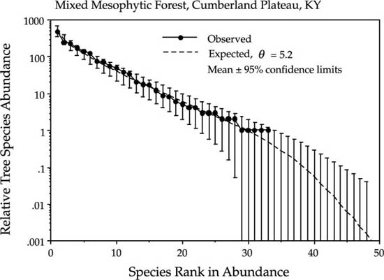
My first example is the fit of the theory to the relative abundance distribution of mixed mesophytic forest on the Cumberland Plateau of Kentucky (fig. 9.6). This distribution is based upon stands scattered over an area of approximately 13,000 square miles. The regionally pooled data, as expected, are fit quite well by the metacommunity distribution, assuming no dispersal limitation (m = 1.0). The fitted value of the fundamental biodiversity number θ was 5.2.
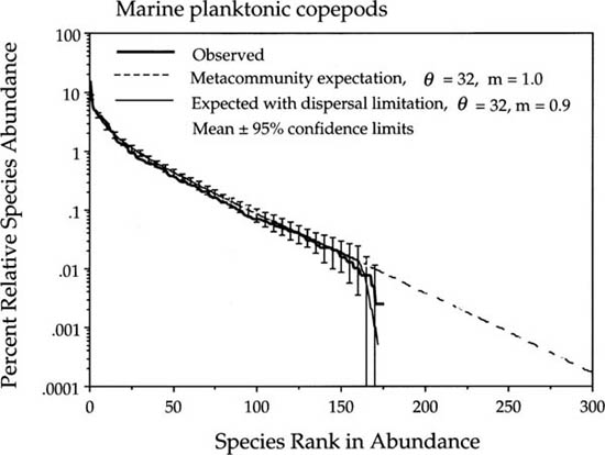
Another metacommunity distribution that is fit quite well is the set of all samples of the planktonic copepod community of the northeastern Pacific gyre (McGowan and Walker 1993) (fig. 9.7). This open-ocean copepod community is likely to be reasonably thoroughly mixed even without the pooling of plankton samples, but once again there is little hint of dispersal limitation. The estimated value of the fundamental biodiversity number θ in this community was 32, and the estimate of the immigration rate was 0.9, very close to unity.
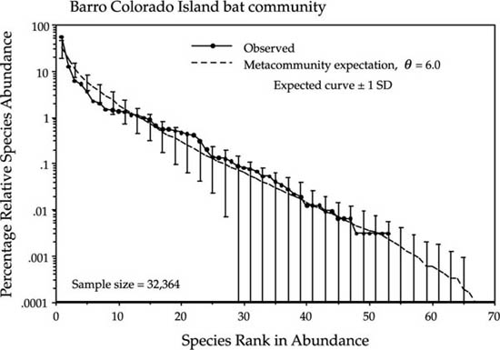
The next example is of a tropical bat community. Charles Handley and coworkers censused bats on and near Barro Colorado Island for 63 months during the decade from 1975 to 1985. Kalko et al. (1996) recently summarized these long-term studies and published dominance-diversity curves for the BCI bat community for the first time. Bats are highly mobile organisms, and one might expect that their relative abundances would therefore conform more closely to the metacommunity logseries expectation, and this seems to be the case (fig. 9.8). However, the fit to their total BCI bat community is not particularly good. Kalko et al. discuss the role of dispersal versus niche in assembling the BCI bat community, and they note that the bats differ not only in their trophic guild, but also differ in modes of foraging within these trophic guilds. There are some deviations about the expected line that are larger than those seen in earlier examples; and these deviations may reflect departures from complete zero-sum dynamics in the BCI bat community. Nevertheless, the distribution is a fair fit to a zero-sum multinomial with no dispersal limitation. The estimated value of the fundamental biodiversity number for the BCI bat community θ is 6.0.
FIG. 9.6. Fit of the metacommunity distribution to pooled data from stands of mixed mesophytic forest on the Cumberland Plateau, Kentucky. The estimated value of the fundamental biodiversity number θ is 5.2.
FIG. 9.7. Fit of the metacommunity distribution to the planktonic copepod community of the northeastern Pacific gyre, without dispersal limitation (m = 1.0) (diagonal dashed line extending off to the right), and with minor dispersal limitation (m = 0.9). Data from McGowan and Walker (1993).
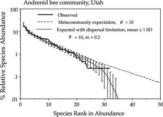
I turn now to an example of an insect community—a desert bee community in Utah. One of the most remarkable bee communities in the world is the very rich desert bee community of the American Southwest. The general view has been that many of the bee species are specialists on one kind of plant, such as one species of desert annual. More recent evidence suggests that these bees may be much more opportunistic and facultative in their foraging (Tepedino, pers. comm.). This seems reasonable given the notoriously variable annual plant community of the desert Southwest, and the dominance-diversity curve for solitary bees of the family Andrenidae supports this conclusion (fig. 9.9). Note that the dominance-diversity curve falls away from the metacommunity curve for rare species. In the unified theory, this is indicative of isolation and dispersal limitation. The estimate of m for this bee community is 0.2.
FIG. 9.8. Dominance-diversity curve for the bat community on Barro Colorado Island, Panama, and the fit of the metacommunity distribution of the unified theory, for θ = 6.0. Note that there is no evidence of dispersal limitation in these data. Part of the reason may be that these abundance represent capture records through time, so that there is a time factor that may have helped overcome the dispersal limitation of some species. Data are from Kalko et al. (1996).
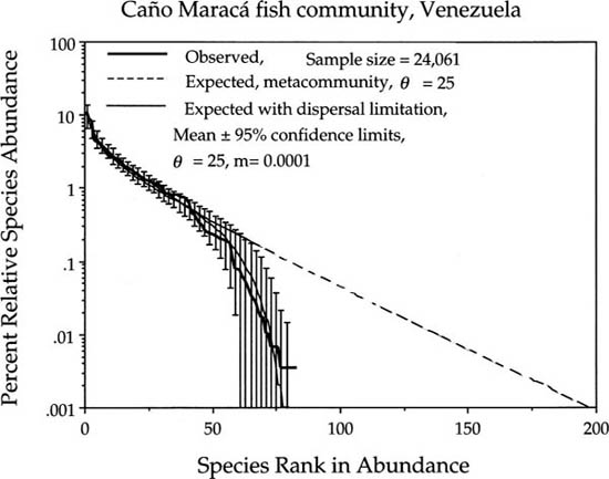
A community which shows evidence of extreme isolation and dispersal limitation is the freshwater fish community of Caño Maracá in the headwater tributaries of the Rio Negro in southern Venezuela (Winemiller 1996). Very large fish collections over a number of years have produced a detailed record of relative species abundances, even for very rare species (fig. 9.10). The steep falloff of the dominance-diversity curve from the metacommunity curve begins at about fifty species. The rarest 40% of the species collectively constitute just 1.95% of all individuals. The value of θ estimated from the common species is 25. The estimated probability of immigration, m, is very small—only one in 10,000 births for this headwaters fish community.
FIG. 9.9. Desert bee community, family Andrenidae, in Utah. The community has an estimated θ of 10 and also shows evidence of dispersal limitation (m = 0.2). Data courtesy of Vince Tepedino of Utah State University and the USDA Apis Research Service.
It might not be surprising that a tropical river headwaters fish community is so isolated, but what about a bird community? Richard Holmes has been studying the long-term dynamics of the bird community in the forests of Hubbard Brook, New Hampshire, for more than 30 years (Holmes et al. 1986)(fig. 9.11). Many of the Hubbard Brook bird species are summer breeding residents and winter migrants. I examined the relative abundances of the subset of species that are primarily insectivores, assuming that these species would represent a guild that might reasonably be expected to obey zero-sum dynamics. The data are very well fit by a zero-sum multinomial with θ = 5.0 and m = 0.2. This suggests that approximately one out of every five insectivorous birds in the community is an immigrant and, conversely, that four out of five birds were born locally in the Hubbard Brook forest.
FIG. 9.10. Tropical freshwater fish community in a system of tributaries in the upper watershed of the Rio Negro. Note the extreme degree of isolation evident for this fish community: the estimate of the probability of immigration per birth m is only 0.0001. The estimated fundamental biodiversity number θ is 25. Data courtesy of K. Winemiller.
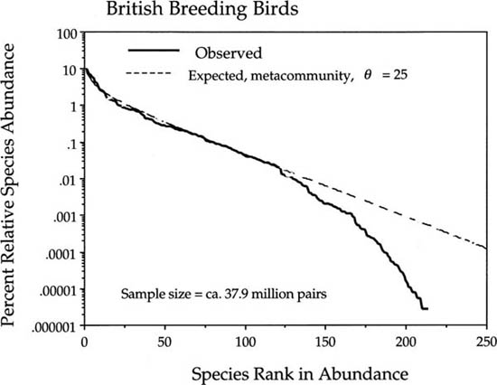
The final example is the dominance-diversity curve for the entire avifauna of Great Britain (Gibbons et al. 1993), which I presented as a Preston-type plot in chapter 2 to illustrate the shape of the zero-sum multinomial (fig. 2.6). When plotted as a dominance-diversity curve, we observe the now familiar phenomenon of the departure of the observed distribution from the metacommunity expectation for rare and very rare species (fig. 9.12). I show this distribution primarily to make the point that dispersal limitation can be detected on arbitrarily large spatial scales, as for example, on the scale of Great Britain. There are many problems with the precision of estimating bird population sizes in such a large area (Gibbons et al. 1993). However, in the well-studied British avifauna, it is almost certainly the case that the absolute abundances of the rarest species are better known than the absolute abundances of the commonest species. This means that we can put considerable confidence in the shape of the dominance-diversity curve at the rare end of the distribution. The common end is also well determined for purposes of a dominance-diversity plot because relatively large absolute errors in estimating the abundances of common species become insignificant on a log scale (fig. 9.12). It is possible to fit the metacommunity distribution to these data, which yields a value of the fundamental biodiversity number θ of 25. However, I was not able to fit the entire community of 37.9 million breeding pairs of birds for the dispersal limitation parameter m because the community size is too large for my computer.
FIG. 9.11. The long-term average dominance-diversity curve for 15 species of insectivorous birds in the summer breeding bird community of Hubbard Brook, New Hampshire, USA. The estimated value of the fundamental biodiversity number θ is 5.2, and the estimated per capita probability of immigration m is 0.2. Data from Holmes et al. (1986).
FIG. 9.12. The dominance-diversity curve for the entire British breeding avifauna. The estimated fundamental biodiversity number θ is 25. Data from Gibbons et al. (1993).
I conclude this chapter with a discussion of the robustness of the unified theory of biodiversity and biogeography. By robustness I refer to the ability of the theory to withstand violations of its assumptions and still be predictively useful. A case in point is the excellent fit of the theory to the relative species abundance distribution of the entire British breeding avifauna, given just above (fig. 9.12). The fit to the British avifauna, which includes everything from seabirds to raptors to warblers, suggests that, at least on such macroscopic scales, the differences in ecology among the species become obscured by biogeographic factors operating on very different spatial and temporal scales. Moreover, differences in ecology may tend to be overwhelmed by the absolutely vast differences in relative species abundance represented by the distribution, which ranges over seven orders of magnitude, from species having a single breeding pair to species with tens of millions of breeding pairs. Such a good fit may also be an exception, however. It is too early to say. Certainly there is abundant and growing evidence that energetic and biomechanical scaling laws exist that dictate that the body size of species will be strongly and negatively correlated with landscape-level species abundance in many taxa (e.g., Brown 1995). At this early stage in the theory’s development, it is impossible to give definitive answers to questions about its robustness. Nevertheless, there are still some useful things that can be said about robustness at this point.
First, we can dispense with the concern that the theory may “fit everything”—a concern raised, for example, by the excellent fit to the entire British breeding avifauna. A neutral theory that fitted everything would not be very useful because it would fail to instruct us about the assembly of natural communities. Exactly when and how a good formal neutral theory fails should be as interesting, if not more so, as when and how it succeeds.
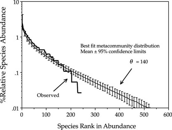
Fortunately, it is not difficult to find communities in which the dominance-diversity curve predicted by the unified theory does not, in fact, fit the data. For example, it fails to fit the relative abundance data for all birds censused in a 10 ha plot of forest in Manu National Park, Amazonian Peru (Terborgh et al. 1990). Like the British avifauna, this survey included all taxa, irrespective of ecology, from hummingbirds to guans. But unlike the British avifauna, the distribution of Manu birds deviates significantly from the best-fit theoretical metacommunity distribution. The Manu sample was of a very local bird community, in which the range in relative abundance was much smaller (only two orders of magnitude) than in the example of all breeding birds of Great Britain. Whatever the cause of differences in fit, the theory does not fit the observed distribution for Manu (fig. 9.13).
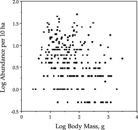
Attempts to fit the metacommunity distribution to the common species failed in two interesting ways. If the fundamental biodiversity number is fit to the fifty most abundant species, then there is an excess of abundance in the midrank species over expected abundances. On the other hand, if the midrank species are also included in the set of species fit by the metacommunity distribution (the 150 most abundant species), then the most abundant species display excess dominance. That is, the observed abundance for the most abundant species is significantly greater than the predicted abundance of these species by the metacommunity distribution. We can begin to explore some reasons for the lack of fit in this case. A major violation of the assumption of zero-sum dynamics is a likely candidate. Terborgh et al. (1990) also presented data on the average masses of the different species in the Manu forest. It is interesting that there is only a weak negative and nonsignificant correlation between abundance and body mass in these data (R2 = 0.096) (fig. 9.14). Among other things, this lack of correlation may reflect the fact that the spatial scale of resource dependence that determines bird abundances is very different among different trophic guilds, so that the 10 ha spatial scale of reference is inappropriate for all species. For example, raptors exploit prey resources over a much larger area than 10 ha, whereas many small insectivores might spend their entire lives in the 10 ha plot. This underscores the fact that one of the major challenges in testing the unified theory is determining the appropriate spatial and temporal scales for defining both local communities and the metacommunity. This may be a far easier task in general for communities of sessile organisms.
FIG. 9.13. The observed dominance-diversity curve (heavy line) for all species of bird censused in a 10 ha sample of mature forest in Manu National Park, Peru. The best fit metacommunity distribution yields a θ of 140. However, the metacommunity distribution fails to predict the high abundance of the midrank species. No attempt was made to fit the probability of immigration, m in this case, although it is clear that dispersal limitation does affect the curve for species that are rarer than rank 150. Data from Terborgh et al. (1990).
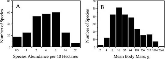
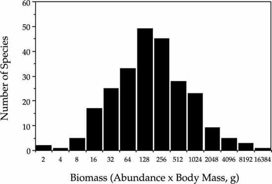
The fact that biomass and abundance are largely decoupled in this bird community is further supported by the following observation. The distribution of relative species abundance is negatively skewed, as predicted by the zero-sum multinomial (fig. 9.15A). However, the distribution of body mass is positively skewed even as a log-transformed Preston-type plot (fig. 9.15B). The total community biomass distribution can be computed by plotting the distribution of the product of mean body mass times the species abundance per 10 ha. This distribution of the biomass of total bird species populations in the 10 ha Manu plot is nearly perfectly lognormal in shape (fig. 9.16). This finding suggests that there is little reason to expect a strong relationship between body size and abundance in local communities where the resources supporting that community may or may not be completely local. The whole issue of body size has not been treated at all thus far by the unified theory. The linkages between theories of body size scaling rules, zero-sum dynamics, and the unified theory are likely to be very fertile areas for future theoretical exploration, but this lies beyond the scope of the present book.
FIG. 9.14. Lack of relationship between average body mass of bird species in a 10 ha plot in Manu National Park, Peru, and the abundance of the species in the plot. Note that a few species have estimated abundances in the 10 ha plot that are less than unity. These were species that may not have breeding pairs in the plot. Data from Terborgh et al. (1990).
FIG. 9.15. Distributions of bird species abundance (A) and of mean body mass in grams (B) for the bird community in the 10 ha plot in Manu National Park, Peru. Data from Terborgh et al. (1990).
FIG. 9.16. Distribution of total bird species population biomass in a bird community in Manu National Park, Peru, expressed as abundance per 10 ha times mean body mass in grams. Data from Terborgh et al. (1990).
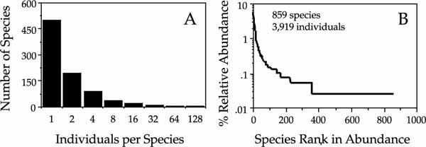
I now illustrate one more case in which there is a poor fit of the unified theory. These are data on rain-forest canopy Coleoptera collected and identified by Nigel Stork and colleagues from the canopies of ten trees in Borneo (Stork 1997). These samples, and others on chalcid wasps not shown, are characterized by an enormous fraction of singleton species. In the sample illustrated in figure 9.17, 499 out of 859 species (58%) were collected only once. At the other extreme of abundance, the top ten most abundant species constitute a third of all individuals (32.2%). The unified theory in its present form fails to fit these data. If we use the top ten species to estimate the fundamental biodiversity number, the resulting metacommunity curve is far too steep for the observed dominance-diversity curve, and the fitted θ considerably underestimates the species richness observed in the sample. One explanation for this failure might be that a very large fraction of the singletons represent nonresident species that were temporarily resting on the sampled trees at the time of the collection. Stork (1997) states that many of the extremely rare species probably do not feed on the tree species from which they were collected. There are no host plant records to support this speculation, but it is a reasonable hypothesis. Most of the beetle species are extremely small, and they are likely to be capable of long-distance dispersal, carried by the wind. The data in figure 9.17B are exactly what one would expect if the dispersal kernels of these beetles were highly leptokurtic with extremely long “fat” tails, extending far away from individual host trees.
FIG. 9.17. Relative abundance distributions for Coleoptera collected from 10 trees in a rainforest in Borneo. (A) A Preston-type plot showing the enormous number of species collected only once. (B) The corresponding dominance curve. There were 859 species found among 3919 individuals. Data from Stork (1997).
It should be noted that that the data in figure 9.17 are not intrinsically incompatible with neutral theory. In a more refined, spatially explicit version of the theory, we could build in a strongly leptokurtic dispersal kernel that would have the effect of increasing the proportion of rare, long-distance dispersers in local communities. This dispersal function could apply equally to all species, and the theory would still remain completely neutral, according to the definition of neutrality given in chapter 1.
The key assumptions of the unified neutral theory of biodiversity and biogeography really boil down to only two. The first is that all species are identical on a per capita basis in their probabilities of birth, death, and dispersal. The second is that these species are locked in a life-or-death zero-sum game competing for the same, shared, limiting resources. How robust is the unified theory to violation of these assumptions? Ironically, if one believes that most ecological communities are fundamentally niche assembled, then the answer must be “very robust,” because the theory does a remarkably good job of describing local and landscape patterns of biodiversity across a wide variety of communities. I discuss robustness further in the concluding chapter 10 because I believe that understanding why the neutral theory does so well in spite of manifest differences among species also provides the key to reconciling neutral, dispersal-assembly theory with niche-assembly theory.
1. There are two important statistical distributions in the unified neutral theory. One is the asymptotic logseries distribution for the metacommunity under point mutation speciation; the other is a new statistical distribution, the zero-sum multinomial, which arises in the local community under dispersal limitation from the metacommunity. The zero-sum multinomial is also the metacommunity relative abundance distribution under random fission speciation.
2. Fitting the fundamental biodiversity number and the dispersal rate currently requires simulations for any reasonable-sized community. Publication of an extensive tabling of the zero-sum multinomial distribution is planned to aid in hypothesis testing.
3. A fast algorithm for computing the expected metacommunity relative abundance distribution under point mutation speciation is given.
4. In general, the fundamental biodiversity number will tend to be underestimated from local samples of relative species abundance. The underestimation is hard to estimate a priori because it depends on the amount of dispersal limitation. However, better estimates of θ are obtained if the fitting is restricted to the common species in the local community, which are more likely to be widespread metacommunity species. The best estimates of θ are likely to be obtained from pooling samples collected all across the metacommunity.
5. The theory fits the relative species abundance data from a diverse array of communities, from marine planktonic copepods to tropical trees. However, there are many distributions that it does not fit well for expected biological reasons, particularly for violations of the zero-sum rule.
6. Therefore, the theory is expected to be useful in testing the importance of ecological drift, random dispersal, and random speciation in structuring natural communities.