Chapter 5

Darwinian Evolution

Let us begin the post-Enlightenment era with the giant gap between the first atomist, Democritus, and the modern atomist, Mendeleev.

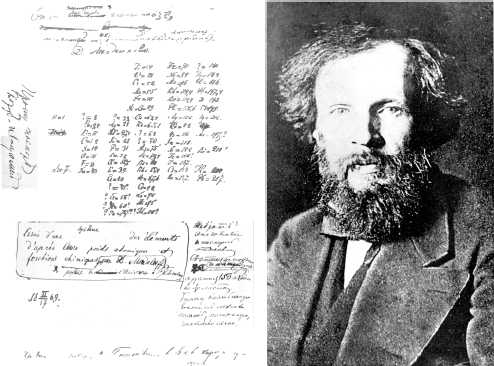
Dmitri Ivanovich Mendeleev (08.02.1834–02.02.1907) was a Russian chemist and inventor. He is best known for periodic table in his name. Russian physicist Andrei Matlashov informs that Mendeleev was born in the village of Verkhnie Aremzyani, near Tobolsk in Siberia, to Ivan Pavlovich Mendeleev (1783–1847) and Maria Dmitrievna Mendeleeva (née Kornilieva) (1793–1850). Ivan worked as a school principal and a teacher of fine arts, politics and philosophy at the Tambov and Saratov gymnasiums. Dmitri’s grandfather, Pavel Maximovich Sokolov, was a Russian Orthodox priest from the Tver region.

Mendeleev was raised as an Orthodox Christian, his mother encouraging him to “patiently search divine and scientific truth”, but Mendeleev seemed to have very few theological commitments. Mendeleev’s son Ivan said, “. . . from his earliest years Father practically split from the church–and if he tolerated certain simple everyday rites, then only as an innocent national tradition, similar to Easter cakes, which he didn’t consider worth fighting against. . . . Mendeleev’s opposition to traditional Orthodoxy was not due to either atheism or a scientific materialism”.1 Rather, he held to a form of romanticised deism about God not involving Himself in human affairs even if He created the world. At age 21 in 1855, he moved to the Crimean Peninsula on the northern coast of the Black Sea in order to cure his tuberculosis. In 1857, he returned to S. Petersburg with fully restored health. He got a tenure at St. Petersburg University in 1867 and started to teach inorganic chemistry.

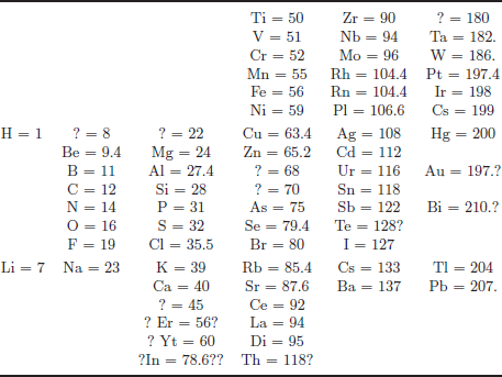
During 1868 and 1870, Mendeleev wrote the two-volume textbook, Fundamentals of Chemistry. After finishing the first part at the end of 1868, he was on a two-week business travel from February 17, 1869, looking for dairy farms. He was under the extreme Zeitnöt (time pressure) with the desire to finish the table needed for the next lectures from March 1, 1869, at St. Petersburg University and to fulfil the business duty, but this was the time when he made his most important table. At this time, he had the basic idea of making a table by placing chemical elements along the atomic weights like arranging cards by the suits, and the first part dealt with alkali metals and haploids. He remembered all 63 elements by heart and placed 43 on the table and 20 on the margin, trying to put them into the table. On February 17, 1869, he placed all 63 elements on the table without any element in the margin, as shown in Fig. 1. But, question marks appear on Table 1.

Another person classifying chemical elements in the early 1860s was Lothar Meyer who listed 28 elements classified by their valence, but not with atomic weights. Mendeleev was unaware of Meyer’s work going on in the 1860s.² As he attempted to classify the elements according to their chemical properties, by atomic weights, he noticed patterns that finally led him to postulate his periodic table. According to his friend, Inostrantzev, he claimed to have envisioned the complete arrangement of the elements in a dream, “I saw in a dream a table where all elements fell into place as required. Awakening, I immediately wrote it down on a piece of paper, only in one place did a correction later seem necessary,” as quoted by Kedrov on the occasion of the fiftieth anniversary of the death of Mendeleev. By adding additional elements following this pattern, Mendeleev placed them in a “periodic” way and arranged them according to their atomic mass, as shown in Fig. 1,³ so that groups of elements with similar properties fell into horizontal columns (now, chemical “groups” are shown vertically in contrast to their horizontal format in Mendeleev’s table). Mendeleev’s version had period 8 for 63 elements.

Figure 1: Mendeleev’s handwriting taken from Karpov’s talk.

On March 6, 1869, he made a formal presentation of this table to the Russian Chemical Society, titled The Dependence between the Properties of the Atomic Weights of the Elements, which described elements according to both valence and atomic weight. The number of natural elements are 92 with uranium being the 92nd. Now, artificial elements with valence exceeding 92 are manufactured and so far Atomic Number 115 has been observed. Hints of Nature to atomists have been revealed first by the regularity as Mendeleev noticed and later by Murray Gell-Mann in his 1960s eight-fold way of hadrons.

Table 1: Mendeleev’s Tentative System of Elements (63 elements) written on February 17, 1869 as Fig. 1.

When Mendeleev told the story of his dream to Inostrantzev, he was quoted to have said “after three sleepless nights”, but from many sources, the writing of Fig. 1 was a single-day event on February 17, 1869 under the extreme Zeitnöt.

On the back of the letter for the day’s official program, Mendeleev wrote, during the breakfast time, his first calculations upon comparing the group of alkaline metals and other groups. This might have been based on his dream of the previous night. His coffee mug was on the paper and left a “trifle” mark on the letter. Historians should pay attention to such “trifles” to convince people that the discovery was a single-day event, as mentioned by Kerdrov. But, this story was in echo (in another aspect) with the second author’s frequent teachings to the university students to prepare enough for the exciting moment similar to a lion that frequently sharpens his teeth for the next hunt. Without preparation, he would not get profit from such jolting moments. The exact person in question Mendeleev, had no illusions. What he needed was just the jolt of February 17, 1869.

Mendeleev was a preservationist of Earth, as he remarked that burning petroleum as a fuel “would be akin to firing up a kitchen stove with bank notes”,4 and hence a true atomist. It is known that he was against the scientific claims of spiritualism. He bemoaned the generally accepted spiritualism in Russia and its negative effects on the study of science.

In the 19th century, thermodynamics played a major role in the evolution of theoretical physics, leading to the profound and slightly mysterious concept of entropy. The French physicist who was the father of thermodynamics and whose work started the intellectual path towards entropy was Sadi Carnot (1796–1832). In an 1824 book, Carnot began a new field of research, thermodynamics, and his Carnot Cycle was what later led the German physicist Clausius to the idea of entropy in 1865. The Carnot Cycle is a simple model which mimics the operation of a steam engine.

Rudolf Clausius (1822–1888), a German physicist and mathematician, may justly be regarded as the father of entropy. He was initially inspired by the Carnot Cycle which requires the equality of a ratio of heat energy to absolute temperature for the hot and cold heat reservoirs.

In the presence of irreversible processes in a variant of the Carnot Cycle, one would, instead of this equality, arrive at an inequality which gives rise to the second law of thermodynamics that entropy denoted S (closely related to the ratio (heat)/(temperature)) cannot decrease. This led Clausius to a definition for incremental entropy as the exact differential near to thermal equilibrium and thence to the second law of thermodynamics dS ≥ 0. We emphasise that Clausius’s discussion is appropriate only near to thermal equilibrium because a thermally insulated box of ideal gas with an unlikely initial condition, e.g. all the molecules in one corner, will rapidly increase its entropy to approach thermal equilibrium despite the fact that δQ ≡ 0. Clausius denoted entropy by S in honour of Sadi Carnot.

Clausius enunciated two laws of thermodynamics as follows:

1.The energy of the universe is a constant.

2.The entropy of the universe tends to a maximum.

Kinetic theory shows how the P, V, T thermodynamic variables can be related to the average motions of the molecules using statistical mechanics. The question following Clausius’s work was how to relate the state function S to microscopic variables. Ludwig Boltzmann (1844–1906) was the physicist who solved this problem. He had no experimental evidence for molecules; this had to wait 30 more years until the explanation of Brownian motion in 1905 by Einstein and Smoluchowski.

Regarding Boltzmann, few people were convinced of the reality of atoms and molecules before the last year of his life. Further, his statistical, hence inexact, second law of thermodynamics was strongly criticised by Maxwell who, although he believed in atoms and molecules, never accepted Boltzmann’s 1872 idea of an inexact law of physics. Boltzmann appreciated that his law was so unlikely to be violated that it might as well have been exact.

Another severe criticism came from the distinguished French mathematician Henri Poincaré (1854–1912) who proved a rigorous recurrence theorem which states that all systems must return eventually to their original state. Boltzmann understood that the timescale involved in Poincaré recurrence is far too long to be physically relevant. In any case, Boltzmann’s lack of recognition in the physics and mathematics communities may have contributed to his suicide at the early age of 62 in 1906.

Boltzmann defined as microstates all the possible arrangements of microscopic variables corresponding to a given fixed set of macroscopic or thermodynamic variables whereupon he defined S = k ln W, where W is the total number of microstates. This is one of the most celebrated equations in all of physics and is written as an epitaph on Boltzmann’s tomb in Vienna Central Cemetery.

For an ideal gas, the maximisation of entropy S means that in the state of thermal equilibrium, there is the maximum uncertainty in the molecular motions. We can equivalently say that there is the greatest disorder in thermal equilibrium and hence this entropy is a measure of disorder when disorder is suitably defined.

The H theorem of Boltzmann in 1872 is central to physics although even now in 2019 we are told that it cannot be rigorously proved mathematically because, at least far away from equilibrium, it is unknown whether solutions of the Boltzmann transport equation have sufficient analytic smoothness. Nevertheless, the H theorem shows how starting from reversible microscopic mechanics, one can arrive at non-reversible, in a statistical sense, macroscopic dynamics. It explicates the second law of thermodynamics that the entropy of an isolated system cannot decrease. As we deviate from thermal equilibrium, however, the second law must be generalised by the use of the so-called fluctuation theorem.

The paper by Boltzmann in which he proved the H theorem has been studied and criticised probably as much as any physics paper. One interesting critique is by Von Neumann (1903–1957).

The reason why the H theorem of Boltzmann is far more powerful than the infinitesimal definition of dS by Clausius is that it proves that dS ≥ 0 for non-equilibrium systems assuming only the Boltzmann transport equation, the ergodic hypothesis and Stosszhalansatz which is German for molecular chaos that neglects correlations.

What is clear about S(t) for a box of ideal gas is that with thermal equilibrium S(t) is a maximum. From the definition of S, this implies that the number of microstates corresponding to the thermally equilibrated system is the highest and that the molecular motion is therefore the most disordered.

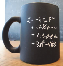
Figure 2: John Ellis wrote the SM equations on a CERN mug.

The H theorem encapsulates this edifice of 19th-century knowledge sufficiently to progress with some confidence from a box of ideal gas to more interesting cases such as the early universe, where the concept of the entropy of the universe may be useful.

Some 300 miles north from Kiderminster, James Maxwell (1831–1879) was born in Edinburgh, Scottland. His contribution in kinetic theory of gases is paramount but his equations of 1861, On Physical Lines of Forces,5 unifying electricity and magnetism, outstand it. In the subsequent paper of 1865, A Dynamical Theory of the Electromagnetic Fields,⁶ we can count eight equations that we use today. In the modern agreement, one equation, the first line on a CERN mug shown in Fig. 2, is enough and even contains more. The only other correct equations known before World War II and still used by modern atomic theorists are Einstein’s gravitational equation, not shown in the mug, and Dirac’s equation shown in the second and third lines for quarks and leptons.

Breaking of the 20th century opened the gate to a long tunnel leading to the modern day atomic theory. In 1896, Henri Becquerel (1852–1908) noticed β-spectrum from the radioactive nuclei, which is a beam of the fundamental particle electron. A year later, John Thompson (1856–1940) showed that cathode rays were composed of previously unknown negatively charged particles which he calculated must have bodies much smaller than atoms and a very large charge-to-mass ratio. Now, Thompson is credited for the discovery of electron while Becquerel is credited for observing the weak interaction phenomena for the first time. From the study of blackbody spectrum, it was necessary to introduce the quantum idea of Max Planck (1858–1947) with a new fundamental constant of Nature with his name attached, h. When any physics calculation involves h, it is a quantum phenomena. This constant being so important, modern atomists mostly researching quantum phenomena agreed not to write h explicitly. Now, Planck rests at the Göttingen Cemetery with Max Born and several other German Nobel laureates. In this breaking period, a particle introduced with h for the first time was by Albert Einstein (1879–1955) on the nature of already known Maxwell’s electromagnetic wave. In the visible light range, it is called “photon” (“-on” means a particle physicist’s favourite naming system for a fundamental particle), which (not the relativity theory) awarded him the Nobel prize.

Steven Weinberg7 classifies the giant physicists into sages and magicians: “sage-physicists reason in an orderly way about physical problems on the basis of fundamental ideas of the way that nature ought to be . . . magician-physicists who do not seem to reason at all but jump over all intermediate steps to new insights about nature.” Early quantum theorists and the modern atomists are mostly magicians. Albert Einstein and Wolfgang Pauli are considered to be sages and Werner Heisenberg, Erwin Schrödinger, and Niels Bohr are considered to be magicians. In proposing particles, both Einstein and Pauli worked like magicians for photon in 1905 and for neutrino in 1930, respectively.

Formulation of quantum mechanics in the mid-1920s was a revolution in atomic physics, even more so than Newton’s classical mechanics. Quantum mechanics provided the notion of identical particles that was one of the postulates of the Greek atomists. A brief history until 1926 is as follows. After Niels Bohr declared the allowed atomic orbits in 1913, it was the problem of physicists to understand the energy levels of the Bohr atom. It occurred to Werner Heisenberg in 1925 during his escape to Heligoland Island in North Sea that Bohr’s atomic orbit is not observable and hence one can consider a scheme with only measurable numbers, a thread leading to his great achievement. The final outcome of his study with only measurable numbers such as position and momentum is now known as matrix mechanics, which is one version of quantum mechanics. There is another formulation called wave mechanics, known as Schrödinger’s work, which have become the working ground of theoretical chemistry. The idea is based on the wave function. For any observable, there exists the wave function denoted as Ψ.

The wave function idea was first introduced by a French physicist, Louis Victor Pierre Raymond de Broglie, 7th duc de Broglie, in 1923. He postulated the wave nature of electrons, giving the electron wavelength proportional to the inverse of its momentum and suggested that all matter has wave properties. There is an anecdote on how Schrödinger is related to the wave function. In 1921, Schrödinger at age 32 moved to the ETH Zürich, where the leader was 37 year old Peter Debye (1916–2012). In 1925, de Broglie gave a seminar on his electron wave at ETH. After the seminar, Debye asked de Broglie, “I know that all waves have the wave equations that they follow. If yours is matter wave, what is your equation of motion?” when de Broglie could not answer the question, Debye turned to Schrödinger and told him,8 “Rather than going out for hiking, get the equation of de Broglie’s.” In 1926, Schrödinger happily obtained his equation for matter waves, which included a phase i unlike in all other previous wave equations.

The interpretation of the wave function based on the work of the German mathematician at Göttingen, Max Born (1882–1970), is that it is the probability amplitude, i.e. the probability to find a matter particle is proportional to |Ψ|². Göttingen, the centre of the Germany map, was the centre of new physics in 1920s. Heisenberg, Dirac, and Oppenheimer came to Göttingen and were guided by Max Born, whose tombstone at the Göttingen Cemetery reads pq − qp = where h is the Planck constant. This is Heisenberg’s uncertainty relation and it seems that the Göttingen group considered it as their work. The probability interpretation invites transformations which do not change the probability, i.e. the electron number is not created or destroyed. If we multiply a phase to the wave function, e^iαΨ, the probability |Ψ|² remains the same. Thus, in quantum mechanics, we consider only the probability conserving transformations. A generalisation of e^iα is the unitary transformation where F_i is called the generators of the unitary transformation. In this regard, Chen Ning Yang called quantum mechanics phase mechanics.

Heisenberg introduced the notion of uncertainty principle. In mathematics, any well-behaved function in a definite region can be written as a linear sum of functions of a complete set in the defined region. For example, for x in the region x ∈ [0, 2π), sin x can be written as a Taylor series: sin x = x − + · · · since {1, x, x², . . .} is a complete set. If x denotes the coordinate of the measurable displacement, any wave function can be a function of x only, Ψ(x). But, the linear momentum in classical mechanics of a particle at x is To relate to this classical relation, it is noted that is related to x but not as a function of x only. It involves the derivative with respect to t. For an x-dependent function Ψ(x), the t dependence can be only by the derivative for Ψ(x) now a function of t through x(t). So, we consider only differentiable functions for Ψ(x(t)). Differential operation acts on the function Ψ(x(t)). With this definable setup, we can calculate pΨ(x(t)). But, in the operation p(xΨ(x)), p with the act of differentiation just does not go through x. Therefore, (xp − px)Ψ(x) = Ψ(x), introducing a non-vanishing commutator for x and p. (xp − px) is denoted as the commutator [x, p] written on the tombstone of Max Born.

One complete set of functions in the interval x = (−π, +π] is {e^inx, n = integer} in terms of which we can expand any differentiable function Ψ(x), which is called Fourier series. This can be generalised to a continuous variable, n → k (or p), which is called “Fourier transformation”. As commented before, this transformation using e^ikx is the probability conserving transformation. Explicitly, the Fourier transformation is Ψ′(p) ∝ ∫ dx e^ixp/ħΨ(x) where ħ has the dimension of = [energy · time]. Because the wave function involves two measurable variables x and p with the locked-up phase e^ixp/ħ, they have the uncertainty relation [x, p] = iħ, where ħ ≡ h/2π. If two observables do not have that locked-up phase, they do not have the uncertainty relation. In most undergraduate textbooks on quantum mechanics, therefore, the uncertainty relation is exercised in terms of Fourier transformation.

On the right-hand side of the uncertainty relation, the so-called Planck constant ħ describes how visible is the quantum effects are. The action unit is represented in units of the Planck constant ħ.9 If the action is order 1 compared to the Planck constant ħ, then the quantum effect is manifest. If the action is much larger than 1 compared to the Planck constant ħ, then the quantum effect oscillates out. Since the Planck constant ħ has the unit [energy · time], (time) × (energy) can appear in the phase in the unitary transformation Ψ′(p) ∝ ∫ dx e^−itE/ħΨ(x). Therefore, the energy–momentum relation of observables E and p in classical mechanics, E = + V(x), written on wave function introduces i on the left-hand side of the Schrödinger equation. The relativistic generalisation of the Schrödinger equation is the Klein–Gordon equation for spin-0 waves and the Dirac equation for spin- waves.

One crucial part missed by the earlier atomists (Democritus, Epicurus, Lucretius, Dalton, Mendeleev, Bohr) is the concept of rotation of indivisible atoms or particles. Atoms could not be seen with the traditional light microscopes invented in the 17th century. As mentioned in Chapter 1, Robert Hooke observed the “teeth of time” in 1655 with the light microscope. The scanning tunnelling microscopes of today, imaging surfaces at the atomic level, cannot see the rotation either. From time to time these days, we watch in the TV news the current nanotechnology achievements, showing images of the sizes larger than a 10-millionth cm, roughly 10 times larger than the sizes of atoms. Even popular physics books written these days¹⁰ do not emphasise the importance of rotation of elementary particles mainly because the “V–A” quartet had not been credited by the Nobel Committee. Now, the Committee lost its chance since all the four (Feynman, Gell-Mann, Marshak, and Sudarshan), involved in the initial discovery of interactions related to the rotation of fundamental particles, passed away. In the beginning of Chapter 8, we discuss more about their ideas.

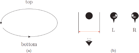
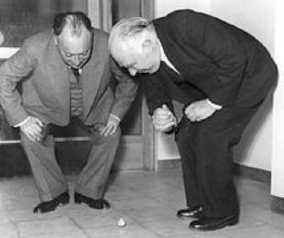
Rotations of Sun, Moon, and Planets in their orbits were known to Greeks, but the concept of rotation was not used in their atomic theory. Even if the idea were used then, this kind of orbit could not be successfully embedded in their atomic theory. Figure 3(a) shows an orbital rotation for one cycle. If one looks at it, it is rotating in the counterclockwise direction from top and clockwise direction from bottom. Therefore, clockwise or counterclockwise rotations of an orbital rotation of a star in the heaven are not distinguished. But, if a top is rotating, then one can say whether it is rotating clockwise or counterclockwise; see Fig. 4 showing as Wolfgang Pauli and Niels Bohr watch a rotating top. In fact, the rotation of the top is an orbital rotation because each point in the top rotates along its orbit of rotation. The clockwise or counterclockwise sense of Pauli and Bohr was because they could not see the rotation from under the floor.

If rotation of an electron around nucleus, which Niels Bohr modelled for the Hydrogen energy spectrum, is considered, then again the rotational orbit is the first guess. But, if the size of something is very small for our ability (the range of red arrows) of measuring its size, as shown on the left-hand side in Fig. 3(b), the story is different. In this case, there is no way to convince ourselves about the clockwise or counterclockwise sense of rotation of the object. The size of an object must be covered in the atomic theory.

Figure 3: Rotations: (a) rotation along an orbit; (b) consideration for possible rotations of an atom, and L and R from the top view.

Figure 4: Wolfgang Pauli, the inventor of word “spin”, and Niels Bohr, the inventor of his atomic model, watching a spinning top.

Peeling the onion structure of matter, we end up with the indivisible atoms. In fact, Democritus’s atom must be interpreted as being smaller than Bohr’s atom by the modern atomists. The size is roughly the same distance that light travels along its size. Here, we recognise that Einstein’s famous formula E = mc² is useful, where he claims mass is energy. As anybody experiences when he/she tries to divide some number by a very small number, 0 is very different from a non-zero number however small that number might be. Einstein considered mc² (with the velocity of light c) as the rest mass. When a particle moves, its energy is bigger than this rest mass energy. Because the rest mass is the smallest energy that the particle can possess, let us express energy as E = mc²+(something) and measure the traversing time. The distance corresponding to the smallest energy, i.e. E = mc², is called the Compton wavelength to remember Arthur Compton who detected the electron scattered by light for the first time. For light, it is very strange. Light, radio waves, microwaves by which we receive TV broadcasts, X-rays, and gamma rays all travel with the same velocity, 380,000 km/s, at the sea level in England and Korea. Einstein gives the velocity or momentum of a particle as p = which is the same as E = mc²+(something). Since all kinds of electromagnetic waves travel with velocity c, mass of light or more generally mass of electromagnetic waves must be zero. The exact zero mass has a great significance, as will be discussed further in Chapter 8. The time measured by light travel has a physical significance. If a particle has mass m and has an extended Compton wavelength size λ_c, the time required to traverse the particle is λ_c/c, and Compton defined the distance in terms of just one number, the rest mass.

In 1925, the Zeeman effect that Bohr’s energy levels are split when atoms are placed in the magnetic fields was known. In classical mechanics, as mentioned above, angular momentum is calculable if x and p are known. This orbital angular momentum was used in Bohr’s quantisation rules. In Bohr’s model, therefore, there was no way to interpret the Zeeman effect. Thus, Samuel Gouldsmidt and George Uhlenbeck introduced a new kind of angular momentum which later was called as spin by Wolfgang Pauli in the Pauli–Schrödinger equation. An electron carries unit and a photon carries ħ unit of this spin angular momentum. Usually, we simply write the electron and photon spins as and 1 without ħ. In 1927, Paul Dirac (August 8, 1902–October 20, 1984) extended the Pauli–Schrödinger equation into a relativistic form, the Dirac equation. It is said that Paul Dirac came from Heaven down to Earth just to do physics.11

The Compton wavelength of the electron is about 2 × 10⁻¹¹ cm, roughly 250 times smaller than the size of a hydrogen atom. So, when one discusses the total angular momentum looking at the hydrogen atom, he/she must also consider the spin angular momentum of electron. That effect was what Goudsmit and Uhlenbeck suggested to explain the Zeeman effect. It was before the establishment of quantum mechanics. If a fundamental particle is considered as a point, the spin angular momentum is fundamentally different from the one obtained from some orbital motion. Spin must be an intrinsic property of a fundamental particle as shown for a counterclockwise sense of rotation (called L for left-handed in Fig. 3(b)) or a clockwise sense of rotation (called R for right-handed in Fig. 3(b)).

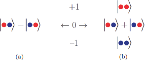
If we consider two waves, Ψ(A)_i that A located at i and Ψ(B)_j that B located at j, we consider (number of possible A) × (number of possible B) wave functions. If two kinds are available for both A and B, then there are four possibilities: Ψ(A₁)_iΨ(B₁)_j, Ψ(A₁)_iΨ(B₂)_j, Ψ(A₂)_iΨ(B₁)_j, and Ψ(A₂)_iΨ(B₂)_j, which are shown in Fig. 5. Here, the red and blue bullets denote two different wave functions. The first is the location i and the second is the location j. For a spin- wave, the eigenvalues are either or If one consider two spin- waves, the eigenvalues are either +1, 0 or −1. The four possible cases are split into Figs. 5(a) and 5(b). For the z-component spin value of 0, there are the antisymmetric (a) and symmetric (b) combinations. If the same position is considered, i = j, then the antisymmetric combination vanishes. The spin- electron wave of antisymmetric combination is excluded. This is the essence of the Pauli exclusion principle in filling up atomic energy levels. Pauli was the father of the spin-statistics theorem that the half-integer spin particles, the so-called fermions, satisfy the Fermi–Dirac statistics and the integer spin particles, the so-called bosons, satisfy the Bose–Einstein statistics. The Fermi–Dirac statistics chooses the antisymmetric combination and the Bose–Einstein statistics chooses the symmetric combination in Fig. 5. This spin-statistics theorem played an important role in finding quantum chromodynamics (QCDs) in the current atomic theory.

Figure 5: Product of two wave functions.

The relativistic formulation of quantum mechanics of electrons interacting with photons was written again by Paul Dirac in 1928, and is called quantum electrodynamics (QEDs). Since it describes the electron and photon waves, it is called quantum field theory of QED. Quantum fields (equal to waves supplemented by creation and annihilation operators satisfying Heisenberg’s uncertainty relation; thus quantum) also contain antiparticles, and in particular, Dirac predicted the antiparticle of electron, positron. In 1929, Dmitri Skobeltsyn detected positron that acted like electrons but curved in the opposite direction in an applied magnetic field.

Around this time, nuclear beta decay showed peculiar behaviour with the knowledge of the time. Beta decay was first observed by Henri Becquerel in uranium in 1896. Beta decays are the result of weak interactions as we know now; these are one of the main focus points probing modern atomic theory, but the story went through many hurdles. The first important idea was on the prediction of neutrino(s) by Wolfgang Pauli. James Chadwick observed the continuous energy spectrum of beta rays in 1914, which posed the problem “Why?”. At that time, nucleus, beta ray, and photon were the particles to be considered. In beta ray, photon is not considered. So, the continuous spectrum was a problem. There was an idea that the nuclear levels cascade down to lower states emitting photons, but in any case, there must be a primary electron which will kick out more electrons from outer shells of nucleus, which was not observed. Actually, it was puzzling enough that Niels Bohr suggested energy non-conservation only in beta decays. The nitrogen anomaly of that time was that ⁷N did not show Fermi statistics but Bose statistics (remember this time was before knowing the existence of neutron), i.e. Bose and Fermi statistics of nuclei at that time was determined by the charge number. In the nucleus model of that present, it was a dilemma and somehow Pauli knew the spin-statistics problem at that time. In 1929, Pauli was the Professor of Physics at the ETH Zurich, which might have been a centre of quantum mechanics then since people there then included Paul Dirac, Walter Heitler, Fritz London, Francis Wheeler Loomis, John von Neumann, John Slater, Leó Szilárd, Eugene Wigner, with Robert Oppenheimer and Isidor Rabi visiting there in March. At this time with his influential position, Pauli made the idea on neutrino public by writing a letter to the German Physical Society at Tübingen on December 4, 1930, “Dear Radioactive Ladies and Gentlemen, . . .“wrong” statistics of the N and ⁶Li nuclei and the continuous beta spectrum, I have hit upon a desperate remedy to save the exchange theorem of statistics and the laws of conservation of energy. Namely, the possibility that there could exist in the nuclei electrically neutral particles, that I wish to call neutrons,12 which have spin- and obey the exclusion principle . . . that neutron at rest is a magnetic dipole of a certain moment μ. The experiment seems to require that the effect of the ionisation of such a neutron cannot be larger than that of a gamma-ray and then μ should not be larger than e · 10⁻³ cm . . . it would have a penetrating power similar to, or about 10 times larger than, a γ-ray.” Obviously, he introduced an interaction¹³ responsible for the decay by μ, the magnetic moment interaction. But, Pauli’s number is 10⁸ times the Bohr magneton which translates to 10¹⁶ times larger rate if the Bohr magneton were used. Anyway, he considered his particle heavy, not the light one that we consider now.

Pauli’s neutrino was observed in 1956, 36 years after Pauli suggested, by Frederick Reines and Clyde Cowan, working in Hanford and Savannah River Sites. Reines and Cowan developed the equipment and procedures with which they first detected the supposedly undetectable neutrinos on June 14, 1956, by placing a detector within a large antineutrino flux from a nearby nuclear reactor. Now, it is known that there are three neutrino species: the electron-type ν_e, the muon-type ν_μ, and the tau-type ν_τ. These neutrinos transform to each other via the process known as neutrino oscillation. Unlike electron, muon, tau, and other coloured particles in Fig. 5 of Chapter 6, neutrinos are just two-component waves, the half of the others.

For 15 years between 1930 and 1945, there was not much theoretical progress. But here we note a very important discovery: the identification of another nucleon neutron by James Chadwick (1891–1974) in 1932, which guided the route to our current understanding of nucleus. Chadwick worked under Hans Geiger (1882–1945) several years since 1913. Acquainting with new technologies first is a guaranteed step towards new discoveries. The Geiger counter in 1913 provided more accuracy than earlier photographic techniques. In 1914, using the Geiger counter, Chadwick was able to demonstrate that beta radiation produced a continuous spectrum, as mentioned before, which led to Pauli’s suggestion of neutrino. At the time around 1925 when spin was already known, it was believed that the nucleus core consisted of protons and electrons. So, nitrogen’s nucleus with a mass number of 14 was assumed to contain 14 protons and 7 electrons. This gave it the right mass and charge, but the wrong spin (14 + 7 = 21 = odd number) as mentioned above by Pauli (note that neutron was not counted at that time and hence only the atomic number mattered).

Acquaintance with Geiger enabled Chadwick knew a better detector early enough in this period. In 1928, he was introduced to the more powerful Geiger–Miller counter. Because of the problems in beta decays, Chadwick and Ernest Rutherford (1871–1937) had been hypothesising a theoretical nuclear particle with no electric charge (the neutron) for years.14 If 7 “neutrons” are in the nitrogen nucleus in addition to 7 protons, the mass and charge of the nitrogen nucleus are explained. Then, the spin of the nitrogen nucleus would be even and the spin-statistics problem is satisfied. The major drawback with the earlier Geiger counter was that it detected alpha, beta and gamma radiation. The Cavendish laboratory where Chadwick and Rutherford worked in 1928 normally used the earlier Geiger counter in its experiments with radium. Radium emitted all three and was therefore unsuitable for what Chadwick had in mind for a theoretical nuclear particle with no electric charge. Polonium is an alpha emitter, and Lise Meitner sent Chadwick about 2 millicuries (about 0.5 g) from Germany.

In January 1932, Frédéric and Irène Joliot-Curie had succeeded in knocking protons from paraffin wax using polonium and beryllium as a source for what they thought was gamma radiation emitter. Rutherford and Chadwick disagreed; protons were too heavy for gamma radiation to push out (earlier, we commented that the heavy mass is needed for the collision effect to be large). But their theoretical nuclear particles with no electric charge would need only a small amount of energy to achieve the same effect. In Rome, Ettore Majorana came to the same conclusion. In retrospect, Frédéric and Irène Joliot-Curie had discovered the neutron, but did not know it. This reminds us that even experimentalists must have enough common sense on theoretical ideas.

To Chadwick, this was evidence of something that he and Rutherford had been hypothesising for years. Chadwick dropped all his other responsibilities to concentrate on proving the existence of the neutron. He devised a cylinder containing a polonium source and beryllium target and the suitable detection apparatus. In February 1932, after only about two weeks of experimentation, Chadwick confirmed his idea and sent the paper to Nature with the title “Possible Existence of a Neutron”. This was a rough sketch of how neutron was discovered and revolutionalised nuclear physics, and we remember Rutherford the father of nuclear physics and Chadwick the discoverer of neutron.

In 1933, Chadwick and Goldhaber showed by experiment that the neutron is slightly more massive than the proton which is an important fact for various reasons, e.g. it enables the weak interaction β-decay of a neutron into a proton.

In 1934, Fermi proposed his theory of beta decay which explained that the electrons emitted from the nucleus were essentially by the decay of a neutron into a proton, an electron, and an antineutrino. Fermi’s weak interaction Hamiltonian contained effectively 34 terms. On December 17, 1938, German Otto Hahn (1879–1968) and Fritz Strassmann (1902–1980) found the nuclear fission and nuclear reaction: A heavy nucleus spontaneously or by collision by a neutron split into two lighter nuclei. Nuclear reaction of a heavy nucleus, e.g. uranium 235, was used in early engineered nuclear devices. The available energy, enormous energy compared to energy from chemical reactions, was used in atomic bomb and later in nuclear reactors, currently supplying substantial portion of electric power in France, Japan, Korea, etc. One class of nuclear weapon, a fission bomb or atomic bomb, is a fission reactor designed to liberate as much energy as possible and as rapidly as possible.

Ettore Majorana (1906–1938?), mentioned above, disappeared very mysteriously. Nobody has seen him after he took off Palermo by ship to Naples on March 25, 1938. Since 1963, Italians commemorate him hosting schools in Erice (near Palermo), Sicily, mainly organized by high-energy experimentalist Antonino Zichichi (1929–), and in the booming period of gauge theories, important lectures were given in Erice.

But, his name is mostly cited these days on the nature of neutrinos. A massless neutral two-component spin- particle is called either a Weyl or a Majorana particle. If exactly massless, it does not matter which name we use. But, if it is massive, they are physically different.

Pauli considered two spin states of Fig. 3 and put the two states as a 2 × 1 column matrix and called it spinor. Then, the spinor wave function has two complex components and is called a doublet 2 in group theory. The non-relativistic Schrödinger equation satisfied by Ψ₂ is the Pauli–Schrödinger equation. Dirac generalized it to a relativistic form by combining with another spinor, effectively including the antiparticle. The non-vanishing mass makes all the four complex components be used. But, if mass is zero, consideration of two complex components is enough.

Out of the four complex components, there are two possibilities for reducing them to half, among which Majorana chose the case that the four complex components are reduced to half just by considering the four real comonents. The Dirac equation satisfied by the four real components is the Majorana equation satisfied by a Majorana particle. Choosing just the reality condition allows non-zero mass for a Majorana particle. The other way, reducing the four complex components to two complex components, gives the ‘Weyl’ spinor which cannot be realized if mass is non-zero. To make up mass by Weyl spinors, two Weyl spinors are needed. Since neutrino masses are known to be non-zero, it is important to check whether they are of Majorana type or Dirac type.

Hideki Yukawa (1907–1981) was a Japanese theoretical physicist and the first Japanese Nobel laureate known for his prediction of the pi meson. After receiving his degree from Kyoto Imperial University in 1929, he stayed there as a lecturer for 4 years and then moved to Osaka Imperial University as Assistant Professor. There, he proposed the pion as the mediator of the nuclear forces. In 1940, he won the Imperial Prize of the Japan Academy, and in 1949, he was awarded the Nobel Prize in Physics after the discovery of pions by Cecil Frank Powell, H. Muirhead, Giuseppe Occhialini and Céesar Lattes of Yukawa’s predicted charged and neutral pi mesons (π^±, π⁰) in 1947. The masses of these pi mesons are (139.6 MeV, 135.0 MeV).

In 1935, Yukawa published his theory of mesons in the Proceedings of Japanese Mathematical Society,15 considering a charged scalar particle (with a fortunate sign mistake). He showed that its mass must be about 200 times electron mass, which was a major influence on the research into elementary particles. Yukawa’s group at Osaka, including Sakata, Taketani, and Fushimi, intensively developed the theory of mesons. Yukawa argued that there must be not only charged bosons but also neutral boson. In 1937–1938, he believed that vector bosons are better than scalar bosons to explain spectrum and properties of nuclei. According to Yutaka Hosotani, the neutral pseudoscalar pion was realized much later.

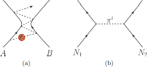
Yukawa’s meson potential is the beginning of the study of forces by exchanges of integer-spin particles. It is like considering two figure-skate players exchanging a basketball as they skate, as shown in Fig. 6(a). When the skater A tosses the basketball, his trajectory shifts a bit to compensate the momentum carried by the basketball, satisfying the momentum conservation. When the skater B receives and tosses back the ball, his trajectory shifts a bit by the same argument. Continuous exchanges of the ball ends up hyperbolic trajectories of both skaters A and B. Observers looking at A’s and B’s trajectories would consider that there is a repulsive force between them. Yukawa mimiced this repulsive force by introducing unnoticeable mediator basketball in this case. In the modern jargon, the mediator is an elementary particle pion, which is depicted as the propagator in the Feynman diagram in Fig. 6(b).

The force law obtained in this way is exponentially suppressed related to the mass of exchanging particle. Because nuclear forces in the nucleus do not extend beyond the nuclear size, Yukawa predicted the mass of pion to be around 200 times the electron mass. If the mass of the exchanged particle is heavy, the trajectory is more curved compared to a light particle exchange. One can understand that exchange of a ping-pong ball may not affect the curving of the trajectory very much. The same happens in the world of atoms. If a low-energy photon is exchanged, the trajectories are almost in the forward direction. In this sense, the UA1/UA2 experiments of 1982 in discovering Z⁰ and W ^± bosons and the recent LHC experiments looked for hard collision events to find heavy particles.

Figure 6: An idea of Yukawa’s pion.

But, the above explanation misses one important fact. Figure 6(a) describes a replusive force while we need an attractive force for binding protons and neutrons strongly inside a nucleus. So, it is better for A and B to be connected by a rope. From time to time, A and B attract the rope such that they come closer. The oscillation of the rope may be considered as a wave describing the exchanged particle. More technically, exchange of a spin-0 particle always gives an attractive force. For spin-1 particle, such as photon, it can give repulsive or attractive force, depending on the relative charges of the two particles. Furthermore, in a more technical jargon, the spin-0 particle appearing in relation to the unitary group is always “pseudoscalar”. So, what Yukawa predicted was a pseudoscalar triplet, π^±, π⁰, a representation of the unitary group SU(2).

As in many other cases, this intermediate particle idea was also considered by another physicist. It was by Swiss mathematician and physicist, Baron Ernst Carl Gerlach Stückelberg von Breidenbach zu Breidenstein und Melsbac (1905–1984), who is regarded as one of the most eminent physicists of the 20th century. Stückelberg’s sojourn in Zurich in 1932 led to contact with leading quantum theorists Wolfgang Pauli and Gregor Wentzel, which in turn led him to focus on the emerging theory of elementary particles. Stückelberg’s intermediary was a massive spin-1 particle, and he discussed his idea with Wolfgan Pauli who immediately rejected the idea. When we assess why Pauli objected to Stückelberg’s idea immediately, we note that it is because Pauli was the guru understanding gauge forces. With spin-1 particle exchange, big nucleus is full of repulsive protons, and hence, he might not have agreed to Stückelberg’s idea.

Yukawa’s original idea was exactly like Stückelberg’s spin-1. But, Yukawa was lucky. He submitted the idea to Physical Review, for which Robert Oppenheimer was the Editor at that time. Oppenheimer considered it being submitted from a backward country not knowing physics (at that time) and rejected it outright.16 So, Yukawa’s wrong idea was not published. Nevertheless, he continued with pseudoscalar intermediary, which we call pions now. Six months after rejecting Yukawa’s wrong idea, Oppenheimer considered that Yukawa’s idea was not that bad actually and felt sorry for his rejection for a long time. This might be one reason that he recommended Yukawa to the Nobel Committee in 1949.

In 1936, right after Yukawa’s suggestion of pions, Carl Anderson (1895–1991) and Seth Neddermeyer (1907–1988) at Caltech observed particles heavier than electron and lighter than proton from cosmic rays.¹⁷ They noted particles that curved differently from electrons and were negatively charged but curved less sharply than electrons, but more sharply than protons. Thus, Anderson initially called the new particle a mesotron, adopting the prefix meso- from the Greek word for “mid-”.¹⁸ Initially, it was considered as the pion that Yukawa suggested, just from the mass region. But, the single long track did not look like a strongly interacting pion. The existence of this deeply penetrating particle was confirmed in 1937 by J. C. Street and E. C. Stevenson’s cloud chamber experiment.¹⁹ Now, it is called muon.

Before the end of WWII, only photon, electron and muon were discovered among the fundamental particles of the Standard Model shown in Fig. 5 of Chapter 6.

1Michael D. Gordin, A Well-ordered Thing: Dmitrii Mendeleev and the Shadow of the Periodic Table (Basic Books, 2004), pp. 229–230; ISBN 978-0-465-02775-0.

²B. M. Kedrov, On the Question of the Psychology of Scientific Creativity (On the Occasion of the Discovery by D. I. Mendeleev of the Periodic Law), A Journal of Translations, VIII(2), 18–37 (1967), translated by H. A. Simon (Carnegie Institute of Technology) from [Voprosy psikhologii, 3(6), 91–113 (1957)].

³A. Karpov, Synthesis of superheavy elements: Present and future, Talk presented at the 19th Lomonosov Conference on Elementary Particle Physics, Moscow State University, August 22–28, 2019.

⁴J. W. Moore; C. L. Stanitski and P. C. Jurs, Chemistry: The Molecular Science, Volume 1 (Brooks/Cole, 2014); ISBN-13: 978-1285199047.

⁵J. C. Maxwell, On Physical Lines of Forces, Philosophical Magazine & Journal of Science, March (1861).

⁶J. C. Maxwell, A Dynamical Theory of the Electromagnetic Fields, Philosophical Transactions of the Royal Society of London 155, 459–512 (1865).

⁷S. Weinberg, Dreams of a Final Theory (Vintage Books, Random House, New York, 1994).

⁸Susumu Okubo’s comment to the second author at Rochester, New York, January, 2010.

⁹There is another number under the name of Planck mass: M_P = 2.43 × 10¹⁸ GeV.

¹⁰B. Green, The Elegant Universe (W. W. Norton, USA, 2003) and C. Rovelli, Reality is Not What it Seems (in English) (Penguin Group, New York, 2016).

¹¹G. Farmelo, The Strangest Man: The Hidden Life of Paul Dirac, The Mystic of Atom, (Basic Books, New York, 2009). The words on his gravestone are “. . . because God made in that way. . ..”

¹²After neutron was discovered, Pauli’s particle was called neutrino.

¹³It was the time before Fermi’s writing of the weak interaction Hamiltonian.

¹⁴A. Brown, The Neutron and the Bomb: A Biography of Sir James Chadwick (Oxford University Press, 1997); ISBN 978-0-19-853992-6.

¹⁵H. Yukawa, On the Interactions of Elementary Particles I, Proceedings of Japanese Mathematical Society 17, 48–57 (1935) [Progress of Theoretical Physics Supplements 1, 1–10 (1955) [doi.org/10.1143/PTPS.1.1]].

¹⁶Susumu Okubo’s comment to the second author at Rochester, New York, January, 2010.

¹⁷C. D. Anderson and S. Neddermeyer, New Evidence for the Existence of a Particle of Mass Intermediate Between the Proton and Electron, Physical Review 52, 1003 (1937).

¹⁸This prefix transferred to Yukawa’s pions. Now, mesons mean strongly interacting bosons, including pions and other bosons made of a quark and an antiquark.

¹⁹J. Street and E. Stevenson, New Evidence for the Existence of a Particle of Mass Intermediate Between the Proton and Electron, Physical Review 52, 1003 (1937).