Chapter 6

Particle Theory

In 1942, the wartime Manhattan Project gathered the US talents in nuclear physics at Los Alamos, New Mexico. The project, led by Major General Leslie Groves (1896–1970) and theoretical physicist Robert Oppenheimer (1904–1967), succeeded in making the atomic bomb which was tested in the New Mexico Desert at 5:30 a.m. on July 16, 1945 with an energy equivalent of around 20 kilotons of TNT, having left a crater called Trinitite. Many nuclear physicists who participated in the Manhattan Project opened the field of particle physics or high energy physics.

After WWII, Oppenheimer joined The Institute for Advanced Study at Princeton as the director. He convened 25 leading physicists at Ram’s Head Inn on Shelter Island near the tip of Long Island, New York, for a one-day conference on June 1, 1947. Some participants were Willis Lamb, Richard Feynman, Julian Schwinger, Hans Bethe, Enrico Fermi, and Robert Marshak. The main topic of interest at this conference was the observation of the Lamb shift. At this time, the accepted particle theory was quantum electrodynamics (QED), formulated by Paul Dirac in 1928. But, these talented physicists could not explain the Lamb shift.

Oppenheimer’s conference continued at Pocono Manor, Pocono Mountains, Pennsylvania, in 1948 and at Oldstone-on-Hudson near New York in 1949. From the beginning of this series, the infinity first encountered in the explanation of the Lamb shift was the hurdle to be overcome. In the 1948 meeting, Schwinger presented a largely completed work, and Feynman’s exposition known as Feynman diagrams (largely orchestrated by Oppenheimer) was presented at the 1949 meeting. By this time, QED was able to present refined calculations of electron interactions mediated by photons. So, Oppenheimer achieved his goal of understanding the original infinities in QED and finished his conferences.

Robert Oppenheimer was known to be a philanthropist, a genius, and a poet as noticed from comments after his death: the Times of London described him as the quintessential “Renaissance man”, and his friend David Lilienthal told the New York Times, “The world has lost a noble spirit — a genius who brought together poetry and science.” Also, in 1963 on the occasion of Fermi Prize award, CBS broadcaster Eric Sevareid described him as “the scientist who writes like a poet and speaks like a prophet.” He died on February 18, 1967, and the urn of his ashes was lowered into Hawksnest Bay, St. John, Virgin Island. He opened the window toward modern-day atomic theory.

By 1949, as mentioned above, interactions between electrons and photons were completely understood in terms of QED. The calculation of the magnetic moment of electron in QED is 1.001 159 652 181 64 (±76), while the observed value is 1.001 159 652 180 91 (±26). So, the QED accuracy is correct up to 1 part in 1,000,000,000,000, and is the most successful scientific theory. Since 1949, numerous strongly interacting particles had been observed. The well-known one is the pion mentioned earlier. This pion and the related strong interaction were not understood in 1949. It was a problem to understand pions and related particles.

For the purpose of understanding pions and other strongly interacting particles, the first Rochester Conference was organised by Robert Marshak, then Chairman of Physics at the University of Rochester, and held on December 16, 1950. The next several Rochester Conferences witnessed the cradle of particle physics: discussions on the tau–theta puzzle, parity violation, and the so-called “V–A” theory in weak interactions. In the session presided by Oppenheimer on “Theoretical Interpretatioin of New Particles” on the last day of Rochester-6 (1956),1 the puzzle related to the tau and theta particles was the main topic. After Chen Ning Yang’s talk, Feynman brought up a question of Block’s, “Could it be that the tau and theta are different parity states of the same particle which has no definite parity, i.e. parity is not conserved?”

During ICHEP-6, Feynman shared a room with Martin Block (1925–2016), and one evening Block said to Feynman, as was written in Surely You Are Joking,² “Why are you guys so insistent on this parity rule? Maybe the tau and theta are the same particle. What would be the consequences if the parity rules were wrong?”

The solution of the tau–theta puzzle was that weak interactions, in the nuclear beta decays, in hyperon decays, and in the decays of mesons, in general do not respect the space inversion symmetry, called the “parity” operation. In late 1956, the parity violation in weak interactions was suggested by Tsung Dao Lee (1926–) and Chen Ning Yang (1922–). Parity violation is the unique feature in the weak force among the four known forces: electromagnetic, weak, strong, and gravitational forces. The Lee and Yang paper raised the important experimental question of whether weak interactions were parity invariant, meaning that they would be the same if the experiment were reflected in a mirror. Yang has told the first author that they did not expect parity to be violated, and indeed Lee and Yang changed their research interest to statistical mechanics. Nevertheless, they were surprised and delighted when the experiment of Madame Chien-Shiung Wu (1912–1997) and collaborators showed that parity was maximally violated in weak interactions. The experiment involved studying the β-decay of polarised Cobalt-60 nuclei, as suggested to Lee and Yang by Maurice Goldhaber (1911–2011). This result was a surprise to most physicists and did lead to the award of a Nobel Prize immediately in 1957. The parity violation in weak interactions opened a new field: particle physics. Before 1957, there was no word “particle physics”.

After 1957, particle physicists differentiated from the study of nuclear physics, looking for much shorter distance scales compared to the nuclear size, i.e. paying much more attention to higher energy scales. This is the reason particle physics is synonymous with high-energy physics (HEP), and the international conference of particle physics is called ICHEP.

After it was accepted that parity is violated in the charged current (CC) weak interactions, Rochester-7 was short of announcing the “V–A” theory of CC weak interactions. There is an anecdote at Rochester-7 that George Sudarshan, a graduate student at Rochester, asked Robert Marshak to present their recently completed idea of “V–A” theory of weak interactions. But, Marshak as the chairman of the LOC did not allow his talk, replying that Martin Block was supposed to mention their work. But, Block did not appear, so Marshak presented their work at the Padova conference four months later. Between Rochester-7 and 8, it was advocated by Marshak, Sudarshan, Feynman, and Gell-Mann that the CC weak interactions chose only the “V–A” part but never “V+A”. These four famous physicists are the “V–A” quartet. From this time on, only one coupling constant G_F has been used for all the CC weak interactions out of Enrico Fermi’s 34 constants, and developments in particle physics have been possible from this time on, finding symmetries required for understanding weak and strong interactions at the level of QED. This “V–A” theory was the cornerstone to the road to the Standard Model (SM) and Shoichi Sakata’s symmetry was the beginning in the search for strong interaction symmetries. However, there is one more hurdle to be overcome, which is discussed in more detail in Chapter 7.

The year 1964 was a creative year. Then, Gell-Mann’s mathematical quark (or Zweig’s Ace) loomed in his cherished eight-fold way of currents, the weak CP violation was observed by the Princeton group, and the Brout–Englert–Higgs–Guralnik–Hagen–Kibble (BEHGHK) mechanism, the Higgs mechanism in short, was known. A year later in 1965, an additional SU(3) degree (later known as colour) for strong interactions was proposed by Moo-Young Han and Yoichiro Nambu. Gell-Mann’s mathematical quark and colour SU(3) were accepted ten years later at the November Revolution of 1974. The BEHGHK mechanism was finally proved by the discovery of the 125 GeV boson in 2012. For the weak CP violation phenomena, it was in 2006 that three families of quarks in the SM were considered enough to explain them all. During this crucial period, the ICHEP-12 was held in a small town Dubna, on the banks of Volga River, USSR (August 5–12, 1964). Val Fitch (1923–2015) brought and showed his Princeton apparatus, which had discovered the weak CP violation. It was a period when tabletop experiments could reveal important aspects of particle interactions.

The BEHGHK mechanism was known in 1964, but even in the ICHEP-13 Berkeley in 1966, plenary sessions did not include spontaneous symmetry breaking. The year 1967 was the year for this to get attention3 in the conference (with 325 theorists participating) dedicated to the late Robert Oppenheimer, who passed away on February 18, 1967, which is considered to be the commencement year of the SM by representing the quark and lepton doublets only in the left-handed sector by Steven Weinberg, realising the “V–A” nature of the weak CC formulated in 1957 by “V–A” quartet. But, the SM needed a few more years to bloom until the renormalisability of the spontaneously broken gauge theories was proven in 1971 by Gerard ’t Hooft (1946–) and Martinus Veltman (1931–). The ICHEP series expanded since the ICHEP-16 Chicago, which was held at Fermilab during September 6–13, 1972, with the number of participants exceeding 300.

As mentioned in the end of Chapter 5, there were two similar particles known before the end of WWII: electron and muon. Muons behaved exactly the same way as electrons in QED and weak interactions except for their mass difference. This repetition problem was succinctly expressed as “Who ordered that?” by Isidor Issac Rabi (1898–1988) of Columbia University in 1937 in response to the news that the 1936-discovered muon was not a hadron but a new and entirely unexpected type of lepton. Still, this was the culminating phrase on the current flavour problem or the family problem. The question on the difference of electron and muon masses was one of the flavour problems. It is said that in the United States of America, Oppenheimer was the first theoretician and Rabi was the first experimentalist understanding quantum mechanics. Rabi and Oppenheimer were good friends since 1929, as mentioned earlier, and went to Zürich together, and maintained their friendship through their lifetime during the Manhattan Project years and afterward also. Another Rabi quip is “We have an A-bomb and a whole series of it, and what do you want, mermaids?” to the Atomic Energy Commission, defending Oppenheimer against charges of leaking classified information during the McCarthyism era.4

A legacy of the Manhattan Project led by Oppenheimer was the network of researchers in the United States, but no national laboratory comparable to the one at Los Alamos was located on the East Coast of the United States. Isidor Rabi and Norman Ramsey, both at Columbia University, assembled a group of universities in the New York area to lobby for their own national laboratory. Rabi had discussions with Major General Leslie Groves, whom he knew from the Manhattan Project, who was willing to go along with a new national laboratory. Moreover, while the Manhattan Project still had funds, the wartime organisation was expected to be phased out when a new authority came into existence. After some discussions, the two groups agreed in January 1946. Finally, nine universities (Columbia, Princeton, Rochester, Pennsylvania, Harvard, Cornell, MIT, Yale, and Johns Hopkins) came together, and on January 31, 1947, a contract was signed with the Atomic Energy Commission (AEC), which had replaced the Manhattan Project, that established the Brookhaven National Laboratory(BNL).5 After establishing the BNL, Rabi suggested to Edoardo Amaldi (1908–1989) that BNL might be a model which Europeans could benchmark. Rabi saw science as a way of inspiring and uniting a Europe that was still recovering from the war. An opportunity came in 1950 when he was named the United States Delegate to the United Nations Educational, Scientific and Cultural Organization (UNESCO). At a UNESCO meeting at the Palazzo Vecchio in Florence in June 1950, he called for the establishment of regional laboratories. These efforts bore fruit; in 1952, representatives of eleven countries came together to create the Conseil Européen pour la Recherche Nucléaire (CERN). Rabi received a letter from Bohr, Heisenberg, Amaldi, and others congratulating him on the success of his efforts. Now, the bronze sculpture of Niels Bohr’s face is displayed at the CERN Library. The Higgs boson in Fig. 5 was discovered at the LHC of CERN.

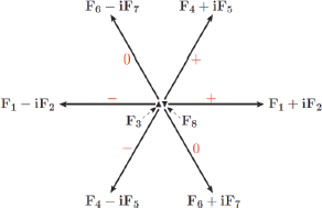
In 1963, one important flavour regularity on hadrons was observed by Italian physicist Nicola Cabibbo (1935–2010). He was considering decay rates triggered by the charged current (CC) weak interactions. A family of 15 chiral fields, which are mentioned at the end of this chapter, consists of three chiral leptons and twelve chiral quarks. Decays of particles such as the beta decay are going through the CC weak interactions. If there was only one family, there is only the decay of neutron and pion by the CC interaction. If there are two families, we can consider additional possibilities due to the addition of the second family, i.e. the decays of muon (μ) and strange(s)/charm(c) particles as shown in Fig. 5. In 1963, charmed particles were not known. So, he compared rates of the muon decay, the beta or neutron decay, and the Lambda (= a strange baryon) decay, obtaining (muon decay rate) = (neutron decay rate) + (Lambda decay rate) after factoring out kinematic factors properly. If one squared value is the sum of two squared values, then it is the Pythagoras theorem for a right triangle, i.e. 1 = cos² θ + sin² θ. We call this angle observed in the above CC weak interaction the Cabibbo mixing angle θ_C, which is about 13°. When we say an angle, it appears naturally in some unitary transformation as mentioned before. Therefore, it is a quantum mechanical effect because two wave functions are mixed. In classical mechanics, one never considers mixing of two particles. The Cabibbo angle is for the case of mixing two waves, i.e., those of neutron and Lambda. In the quark model, it describes a mixing angle of d and s quarks. In 1963, the quark model was not known. But, the eight-fold way of currents in strong interactions shown in Fig. 1 was known chiefly by Murray Gell-Mann. Among these, the plus CCs are (I₊ ≡ F₁ + iF₂) and (V₊ ≡ F₄ + iF₅). So, quantum mechanics allows a unitary transformation, with the absolute magnitude 1 such that these two combinations are mixed. This combination appearing in e^iFCθC is describing both beta decay and Lambda decay. On the contrary, the muon decay does not belong to the eight-fold way since there is no strongly interacting particle involved. Therefore, the corresponding unitary transformation is just a phase multiplication. Relation between these is basically 1 = cos² θ_C + sin² θ_C. This was the reason that Cabibbo found the unitary transformation even before the advent of the quark model. In fact, Gell-Mann and Lévy included a footnote in their σ-model paper published in 1960 in the Italian journal Nuovo Cimento, “Of course, what really counts is the nature of the commutation relations for the complete operators that generate the sum of the ΔS = 0 and ΔS = 1 currents,” where S is the strangeness quantum number of hadrons. We may understand their “complete operators” as our one unitary operator, but it is not clear what they meant by complete. Gell-Mann and Lévy were to Cabibbo what Greek atomists were to Dalton, based on the accounts of the observed facts. After the quark model was proposed, this mixing effect is written as Cabibbo’s mixed quark, mixing between the d quark and the s quark: d′ = d cos θ_C + s sin θ_C.

Figure 1: Eight-fold way of currents.

In the eight-fold way in Fig. 1, there are four neutral currents, corresponding to F₃, F₈, F_6+i7, and F_6−i7. A magnitude 1 unitary transformation can be a combination of these four, but here F_6±i7 does not conserve the strangeness quantum number. At the weak interaction level with the Fermi constant G_F, the strangeness changing neutral current (SCNC) effects were not observed until 1970. So, there was a need to remove this SCNC. The answer was provided by Sheldon Glashow, John Iliopoulos, and Luciano Maiani (GIM) in 1970 by introducing an additional quark charm c, and by introducing another mixing between the d and s quarks: s′ = −d sin θ_C + s cos θ_C. It is said that Ziro Maki and Yoshio Ohnuki introduced the fourth quark c in 1964, but Maki and Ohnuki are to GIM what Greek atomists are to Dalton.

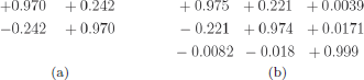
Earlier, we mentioned two mixing relations with one angle, d′ and s′. This case is succinctly written by four numbers to generate the unitary matrix of mixing d and s quarks in terms of one angle. The Cabibbo angle of 13 degrees, to make a unitary matrix, is implied by displaying a set of four numbers as shown in Fig. 2(a). If three quarks mix, we need three angles to discuss the quantum mechanical mixing of three quarks. In this case, we need an array of nine numbers as shown in Fig. 2(b). The SM has six quarks and we need mixing between only half of these quarks, i.e. d, s, and b quarks or u, c, and t quarks. Theoretically, not only the gauge interactions, as discussed above in terms of currents, but also the particle masses participate in physics of elementary particles, for example the Higgs boson interaction with quarks to render quarks massive. In sum, physics related to inter-family relations is called the family problem or the flavour problem.

Figure 2: Arrays of numbers.

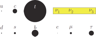
Figure 3: Relative sizes of masses. The masses of neutrinos are so small compared to the electron mass, at least a hundred-millionth, their sizes cannot be shown in the figure. In the yellow band, it is only shown that there are three small masses.

The masses of quarks and leptons are schematically shown in Fig. 3. We notice that there is a hierarchy of masses of order hundred million between the electron and top quark. As noticed from Figs. 2 and 3, this flavour problem in the quark sector is a very difficult problem. So far, we looked for how Nature revealed its secret regularities to us but Figs. 2 and 3 seem to not hint at any simple regularity. The flavour problem is considered the most important remaining theoretical problem in the SM.

In the leptonic sector also, there are mixings. Since we already know that there are three families, let us discuss the mixing of three lepton families. Generalisation of the strangeness changing neutral current is the flavour⁶ changing neutral current(FCNC). The absence of FCNC at order G_F in the leptonic sector is also verified from the negligible rate for muon to electron plus photon, μ → e + γ, in the decay of muon. Since the flavour problem brings in the masses of each particle, the mass generating mechanism is important in the flavour problem or in understanding the observed number of arrays shown in Fig. 2. According to Einstein, mass is energy as known by his famous formula E = mc². Therefore, mixing must be considered with the energies under consideration: the kinetic energy and potential energy. At low energy, mass belongs to the potential energy. In the quark sector, the kinetic energies in the experiments we chose are much smaller, and the fact that mixing depending on mass is all we need to consider.

In the leptonic sector, let us choose masses such that Q_em = −e leptons are already diagonalised. And, we discuss three neutrinos of Fig. 3 without worrying about diagonalisation of charged leptons. The kinetic energies of the observed neutrinos vary over a wide range. Reines and Cowan’s nuclear reactor electron antineutrinos are several MeVs. Lederman, Schwartz, and Steinberger’s muon neutrinos from Alternating Gradient Synchrotron of BNL are 200 MeVs. Neutrinos for the T2K (Tokai to Kamioka) experiments used for the observation of the tau neutrinos are from the 50 GeV proton source at J-Park, Japan. All these kinetic energies are much larger than any mass of three neutrinos. So, the neutrino mixing, or the flavour mixing in the leptonic sector, is observed by the mixing effects in the kinetic energy of neutrinos. The kinetic energies are compared to the differences of neutrino mass energy. Calculations show that leading mixing effects (or neutrino oscillation) occur at the difference of squared neutrino masses Δm². In the mixing, we have angles which are dimensionless since they are arguments in the phase, and hence Δm² appears in the numerator in the phase since more mass difference gives faster oscillation. Therefore, we expect a dimensionless argument Δm² × (distance travelled by neutrino)/(kinetic energy). This formula was first obtained by Russian physicist Bruno Pontecorvo in 1957 for the case of electron-type neutrino and antineutrino oscillation. Note that only the electron-type neutrino was known in 1956, and hence Pontecorvo considered the ν_e and oscillation.

Oscillations of three neutrinos require three real angles by an array of the type shown in Fig. 2(b), but the leptonic sector gives a different set of numbers from the shape for the numbers corresponding to quarks. Since neutrino oscillation experiments depend on the distance travelled by neutrinos, there are short baseline experiments, long baseline experiments, and even the very long distance for Solar neutrinos. Two of the three vertical numbers of Fig. 2(b) were first obtained from cosmic ray neutrinos scattering with nuclei in the atmosphere. Short baseline experiments looking for relatively large differences of squared masses are done by placing detectors near nuclear reactors. The Raymond Davies (1914–2006) Solar neutrino problem was that he did not see as much electron neutrinos as calculated by theorists, notably by John Bahcall (1934–2005), through the nuclear fusion processes in the core of the Sun. On the contrary, long baseline experiments can see the effects of very small squared mass differences, enabling one to observe the CP violation better. Now, we discuss the CP violation observed in the quark and leptonic sectors.

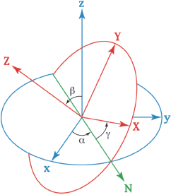
We discussed three angles to represent mixing between three particles. These angles are called Euler angles, introduced by Leonhard Euler (1707–1783), to describe the relative orientation of two rigid bodies of the same shape. As shown in Fig. 4 where the centre of weight is at the origin, first rotate the solid around the axis z by an angle α, then around the axis N by an angle β, and finally around the axis Z by an angle γ. The angles α, β, and γ are called three Euler angles.

Figure 4: Proper Euler angles drawn by Lionel Brits in Wikipedia.

Mixing in terms of only real angles cannot describe the CP violation. Here, C is the transformation of a particle to an antiparticle such as changing an electron to a positron. P is the inversion of spatial coordinates. If x denotes the three coordinates of a particle, change its position to −x: it is parity P. The combined operation, changing a particle to its antiparticle with the inverted coordinates, is the CP transformation on the particle. Forces or interactions acting on paricles are the roles of spin-1 particles in the second annulus in Fig. 5. There is no confusion describing photon as a real particle. Quantum mechanical transformation is a unitary transformation, and hence a photon does not change to another by C. For that matter, gluons behave in the same way. So, gluons also respect C. For the inversion of coordinates, it is known in the history of QED since 1928 that it respects P. The effect of neutral currents is flavour conserving and we do not pay attention to the interactions resulting from Z of Fig. 5, without worries about the FCNC effects. Gluons behave in the same way as QED at the tree level.⁷ There remain the effects of W^± interactions, i.e. those of CCs of matter fermions. Since CCs are defined only for the triangled fermions in Fig. 5, C and P are violated and there is no argument at this stage against CP violation in the CC weak interaction. If antiparticles behave exactly in the same way with the real number set of Fig. 2(b), then there is no way to decide whether we are looking at particles or antiparticles. To have a difference in the particle and antiparticle interactions due to W^±, there must be an additional parameter. It must be a phase since the role of three Euler angles is completed by three real angles. A phase must appear in the array of Fig. 2(b). This possibility was found by Mokoto Kobayashi and Toshihide Maskawa in 1972. Namely, a phase e^iδ appears at some entries in Fig. 2(b). Similarly, if a phase appears in the leptonic number arrays, then there is the weak CP violation in the neutrino oscillation.

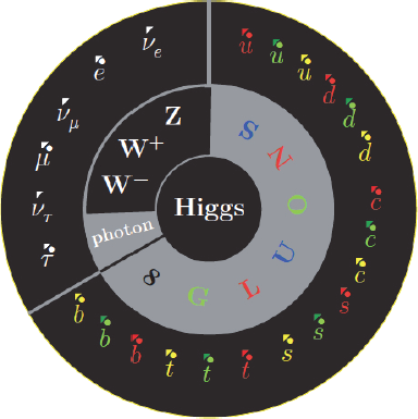
Figure 5: Particles in the SM. Particles on the grey disk are massless, and all the other particles obtain mass due to the Higgs boson. Quarks are repeated three times, which is symbolised by red, green, and yellow. White particles do not carry colour. Helicities are denoted by triangle for L-handed and bullet for R-handed. Neutrinos have only the L-handed helicity.

Let us list all the fundamental particles of the SM in Fig. 5. Any particle beyond those in Fig. 5 is a beyond-the-Standard-Model (BSM) particle. All particles of Fig. 5 are confirmed by particle physics experiments. After the hint that the SM might be correct, particle physicists looked for the effects of the SM particles outside the terrestial environment: in the cosmos and stars. Now, it is accepted that there are hints through dark matter and dark energy that the universe evolved with the effects of the BSM particles. However, these were not among the atomists’ view in the classical Greek period. Dark matter particles and sterile neutrinos are the BSM particles. In Fig. 5, massless particles are in the grey, which include photon and eight gluons. All the other particles are massive due to the Higgs mechanism. The force mediators are on the second annulus: gluons for the strong interaction, photon for the electromagnetic interaction, and W^± and Z for the weak interaction. The so-called matter particles, the Greeks’ dream, are on the outer annulus. The strongly interacting quarks come in three colours to act as charges of the gluonic force. Weakly interacting particles, not participating in the strong interaction, are leptons, which are shown as white. Here, helicities are denoted by a triangle for L-handed and a bullet for R-handed. Quarks and leptons possessing the same gauge force interactions repeat three times, for which we say, “There are three families in Nature.” At the centre, we placed the BEHGHK boson, simply called the Higgs boson whose mass is 125 GeV. Before considering “spontaneous symmetry breaking”, the complex Higgs doublet includes four real fields. After “spontaneous symmetry breaking”, among these four, three becomes the longitudinal degrees of W ^± and Z in the second annulus and the remaining real field is the 125 GeV Higgs boson. The BEHGHK mechanism is technically realised by assigning a vacuum expectation value (VEV) to one complex component of the doublet, say with the value V_EW. In one scheme, we have the SM scale where VEV is V_EW = 246 GeV.

Without many new fundamental discoveries between 1990 and 2012, theorists were free to think about BSM physics without much to worry about. During this period, observations into the sky revealed the need to understand dark matter (DM) and dark energy (DE) as much as atoms. Since the SM particles of Fig. 5 are short of explaining both DM and DE, one has to consider the BSM particles. When we consider these cosmologically hinted phenomena, the classical theory on gravitation must be considered as well. The minimal requirement is to study gravity only with the Einstein equation for gravitation. Regarding DE, Mordehai Milgrom (1946–) introduced an acceleration parameter a in gravity, ∼ 10⁻¹⁰ m/s², by naming it Modified Newtonian Dynamics (MOND), which was boosted by Jacob Bekenstein (1947–) (who is famous for suggesting the area rule for the black hole entropy). This acceleration parameter a allows for the distance dependence of gravitation force to deviate from the inverse square rule and gives the observed gravitational effects correctly for the nearby galaxies, but gives a difference for the Type-1 supernovae from which DE was suggested due to their acceleration.

The final words of this chapter are on the BSM-related theories: grand unified theories (GUTs), supersymmetry, supergravity, superstring, DM, DE, WIMPs, “invisible” axions, inflation, and extra dimensions.

“Why is the SM scale so small compared to the Planck mass, 2.43 × 10¹⁸ GeV”8 is the so-called gauge hierarchy problem in the SM. For fermions such as quarks and leptons, their masses can be neglected at the Planck mass if the L-helicity and R-helicity do not match properly. “Properly” means by considering all symmetries under consideration. The symmetry present in Fig. 5 is the SM gauge symmetry SU(3) × SU(2) × SU(1). For example, neutrinos in Fig. 5 arise only with L-handed helicity, which means that neutrino masses can be neglected at the Planck mass scale. It is said that neutrinos are chiral. All the other fermions in Fig. 5 are chiral also by considering the SM gauge group. These fermions lose the chiral property if the SM is spontaneously broken by the BEHGHK mechanism. At present, there is no universally accepted solution of the gauge hierarchy problem. Nevertheless, requiring a chiral property in a final theory is very plausible, as emphasised by Howard Georgi in 1979. Basically, this requirement was started since the “V–A” quartet of 1957 : Marshak, Sudarshan, Feynman, and Gell-Mann. When Feynman was asked what was his most important achievement,⁹ he replied, “the V–A model”.

Counting the number of triangles and bullets in Fig. 5, we have 3 × 3 for whites and 2 × 18 for reds, greens, and yellows, in total 45. It is said that 45 chiral fields are in the SM. Since there are three families, one family contains 15 chiral fields. In 1974, Howard Georgi and Sheldon Glashow grouped these 15 chiral fields into 5 and 10 to arrive at a unifying gauge group SU(5). Because neutrinos are known to be massive, sometimes it is useful to introduce R-handed counterparts of neutrinos. In this case, one family can be considered in terms of 16 chiral fields. With 16 chiral fields, a unifying gauge group SO(10) was considered by Howard Georgi, and also by Harald Fritzsch and Peter Minkowski in 1974–1975. Quarks and leptons are grouped with the same group property in these SU(5) and SO(10) groups. Hence, SU(5) and SO(10) were considered to be a true unification, and so they are called grand unification groups (GUTs). Still earlier in 1973, Jogesh Pati (1937–) and Abdus Salam (1926–1996) treated quarks and leptons in the same way, but the resulting group was not as simple as SU(5) and it is also called a GUT. Since quarks and leptons are treated in the same way as GUTs, it is possible to transform a proton made of three quarks to a lepton, i.e. a proton can be unstable in GUTs. Discovery of proton decay, though, is not convincing evidence of GUTs because it is possible to make a proton decay without a GUT, for example in an extension of the SM by supersymmetry.

As noticed above in relation to massless fermionic particles, viz., Fig. 5, the chirality concept is natural when we consider very small masses at the Planck mass scale or at the GUT scale. The well-known idea cited by people but not working within this program was the Kaluza–Klein (KK) idea on the electron mass. Naturally, the electron mass in the KK idea was at the Planck scale. This was corrected by Edward Witten in the second Shelter Island Conference in 1983. It was not worthwhile to spend time on unrealisable things, and the modern atomists moved to string theories.

The chirality concept works for the fermions of Fig. 5. In this regard, we note that the Higgs mechanism so far talked about is nothing but the method providing the longitudinal degrees of W ^± and Z gauge bosons. Only, Steven Weinberg wrote a chiral fermion in his paper titled “Model of Leptons” by assigning L-handed electron neutrino and L-handed electron in a doublet toward the CC, thus realising the L-handed CCs envisioned by the “V–A” quartet of 1957. Even if the fermions in the SM can be light, the scale of the Higgs boson is not explained in this way. To understand the ratio (246 GeV)/(Planck mass = 2.43 × 10¹⁸ GeV), which is almost 10⁻¹⁶, an idea similar to the chirality of fermions might be helpful. If it works, the Higgs boson mass can be very small compared to the Planck mass. Still, at what scale the Higgs boson mass is determined is another problem.

Supersymmetry helps assigning boson “a kind of chirality”. For chirality, a linear realisation supersymmetry is relating bosons with chiral fermions. Namely, a supersymmetry transformation changes a boson to a fermion and vice versa. This interesting idea was pursued by German physicist Julius Wess (1934–2007) and Italian physicist Bruno Zumino (1923–2014) in 1974. An earlier so-called nonlinear realisation of supersymmetry can be found in the 1971 International Seminar at the Lebedev Institute of Physics in Moscow in Dmitry Volkov’s (1925–2015) talk on a new construction generalising the concept of the spontaneously broken internal symmetry groups to the case of groups of a new type including the Poincare group as a subgroup. This work was done with his student A. P. Akulov. But, Volkov and Akulov’s neutrino in the title of the paper does not have a bosonic counterpart. So, Wess and Zumino’s linear supersymmetry helps in assigning a bosonic chirality.

In the one-to-one matching of bosons and fermions, called N = 1 supersymmetry, there is one boson corresponding to a Weyl fermion. Since a Weyl fermion has two components, the corresponding boson has also two components or one complex scalar. With supersymmetry, the 45 chiral fields in Fig. 5 accompany 45 complex scalars. Except the difference in spin, these bosons have the same quantum numbers as their fermionic counterparts. In particular, the chirality quantum numbers of the bosons are the same. The counterpart of the L-handed electron, called L-handed selectron (meaning scalar-electron), carries the L-handedness chirality. Therefore, the L-handed selectron remains light unless the chirality is broken.

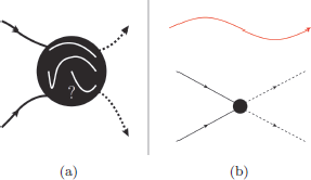
Since the hierarchy is so huge, being of order 10³², making boson light must be true when higher-order terms in quantum field theory are taken into account. Higher-order effects can be calculated by considering all possible Feynman diagrams with the same physical effects. Here, supersymmetry helps. In Fig. 6, we draw an idea on Feynman diagrams. In the discussion on the neutrino oscillation earlier, we commented that a relevant wave length is important. The wave length specifies the scale below which we do not question what really happens. In Fig. 6(a), the details inside the black ball are not recorded experimentally; look for the outside hints as far as the external observables are the same (two solid lines plus two dashed lines outside the ball). In Fig. 6(b), we show that the detailed structure cannot be seen with a large wavelength probe shown as a red curve, but quantum field theory provides a method to calculate in detail what is happening inside even though one cannot detect the inside phenomena.

Figure 6: Some ideas on Feynman diagrams. (a) Scattering by two solid line particles into two dashed line particles. (b) If the momenta are small corresponding to large wave length (in red), the scattering does not see the detail interior of a particle.

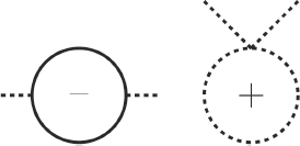
In the hierarchy problem, the Higgs boson mass is in question. Let us denote the Higgs boson mass in Fig. 7 with two outside dashed lines. Here, we showed what is happening for the Higgs boson mass at the one-loop level when the N = 1 supersymmetry is effective. When a fermion loop (the solid circle) contributes to the Higgs boson mass, its contribution is negative just because of the fermionic property of the antisymmetric contribution in Fig. 5 of Chapter 5. On the contrary, if a bosonic loop (the dashed circle) contributes to the Higgs boson mass, its contribution is positive because of the bosonic property of the symmetric contribution in Fig. 5 of Chapter 5. With the N = 1 supersymmetry, the magnitudes of these contributions are exactly the same. This means that the square of the coupling to the fermion is exactly the same as the boson coupling in the figure on the right-hand side of Fig. 7. The N = 1 supersymmetry provides a rationale for this equality. This is the supersymmetry argument to leave the Higgs boson massless at the Planck scale. The basic idea was assigning chirality to the Higgs boson.

Figure 7: Details contributing to the mass of the Higgs boson with N = 1 supersymmetry.

The next problem is how to generate the scale 246-GeV VEV of the Higgs doublet in the above supersymmetrised version. Here, one needs help from the gravitational interaction. Gravity extended with supersymmetry is called supergravity. Newton’s constant for gravity G_Newton is 6.67 × 10⁻¹¹ N · m²/kg² in the MKS units. Particle physicists often use the natural unit, which is called the Planck mass, M_P = 2.43 × 10¹⁸ GeV. So, gravitational interaction for energies of light particle introduces a ratio (Energy)/M_P. In this case, if we have some energy at the so-called intermediate scale, say at 5 × 10¹⁰ GeV, then the gravitational interaction induces a scale (5 × 10¹⁰ GeV)²/2.43 × 10¹⁸ GeV which is roughly 1,000 GeV. This can be used for breaking the electroweak symmetry. This road has been extensively pursued as a supersymmetric extension of the SM by many physicists. For the source of the intermediate scale, a mimic of the quark condensation for the chiral symmetry breaking in QCD has been adopted. It is the condensation of the supersymmetric partner of another strong force, which is usually called a confining gauge group in the hidden sector. Here, “hidden” means that this additional confining force does not interact with the SM particles. But, as of 2019, any expected supersymmetry partner of the SM particles listed in Fig. 5 has not been found at the highest energy accelerator LHC of CERN. “Now is the winter of our discontent,” lamented Shakespeare.

Fundamental particles so far explained are point-like particles with the observable sizes given by the (Compton) wavelengths. Can the fundamental particles have shapes as Plato’s solids of Fig. 4 of Chapter 1? Maybe strings. Strings were initially studied as the binding force of strongly interacting quarks under the name “dual resonance models” for which the first author reviewed in 1974 the work during 1968–1974,¹⁰ which went out of print in 1979, but was reprinted in 1986 by the World Scientific Publishing Company¹¹ and promptly sold three times as many copies as the original because of the new interest in superstrings.

With the discovery of the asymptotic freedom, however, QCD was accepted as the correct strong interaction dynamics and, at least for the strong interactions, dual resonance models were forgotten.

Meanwhile, it was known that the allowed extended shapes can be only strings in 10-dimensional space–time. There is one more condition: Strings in 10 dimensions should obey supersymmetry. In 1972, 10-dimensional superstrings were noted by Pierre Ramond (1943–), André Neveu (1946–), and John Schwarz (1941–). In 1974, Joël Scherk (1946–1980) and Schwarz advocated superstring theory for the source of gravity since string theory contained a massless spin-2 particle. This structure superstring must look like a point particle at the wavelengths employed in terrestrial experiments. Thus, super-string theories in 10 dimensions might be a possible extension of the SM at length scales shorter than the electroweak scale 10⁻¹⁶ cm. Ten years later in 1984, the real development of superstring theory bloomed when all the consistencies of 10-dimensional superstrings were proven, especially in the so-called heterotic string with the gauge group This group immediately attracted a great deal of attention because branching of E₈ leads to a spinor representation in the GUT group SO(10) and the second can be associated with the hidden sector needed for supersymmetry breaking. The spinor representation of SO(10) is signalling a chiral representation as commented before in relation to GUTs.

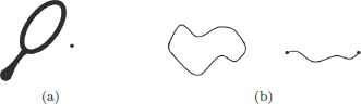
Figure 8: An extended object string: (a) a closed loop and (b) an open string.

The first obvious question one can ask is, “How large can a string be?” A natural answer will be its size is somewhat larger than the Planck length, probably around 10^{−31 to −32} cm. Then, if we look at the point-like particle with a lens of magnifying power 10¹⁶, as depicted in Fig. 8(a), it may look like Fig. 8(b). The heterotic string contains only closed strings whose dimensions are supposedly less than 10⁻³⁰ cm and there are string theories including open strings. Note that the Higgs boson Compton wavelength is about 10⁻¹⁵ cm. Another extreme case is to just allow the string length as large as possible but within the experimental limits from the search for long-range forces via the Cavendish-type experiments. Nima Arkani-Hamed (1972–), Gia Dvali (1964–), and Savas Dimpopoulos (1952–) initiated this kind of large-scale string theories of size 1 mm.

But, the above superstring is given in 10 space–time dimensions. We, living in the four space–time dimensions, must obtain a proper way of obtaining the SM from the 10-dimensional heterotic string. The process is called compactification, hiding six dimensions in 10 looking like internal dimensions to us. Work on the internal six dimensions suggested that they be of the Calabi–Yau shape, as initiated in 1985.

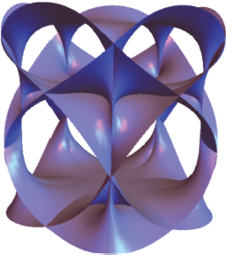
The idea of compactification is most easily understood by compactifying two real dimensions to one real dimension. Consider a sheet of A4 print paper which is a two-dimensional sheet. Then, roll it into a cigar shape. Making the radius of the cigar smaller, it behaves like a thick line becoming a thinner line. Effectively, we obtain one dimension if the wavelength of a probing eye is much larger than the cigar radius. A figure without the imaginery parts of the three complex Calabi–Yau is shown in Fig. 9. Generalising this idea of compactifying six dimensions, we obtain a four-dimensional theory. It must be supersymmetric since we started from superstring. So, if string is the mother of all fundamental particles, then supersymmetry must show up at some level, but we must wait.

Figure 9: A Calabi–Yau space.

It is hoped that the SM is obtained from some ultraviolet completed theory. For a consistent framework including gravity, therefore, derivation of the SM has been tried in the last three decades, including by the second author, from string theory because only string theory advocates calculable gravitational interactions. To the modern atomists, this attempt is not enough. The compactification should give all the parameters of the SM correctly. Even though some specific routes to the SM in the compactification are assumed, it belongs to a kind of God’s design since a definite route to the SM is taken.

Einstein’s gravity is said to be “metric” theory, which means that the equation for the metric tensor g_μν is Einstein’s gravity. In quantum mechanics, the action defined by the unit of the Planck constant ℏ is the key to understand how important the quantum effects are. The action is an integration of lagrangian (mentioned in the end of Chapter 4), L(t) = (kineticenergy)–(potential energy), with respect to time. More symmetrically, one defines L(t) as the space integral (∫ d³x) of the lagrangian L(x) at the space–time point x. Thus, the action is the space–time integral of the lagrangian (∫ d⁴xL). Einstein and David Hilbert (1862 AD–1943 AD) noted that the space–time integral of L multiplied with the squareroot of the determinant of g_μν gives Einstein’s gravity equation. In addition, if L contains a constant, it gives Einstein’s cosmological constant (CC), which Einstein introduced after a year of his first theory on the metric theory of gravity of 1916. If the gravitational interaction is given at such a small scale as 10⁻³³ cm, the first guess on the cosmological constant is (10⁺³³)⁴ cm⁻⁴, but the observed value is 10⁻¹²⁰ times smaller than that. This is the most severe problem, the cosmological constant problem, among hierarchies on the ratios appearing in physical theories. In compactifications, the CC is also calculated.

In 1998, astrophysical experiments confirmed that the universe is accelerating, with the CC of the order (0.001 eV)⁴. The above constant (10⁺³³)⁴ cm⁻⁴ is about 10⁺¹²⁰ times larger than this value. The number of compactified string models with the CC of this order to be present was estimated as 10⁵⁰⁰ by Michael Douglas (1961–). There are so many vacua, but there are some vacua with the CC less than (0.001 eV)⁴, which led to the idea of landscape scenario. String compactification allows, as far as the CC is concerned, some universe where our universe might have evolved with such a long history. All the others not belonging to this range of CC are ruled out because they have not lived this long history and humans could not have evolved. This landscape scenario belongs to the anthropic principle which was pointed out by Steve Weinberg and hence belongs to the evolution paradigm.

If quarks were not known, we could not complete the picture of 45 chiral fields in Fig. 5. This was the first moment of peeling the supposed atoms after Mendeleev found nuclei. Now, we turn to the story of how quarks in the universe were revealed to us humans.

__________________

¹J. Polkinghorne, Rochester Roundabout (R. H. Freeman and Company, New York, 1989), and Inspires C56-04-03, Proceedings of 6th ICHEP, Rochester, New York, USA, April 3–7, 1956.

²R. Leighton and E. Hutchings (editors) Surely You’re Joking, Mr. Feynman!: Adventures of a Curious Character (W W Norton, New York, 1985), ISBN 0-393-01921-7.

³T. W. B. Kibble, The Goldstone theorem, in Particles and Fields, Proc. of “International Conference on Particles and Fields, Rochester, N.Y., U. S. A., August 28–September 1, 1967, eds. G. S. Guralnik, C. R. Hagen and V. S. Mathur (Interscience, New York, NY, 1968), pp. 277–295.

⁴McCarthyism was the practice, during the cold war time of the early 1950s, of making accusations of subversion or treason without proper regard for evidence.

⁵J. C. Rigden, Rabi, Scientist and Citizen (Sloan Foundation Series, Basic Books, New York, 1987), ISBN 0-465-06792-1, OCLC 14931559.

⁶The word “flavour” is used for distinguishing different particles which however have the same electroweak interactions, i.e., interactions mediated by photon, Z and W^± in Fig. 5. On the Contrary, “colour” is used for defining strong interaction.

⁷If we consider loop effects, there are violation of P in gluon interactions, which lead to the so-called strong CP problem.

⁸The Planck mass is basically the inverse of the squarerooted Newton’s constant.

⁹R. Leighton and E. Hutchings (eds) Surely You’re Joking, Mr. Feynman!: Adsventures of a Curious Character (W W Norton, New York, 1985), ISBN 0-393-01921-7.

¹⁰P. H. Frampton, Dual Resonance Models (W. A. Benjamin, Reading, MA, 1974).

¹¹P. H. Frampton, Dual Resonance Models and Superstrings (World Scientific Publishing Co., Singapore, 1986).