Chapter 7

Order from Chaos

Before discussing mesons and baryons through which the systematisation of the hadrons in the 1960s is derived, we need to describe two transformative papers published, respectively, in 1954 and 1956, both involving Frank (Chen Ning) Yang (1922–). The second paper was briefly discussed in Chapter 6 and will be discussed further at the end of this chapter.

The first paper, with Robert Mills (1927–1999), provided a crucial generalisation of quantum electrodynamics (QED) which had already been established as a completely satisfactory theory of electrons and photons, agreeing with experiment to unprecedented accuracy. Today, the magnetic moment of the muon calculated from QED agrees with experiment to an astonishing one part in 1 trillion, the most accurate theory ever discovered.

The range of the electromagnetic force is practically infinite. If the wavelength is long enough, as in most cases (red colour in Fig. 6(b) of Chapter 6), one wavelength sweeps the whole region of the bullet in Fig. 6(b) of Chapter 6. There are two more fundamental forces which are effectively short-range forces compared to the electromagnetic force. Beyond electrodynamics, leptons and hadrons experience these short-range interactions which are strong and weak interactions. In the nucleus, these strong and weak forces are working only inside nuclei, i.e. in the black bullet in Fig. 6(b) if the bullet is identified as a nucleus. For the leptons, the strong force does not apply and the range of the weak force is similar to that in hadrons. This is a reason that weak force is sometimes called “weak nuclear force”. The story of weak force or weak interactions is the topic of Chapter 8.

The strong interactions hold together the atomic nucleus, overriding the electric repulsion between the positively charged protons. Since the strong force is restricted to the inside of the nucleus, it is a very short-range force. The reason it is short range (quark confinement) is completely different from that of the weak force. Now, the question is, “How can QED be generalised to accommodate this strong force?”

The key symmetry which underlies the success and uniqueness of QED is local gauge invariance. The force mediator in QED is the photon: gauge boson accompanied with the gauge principle. Pions were supposed to be the mediators for the strong force holding the atomic nuclei together, but they are not particles implied by some gauge principle. Before introducing the U(1) gauge principle for the photon, one considers the conservation of electromagnetic charge.

The charge conservation in quantum mechanics is the phase symmetry discussed in Chapter 5: Ψ → e^ieθΨ (e is the charge of electron) such that the observable probability Ψ^∗Ψ is invariant under this phase transformation. Invariance under this phase transformation is called “global” U(1) symmetry. It is “global” because θ is the same for any space–time points in the universe. QED involves making the phase depend on position x: Ψ → e^iqθ(x)Ψ, where q is the electric charge and parameter θ(x) (or sometimes the whole factor e^iqθ(x)) is the phase. Being the offspring of quantum mechanics, it is a unitary transformation. And, there is only one x-dependent parameter θ(x) by which we call it U(1) gauge theory, where we have interchangeable words (gauge) = (local). In QM dealing with electrons, the charge was the electromagnetic charge q = −e.

In Fig. 1(a), we show a global rotation. “Global” means that the same number is taken over all space. If we consider an electron orbiting around a proton (to this kind of electron, the atom is its whole universe), the electron wave function is depicted as the cloud in Fig. 1(a), which can be denoted as Ψ(x). The phase symmetry mentioned above is that rotation e^ieθ is the same at any point x. For Ne charge, then how can one calculate the global number? We enclose the source by a large closing bag, most conveniently a surface of a large sphere, the Gaussian surface, denoted as a yellow sphere in Fig. 1(a). Then, count all charges in this Gaussian surface. This is the way to count the global charges.¹ The phase rotation is for the whole wave function inside this yellow surface, Ψ → e^{iNe θ}Ψ.

Figure 1: U(1)’s: (a) A global rotation. (b) Gauge fields (E) from a charge q, where the red dashline depicts a Gaussian surface enclosing the charge. (c) Collecting E field lines of (b) into one direction. Here, the dashed circle is going around the collected flux lines of field.

For a U(1) “gauge” or “local” symmetry, the differences in the space–time points are usually denoted as a Taylor expansion, which in the continuum limit involves an expansion by denoted conveniently as ∂_μ. If the angle θ depends on x, i.e. θ(x), the difference in the nearby points involves ∂_μΨ(x). Then, ∂_μ(e^iNeθΨ) has to take account of acting ∂_μ on e^iNeθ(x). To make this effect unnoticeable, one must have a field compensating this derivative. It is called the gauge field A_μ, having the space–time index as ∂_μ. The photon in QED is introduced in this way.

In QED, how do we calculate the charge inside the Gaussian surface? Since θ(x) depends on x, we cannot calculate as done in Fig. 1(a). But, in the Gaussian surface, there are electric field lines going out from a positive charge as shown in Fig. 1(b). At each point on the Gaussian surface, we know the electric field E and we sum up the E field flux over the whole closure of the Gaussian surface. That sum is proportional to the total electric charge inside the Gaussian surface. If the surface is not closed, one cannot be sure that one measured the charge correctly. For example, one small hole can take out a significant portion of the flux, as shown in Fig. 1(c).

To render the short-range forces of strong and weak nuclear interactions as local ones, it is better to start with global symmetries as done above for U(1). Strong forces are mediated at the 100 MeV scale by three pions and hence U(1) is not a candidate for strong force. The weak nuclear force is effectively described by charged currents, which can carry positive or negative charge. Here again, therefore, U(1) is not suitable for the weak nuclear force.

In 1932, right after the discovery of neutrons, looking at the two particles, proton p and neutron n in the same way, Werner Heisenberg discovered a useful approximate symmetry. This is due to the fact that there is a very small mass difference 1.3 MeV between neutron n and proton p with their respective masses 939.6 MeV and 938.3 MeV. This was first measured by Chadwick and Goldhaber in 1933. So, the neutron–proton mass difference is just 0.15% of their average mass and hence Heisenberg considered them as the same in a first approximation. In this case, protons and neutrons behave in the same way as far as strong interaction is concerned, which is represented by the isospin group SU(2). The fundamental representation of SU(2) is two-dimensional, being proton and neutron, which is called a doublet. The doublet can be grouped as (p, n). The generalisation of this, looking at N particles in the same way, is SU(N), and its fundamental representation is then N-plet, (ψ₁, ψ₂, . . . , ψ_N).

The unitary transformation is the rule of transformation in quantum mechanics. For an N-plet, the transformation is done by the matrix multiplication where i, j, k, l vary from 1 to N. The number in the set ij in the exponent with the unitarity condition being N² for U(N), but proper counting for SU(N) is to subtract 1 from that (technically an SU(N)-transformation determinant is 1, adding S for special unitary group); thus, the allowed number of parameters θ_ij in SU(N) is (N² − 1).

As we generalised a global U(1) to a local U(1) before, now it looks like a simple matter to generalise a global SU(N) to a local SU(N). The idea of Yang and Mills was to consider this kind of more general phase transformation such that parameters θ_ij(x) are consistently introduced when they are made x dependent: in which g is a gauge coupling constant and M is a square N × N matrix. These N × N matrices generally do not commute and satisfy a non-trivial non-commutative algebra. The lagrangian for such a theory, called a Yang–Mills theory or a non-abelian gauge theory, generalises the QED lagrangian by introducing covariant derivatives to replace normal derivatives and a generalisation of the usual kinetic energy term, using the covariant derivatives. It was generally realised that the Yang–Mills idea was very likely to be a key ingredient in a correct theory, although it was several years before the appropriate application was identified. Remarkably, this Yang and Mills paper was never recognised by a Nobel Prize but did lead to at least 20 future Nobel Prizes.

The covariant derivative of the Yang–Mills theory needs a profound ingredient that includes a nonlinear term in the covariant derivative of the SU(N) gauge fields. This nonlinear term is the source for the asymptotic freedom and instanton solutions.

By 1960, there was a quite chaotic situation with respect to the many hadrons, baryons, and mesons which had shown up in experiments. There was no rhyme or reason until a breakthrough by Murray Gell-Mann in 1961 who realised that isospin, for which the symmetry group is Heisenberg’s global SU(2), must be enlarged to a global SU(3) with the additional rank used to accommodate strangeness quantum number S, a quantum number introduced by Gell-Mann earlier in 1955, for a subset of the mesons and baryons which did not decay by strong interactions.

As explained in Fig. 1(a), any global quantum number of U(1) for a wave function, or in the whole universe, can be measured. This is just for one quantum number. Heisenberg’s SU(2) considers only one diagonal quantum number in SU(2) even though it is a non-abelian global group. The number of diagonalisable quantum numbers is called the rank of the group in consideration. Diagonalisable ones are said to be commuting, and form what is technically called the Cartan subalgebra with dimension equal to the rank of the original group. If non-diagonalisable matrices are included, it produces “non-commuting” algebra. So, a non-abelian gauge group has a non-commuting algebra: non-abelian means non-commuting and abelian means commuting. If we consider two quantum numbers, we should consider U(1) × U(1). These two U(1)’s commute. But, combining with Heisenberg’s SU(2), we consider a rank 2 group SU(2) × U(1)_S, where U(1)_S denotes the group of transformation with the strangeness quantum number S.

Gell-Mann’s legacy starts by making the whole group SU(2) × U(1)_S a simple group of rank 2 with isospin SU(2) and strangeness U(1)_S. Rank 2 simple groups are limited: four classical groups SU(3), SO(4), SO(5), and Sp(4), and one exceptional group G₂. SO(4), SO(5), and Sp(4) are very short of satisfying the accumulated hadron data. Gell-Mann found his eight-fold way in SU(3), and declared that the needed non-abelian rank 2 group is SU(3). Here, we note that the group, including Ben Lee, at the University of Pennsylvania pushed for G₂, but Nature chose the eight-fold way and hence SU(3). Here, we emphasise again that the non-abelian group SU(3) is a global group but not a gauge one. As will be discussed in Chapter 8, in the current understanding of continuous symmetries, spin-0 pseudoscalars can be light due to spontaneous symmetry breaking of the mother global symmetry. If it were a gauge symmetry, we do not talk about spin-0 pseudoscalars but spin-1 gauge bosons. Therefore, to interpret pseudoscalar mesons, the symmetry must be global. But, in the early 1960s, it was not clear to physicists.

In terms of this global SU(3), called flavour SU(3), the mesons fall into singlet and octet irreducible representations. Indeed, there is one octet of pseudoscalars including the π and K mesons, and a second octet of vectors including ρ and K^∗ mesons, as shown in Fig. 2. The baryons are in octets and decuplets of SU(3). All mesons and baryons in a given irreducible representation have a common spin and parity, denoted as J^P . Observation of this regularity by Gell-Mann was remarkable. It was the first since the periodicity of chemical elements was found by Dmitri Mendeleev in 1859. In Gell-Mann’s SU(3), it is more intuitive to draw pictures in the plane rather than presenting with tables. Because its rank is two, i.e. two diagonalisable quantum numbers, usually the x coordinate is used for the third component of isospin and the y coordinate is strangeness S. Shifting the strangeness by the baryon number, sometimes “hypercharge” Y ≡ (S + B) is instead used as the y coordinate. The baryon octet for is shown in Fig. 2(a), and meson octets for J_P = 0⁻ and J_P = 1⁻ are shown in Figs. 2(b) and 2(c) as black bullets.

Figure 2: The eight-fold way: (a) Baryons, (b) pseudoscalar mesons, and (c) vector mesons.

Figure 3: The decuplet

There are baryons which are shown in a decuplet of in Fig. 3. When the baryons were studied in 1962, both Gell-Mann and Susumu Okubo (1930–2015) found that one component was missing. It was Ω⁻ with Mass = 1, 680 MeV, and strangeness S = −3. In particular, Gell-Mann made a very specific prediction that Ω⁻ particle decays principally by the mode Ω⁻ → Λ⁰ + K⁻ and Ξ⁰ + π⁻.

In an experiment at BNL by Nicolas Samios (1932–) and collaborators, the Ω⁻ with all the predicted properties was discovered, sealing the fame of Gell-Mann and the validity of the SU(3) classification, which he called the “Eight-fold way”. Thus, a chaotic situation was brought to order as the first real triumph of particle theory.

The success of SU(3) flavour symmetry led to the consideration by Gell-Mann in 1964 of the fundamental representation of SU(3), which is a triplet out of which all the hadrons might be made. We noted earlier in Chapter 6 that the fundamental representation of SU(3) was also considered by Shoichi Sakata in 1957, but the octet of baryons cannot be made in this way. Taking three quarks (as Gell-Mann called the hadron constituents, based on James Joyce’s Finnegan’s Wake) u, d, s, then the proton is (uud), the neutron is (udd), and the Ω⁻ is (sss). George Zweig (1937–) independently considered the same constituents, but with the name Aces. At first, this was presented as merely a mathematical shorthand, but as time progressed to the late 1960s, it became clear that the the quarks are physical and real point-like constituents of hadrons.

Given that quarks are fermions, one can extend SU(3) together with spin to SU(6) global symmetry from which baryon octet and baryon decuplet are combined together. These constitute 56 entries (8 × 2 + 10 × 4) in a single representation and SU(6) tells “Aha, 56 is completely symmetric under exchange of quarks!” More explicitly, for Ω⁻ = (sss), if all spins of s are up (which is contained in 56), then exchange of any pair is symmetric. But, the quark s is assumed to be fermion and the spin–statistics theorem implied in Fig. 5(a) of Chapter 5 requires total antisymmetry. This was a big hurdle to the quark model and Oscar Greenberg introduced Parastatistics in addition to the established Fermi–Dirac and Bose–Einstein statistics. A solution came from Moo-Young Han (1934–2016) and Yoichiro Nambu (1921–2015) with another non-abelian group which must be SU(3) under the assumption that, as in the eight-fold way, three quarks make up baryons. But, despite introducing additional SU(3) symmetry, it failed in correctly predicting the electromagnetic charges of quarks. In fact, they intended to introduce integer charge quarks because there was no hint of Gell-Mann’s fractional quarks in the universe. The electromagnetic charge is in the electroweak part and hence for strong interactions it does not matter, and we credit them as the first physicists to have introduced the additional SU(3) degree for strong interactions consistently with the spin–statistics theorem. The correct electric charges agreeing with Gell-Mann’s original charge assignment was discovered by Gell-Mann with Harald Fritzsch (1943–) in 1972, and a Yang–Mills theory for strong interactions using this SU(3) was put forward. This is called quantum chromodynamics (QCD). This is a different SU(3) from the eight-fold way, and acts not on flavour but on a new quantum number named colour. Each quark flavour comes in three colours called red, green, and yellow. QCD is now universally accepted as the correct theory of strong interactions, at least at accessible energies.

So far, we have discussed the strong force and its role to confine quarks within nuclear size, and in consequence the regularities appearing in the resultant hadrons. There are three fundamental issues here. One is how the strong force sticks the quarks together, and the second is seeing them by short wavelength probes. Finally, as for propagation of electromagnetic waves which are solutions of the QED field equations, can there be meaningful solutions of QCD field equations?

Regarding the second issue, at the very-short-distance scales probed by the high energy (at that time) electron beam of (=Stanford Linear Accelerator Center SLAC), Democritus’ idea was revived in the quark-parton model where the elementary quarks become evident in deep inelastic scattering as suggested by James Bjorken (1934–). In an article with Emmanuel Paschos (1944–), Bjorken pointed out that if you wish to see what is within the proton, you shine intense light to it. The scaling behaviour observed in high-energy electron and neutrino scattering experiments on nuclear targets completely agrees with the quark-parton model with nucleus containing three valence quarks. This success was possible because QCD behaves as if it interacts weakly at small separations, a property called asymptotic freedom. Asymptotic freedom was found by Harvard physicist David Politzer (1949–), and Princeton physicists David Gross (1941–) and Frank Wilczek (1951–). In addition, there are sea quarks and gluons. So, inside the proton, three valence quarks (uud) and “sea” quarks and gluons jiggle around. The quarks and gluons are indeed real physical particles.

Regarding the first issue, the asymptotic freedom guarantees that the QCD coupling constant becomes very strong at low-energy scale (at long-distance separations), providing an explanation for quark confinement and chiral symmetry breaking, not yet proven rigorously. Quark confinement is a simple word for why quarks are permanently confined inside hadrons and cannot be produced singly. The number of parameters of transformation under colour SU(3) is 3² − 1 as mentioned earlier and there are eight gluons. Because QCD is not broken, we listed gluons in Fig. 5 of Chapter 6 as massless particles. As mentioned earlier, even if gluons are massless, the strong force is short range due to the quark confinement or more generally confinement of all coloured particles, both quarks and gluons.

Regarding the third issue, let us refer to Fig. 1(b). In three space dimensions, the surface of the sphere denoted as the dashed curve is a balloon enclosing the sphere. The balloon is called a two-dimensional sphere denoted as S₂. In four space–time dimensions, Fig. 1(b) is a world line. World lines denote particle trajectories, and Fig. 1(b) in the world line is a trajectory of a charged particle.

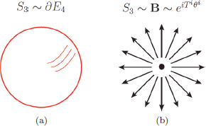
Can we consider a surface enclosing a four-dimensional sphere? For this purpose, consider a four-dimensional Euclidian space E₄. But, we cannot take a picture of a four-dimensional object. So, imagine Fig. 4(a) as just a four-dimensional sphere. Its surface is a three-dimensional sphere, which is denoted as S₃. A point (or a sphere in our case) in four dimensions is similar to hamiltonian or lagrangian because earlier we noted that action is ∫ d⁴xℒ.

Can we assign E or B fields on the surface S₃ of Fig. 4(a)? To have a perfect match on the position in S₃ of Fig. 4(a), the gauge fields must have the same geometrical property in the internal group space. Because S₃ is three-dimensional, we need three directions in the internal space. It is done with SU(2) internal space. We have repeatedly commented that the parameters in the unitary transformation are phases, which means that they are sitting on the surface of spheres of radius 1. SU(2) has three parameters and hence describes S₃ on the surface of unit radius. Thus, SU(2) gauge field strengths can sit on the S₃ of Fig. 4(a). These solutions, Fig. 4(b), are instanton solutions. “Instanton” is because they occur at one point (Fig. 4(a)) or instant in four-dimensional space–time. Since SU(2) is a subgroup of colour SU(3), the physics discussed with the instanton solution is applicable to QCD and to all non-abelian gauge groups. An explicit instanton solution was presented by USSR physicists Alexander Belavin (1942–), Alexander Polyakov (1945–), Albert Schwartz (1934–), and Yu. S. Tyupkin. This instanton solution was the beginning of finding out another parameter Θ in QCD, unknown before the discovery of the instanton solution.

Figure 4: Instanton.

In Fig. 4, the size of the ball appears necessarily. Since the nonlinear term of the gauge fields is the source of the instanton solution, this size is roughly the scale where this non-abelian gauge group becomes strong where the contribution is said to be O(1). If the instanton size is relatively smaller, then the effect of the instanton solution is exponentially suppressed compared to the O(1) contribution. For QCD instantons, this O(1) appears around several hundred MeV. If QCD becomes strong at a very-high-energy scale, due to the presence of many particles above the TeV scale, then one can consider correspondingly small scale instantons. But, there is no need to consider these extremely small instantons.

If non-zero Θ is present, QCD has a source of CP violation. QCD interactions do not violate the flavour symmetry, and hence the CP violation effects by strong interaction can be seen only by electric dipole moments. For the proton, its electric charge makes the dipole moment unobservably small even if it is present. So, the static property of neutron is the best test ground for the electric dipole moment. The current bound on the neutron electric dipole moment is about 10⁻²⁶ecm, restricting the bound on QCD’s |Θ| to about 10⁻¹² because the size of the neutron is about 10⁻¹⁴ cm. The QCD parameter |Θ|, intrinsically present, must be very small, which is a new type of hierarchy problem. In QCD, this is called the Strong CP Problem.

So far, we looked into the supposedly elementay particle proton and found out that there are more fundamental particles inside it: gluons and quarks. Without quarks, we are far away from filling out the particles of Fig. 5 of Chapter 6. This story invites us to make quarks and leptons composites of even more fundamental fermions under the name of urs and prions. But, such attempts have not been successful so far.

Gauge symmetries are the favoured symmetries in particle physics. One reason is depicted in Fig. 5, where the same angle is rotated on the Earth and on the Moon. The information of rotation on the Earth by angle θ to go to the Moon takes about 1.3 seconds at the speed of light and the simultaneous rotation at both places by the same angle θ is logically not allowed. But, if rotations depend on the position x, there is no need for θ (Moon) to be the same as θ (Earth). Thus, local symmetry is preferred by particle physicists.

In the standard model (SM) of particle physics, local symmetries are used for the elementary particle forces. Just counting the numbers, U(1) gauge symmetry is used for electromagnetism, SU(2) gauge symmetry is used for the weak interactions, and SU(3) gauge symmetry (which we called colour above) is used for strong interactions. Thus, the SM is gauge theory based on the gauge group SU(3) × SU(2) × U(1). The colour gauge symmetry SU(3)_colour is unbroken, but there is the important unsolved problem in SU(3)_colour: the confinement mechanism of colour. Now, we turn to the story of the electroweak gauge group SU(2) × U(1).

Figure 5: Global rotations.

Both of the Yang papers introduced at the beginning of this chapter played central roles in the discovery of the standard model. Parity violation is crucial because it necessitates using chiral fermions in the theory, which will be exploited in more detail in Chapter 8. This leads to constraints arising from the cancellations of quantum anomalies which would be automatically absent were parity to be respected.

Parity-symmetric nature, changing coordinate x to −x, was the God-given belief in the early days of quantum mechanics until 1956. In 1924, Otto Laporte (1902–1971) proposed that atomic wave functions are either symmetric or antisymmetric. Soon in 1927, Eugene Wigner (1902–1995) concluded that the Laporte rule was an aspect of parity-symmetric nature. As we know now, electrodynamics, the leading force working in the world of atoms, does conserve parity symmetry. Wolfgang Pauli was greatly influential in making particle physicists believe strongly in parity conservation. In atomic physics, it was very difficult to get any hint of parity violation. Even after the standard model was known, detection of parity violation from atomic physics was initially more difficult than in particle physics.

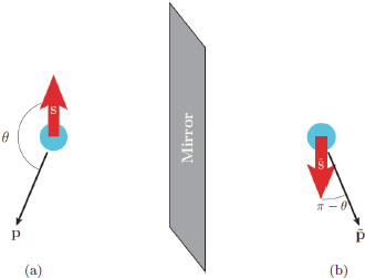
If parity is broken, it must be discovered from weak interactions, especially from decays of relatively long-lived particles. In Chapter 6, we already discussed this from the tau–theta puzzle. After the parity violation idea was mentioned in the ICHEP-6 Rochester conference, Tsung Dao Lee and Chen Ning Yang suggested that one can prove it from weak decay experiments such as Λ-decay and ⁶⁰Co-decay. If we take into account rotations, parity operation is identical to “mirror reflection”. In the mirror, left (L) and right (R) are changed. Why? Because you are standing up. So, devise an experiment to have a particle standing up. For this, spin direction is pretty good.

In Fig. 6, the essence of mirror reflection is depicted. Like a person standing up, a spin direction is given on the L-hand side. In the mirror, the spin direction is reversed because it is like the (orbital) angular momentum. The orbit is in the opposite direction in the mirror and the angular momentum direction is reversed. A particle moving with momentum direction p looks like in the mirror. The first confirmation of parity violation in weak decays came from this simple diagram performed by Madame Chien-Shiung Wu (1912–1997) at Columbia University. The nucleus was the radioactive isotope ⁶⁰Co with half-life 5.3 years. So, in nature it is not present. But, it can be manufactured artificially and has the magnetic moment which was aligned by the external magnetic field by Madame Wu. So, the spin direction is aligned to the upward direction as in Fig. 6(a). Suppose that the decay produces a particle with momentum p with the angle θ. The mirror reflection of this is shown in Fig. 6(b) going with angle π − θ with the spin direction. So, if nature is parity symmetric, we expect as many events in the southern hemisphere as in the northern hemisphere. What Madame Wu found was that there are more electrons coming in the southern hemisphere than in the northern hemisphere, and that parity is violated in the decay process. Nuclear beta decay is a weak process and it established a maximal parity violation in weak interactions.

Figure 6: A mirror reflection. This setup was used by Madame Wu for the decay of ⁶⁰Co.

__________________

1 The lepton and baryon numbers are also counted in this way.